A Dynamic CGE Model for Optimization in Business Analytics: Simulating the Impact of Investment Shocks

Abstract

This study formulates a mathematical dynamic Computable General Equilibrium (CGE) model within a rational expectations framework, adhering to neo-classical principles. It emphasizes the significant role of agents’ expectations in determining the broader economic trajectory over time. The model combines microeconomic and macroeconomic perspectives by merging the concept of intertemporal choice with savings behavior. Its mathematical foundations are derived and calibrated using data from a social accounting matrix to enhance its simulation capabilities. The paper presents a practical simulation investigating the economic implications of a strategic investment impact within an specific European region, Madrid as the case of study. Such demand shock affects sectors such as electronics, food, pharmaceuticals, and education. The study models the long-term effects of heightened investment and persistent demand-side shocks. The research demonstrates the CGE model’s ability to forecast economic shifts toward a new equilibrium after an investment shock, proving its utility for assessing the impacts of extensive environmental policies within a European context. The work’s originality lies in its detailed mathematical formulation, contributing to theoretical discourse and practical application in business analytics.

1. Introduction

The main objective of the article is to introduce a mathematically advanced, dynamic CGE model to address a wide range of challenges in resource planning and business analytics. This model seeks to optimize operations, identify market trends, and guide strategic decision-making, with a specific focus on simulating the impact of investment shocks on the economy. The originality of the study lies in its detailed mathematical formulation and innovative approach to simulating long-term economic impacts, making it an advanced and versatile analytical tool for predicting and evaluating economic dynamics in various scenarios.

The formulated dynamic Computable General Equilibrium (CGE) model, mathematically advanced to tackle a broad spectrum of resource planning and business challenges, is aimed at optimizing operations, identifying market trends, and guiding strategic decision-making. This model represents an innovative approach, augmenting traditional static CGE models with dynamic features, allowing for the simulation of long-term economic impacts and offering a detailed view of macroeconomic adjustments over time [1]. The study conducts a simulation to numerically analyze the economic effects of a strategic investment move, a crucial transition in the context of sustainable growth, particularly within Europe’s strategic framework [2,3].

At the core of this research is the mathematical construction of the CGE model, which embodies the microeconomic and macroeconomic foundations of intertemporal choice and savings. The model is grounded in a full, rational expectations, forward-looking neo-classical framework, exceeding the limitations of traditional recursive decision-making models. This forward-looking approach is key to the model’s utility in business analytics and long-term economic optimization, providing insights crucial for both regional and national policy-making.

The literature review emphasizes the importance of dynamic response modeling in capturing the complex economic effects of strategic shifts in environmental policies. Esteemed studies, such as those found in [1] and later published in [4,5,6], have paved the way for the application of CGE models to a variety of economic analyses.

A bibliometric study [7] analyzed 97 publications employing CGE (Computable General Equilibrium) models to examine climate change adaptation. This review highlights the flexibility of CGE models in depicting both sectoral and regional impacts, along with their advanced ability to track the temporal evolution of critical economic variables. In comparison to traditional CGE models, the study referenced in [8] provides a more detailed representation of energy and carbon emissions. It integrates environmental costs into the model more scientifically and examines the embodied carbon emissions in trade, offering innovative counterfactual analysis approaches. Furthermore, this paper discusses methods for extending and adjusting the model, enabling a wide range of modelers to develop a CGE model tailored to various requirements. All these works have demonstrated the models’ versatility in reflecting sectoral and regional impacts and their advanced capabilities in mapping the temporal progression of key economic variables.

Building on the comprehensive insights provided by these bibliometric studies, which establish the versatility and advanced capabilities of the CGE models, our paper takes a deeper dive into the mathematical foundations of the CGE model. We focus on its rigorous derivation and calibration using data from a social accounting matrix, ensuring the model’s accuracy in simulations and optimizing its application in business analytics and policy evaluation. This approach aims to furnish a robust analytical tool for exploring the economic consequences of strategical investment impacts, underscoring the necessity of such investments for fostering innovative, competitive, and sustainable growth.

Emphasizing the importance of such analytical tools in practical scenarios, the study then shifts its focus to the real-world application of these models. Specifically, it examines the economy of Madrid, Spain, assessing the impact of the strategic investment shift across various key sectors. This involves a detailed exploration of the sequence of economic adjustments following the strategic change, leading to a new equilibrium. The Community of Madrid refers to one of the 17 autonomous communities of Spain, which includes the city of Madrid and its surrounding metropolitan and rural areas. The paper’s concluding section will delve into the simulation’s effects on macroeconomic aggregates, spotlighting the key findings and their implications for future policy and economic strategy.

2. Literature Review

2.1. The Evolutionary Path of Applied General Equilibrium Models (AGEMs)

Tracing back to the mid-20th century, the field of economic modeling experienced a paradigm shift with the introduction of linear and nonlinear planning models. Pioneers such as Kantarovich and Koopmans [9,10] played a crucial role in this transition, moving beyond traditional input–output analysis to embrace optimization methods. This period marked the beginning of what would later evolve into applied general equilibrium models (AGEMs). The first model that garnered widespread recognition as an AGEM was introduced by Johansen in 1960 [11]. This era was further characterized by methodological innovations and a surge in practical applications, notably influenced by Scarf and Hansen in the early 1970s [12]. The AGEMs’ incorporation into mainstream economic research was significantly propelled by Shoven and Whalley [13], who expanded the Arrow–Debreu model to integrate aspects like government activities and international trade, previously unexplored in this context. Throughout the 70s and 80s, these models found extensive application in diverse fields such as trade analysis, fiscal policies, tax reforms, development strategies, and income distribution in developing countries. Notable studies conducted in nations like Korea and Brazil paved the way for this expansion. AGEMs also demonstrated their utility as tools for environmental policy simulation, particularly in researching the dual benefits of emission reduction and welfare and employment enhancement, with a focus on CO₂ emissions and energy savings [14].

In Spain, the introduction of AGEMs was marked by their use in analyzing the economic effects of the implementation of Value-Added Tax following the country’s accession to the European Economic Community in 1986 [15]. This initial application paved the way for broader usage in various economic policy analyses, including taxation, economic integration, immigration, energy, and more.

2.2. Static versus Dynamic AGEMs: A Comparative Overview

The inception of AGEMs brought forth static models, which provided a snapshot of the economic state at a particular moment, ignoring temporal changes or adjustments. These models were particularly beneficial for short-term economic policy analysis, offering insights into the immediate interactions between different sectors and agents. A noteworthy example of this application was the use of general equilibrium models for development policy, which highlighted the effects of changes in fiscal policy on income distribution during a specific year, without considering future economic trajectories [16] Another study presented a detailed framework for a static CGE model, demonstrating its utility in contemporary economic and policy analysis [17].

In contrast, dynamic AGEMs offer a broader, long-term perspective by capturing the intertemporal effects of policies and economic decisions. The economic growth models by Solow (1956) and Romer (1986) [18,19] exemplify this approach, explaining how economies evolve over time by incorporating factors like capital accumulation and technological advancement. These dynamic models provide a richer, more detailed view of economic processes, enabling researchers and policymakers to not only understand current impacts but also to forecast future effects of present decisions [20,21].

2.3. Dynamic AGEMs as Tools for the Optimization in Strategic Decision-Making

Dynamic AGEMs have proven to be valuable in optimizing strategic decision-making, especially in modeling the long-term economic implications of various policies within dynamic economic environments. For instance, a dynamic AGE model was utilized to assess the economic implications of photovoltaic (PV) energy generation investment and financing in Cameroon [22]. The model facilitated the simulation of different policy scenarios and their economic impacts, demonstrating how staggered increases in PV investment could accelerate industry development while minimizing economic growth impact. Further, dynamic trust mechanisms in financial inclusion markets were analyzed using a CGE model to achieve equilibrium in the rural financial sector, ensuring stable development [23]. These models have been applied at the country level for estimating reactions to technological changes, policy shifts, or external shocks like climate risks, global price changes, and recessions. Recent advancements in CGE models have been bolstered by improved micro-level data and the integration of macro–micro simulation modeling approaches, allowing for more detailed analysis of development policy impacts on household-level indicators such as poverty, employment, and diet quality [24]. Shibusawa [25] developed a dynamic multi-regional CGE model incorporating transportation networks to analyze the equilibrium and optimization of centralized and decentralized economies. This model addressed a social optimization problem, maximizing social welfare while adhering to intertemporal market constraints. Diao’s study on fiscal debt management in the Turkish economy highlighted the distortionary consequences and welfare implications of varying tax strategies [26]. Another study combined regional dynamic CGE modeling with optimal control to explore the influence of local government taxation and expenditure on regional growth, analyzing three policy regimes in terms of objective function gains, income inequality impacts, and model parameterization sensitivity [27].

2.4. AGEMs in Public and Private Sector Decision-Making

AGEMs have demonstrated their versatility and utility across both the public and private sectors. In the public realm, they provide critical insights into the impacts of policies like taxation or regulatory changes, and how these might influence different economic sectors. For instance, a study estimated the potential impact of COVID-19 on the United Kingdom’s economy, including the direct disease effects, preventive public actions, and associated policies [28]. This analysis can guide more effective health and economic policy formulation during a pandemic. In the private sector, AGEMs enable companies to predict and adapt to market or policy changes. They can be used to adjust business strategies in response to economic conditions such as demand fluctuations or operational restrictions.

In another study, the role of the production supply chain in climate policy choice was investigated, constructing an environmental dynamic stochastic general equilibrium (E-DSGE) model featuring multiple production stages and varying types of productivity shocks [29]. For the public sector, this provides a basis for understanding how different climate policies might impact supply chains and the overall economy. In the private sector, companies can use this information to anticipate the effects of climate policies on their operations and supply chains, enabling more informed production and logistics decisions. Continuing with more examples, another study examined the environmental and welfare impacts of pre-announced carbon policies using an E-DSGE model. It was found that pre-announcing a rise in the carbon tax rate could reduce CO₂ emissions but would also decrease output and investment during the interim period [30]. This information is vital for public sector decision-makers when formulating environmental policies, providing an understanding of the trade-offs between emission reductions and economic impacts. In the private sector, companies can use these insights to prepare for changes in environmental policy and plan their investments and operations more effectively, minimizing the negative impacts on their economic performance.

2.5. Dynamic AGEMs as Business Analytics Tools

Optimization tools like AGEMs, especially in their dynamic forms, have found a new role as business analytics tools. Business analytics, focusing on data use, statistical analysis, and mathematical models for informed decision-making, includes data collection, processing, and analysis to understand and analyze business performance. Within this framework, optimization tools are used to identify the best possible solutions or the most effective strategies against a set of options, constraints, and business objectives. Business analytics helps companies leverage the value of historical data by harnessing the power of statistical and mathematical models and advanced techniques such as artificial intelligence algorithms. As the field evolves, its applications continue to broaden, adapting to various functional departments within enterprises and extending to non-business areas [31]. These models, as optimization tools, integrate into the prescriptive aspect of business analytics, enabling businesses and organizations to simulate and understand how different variables and decisions interact within a complex economic system. They offer a holistic view of how different elements of an economic system interact, which is crucial for business analysis. They facilitate strategic decision-making by providing insights into the potential consequences of various actions and policies. Lastly, they allow organizations to adapt and plan based on changing and complex economic scenarios, which is essential in a dynamic and globalized business environment. In a recent study that conducted a literature review on the current concept of business analytics [31], the most used tools or techniques in this discipline were specified. However, equilibrium models are not among them; some of the techniques used in this area are specified, but the models of equilibrium are not.

This work not only enriches the theoretical understanding of dynamic Computable General Equilibrium (CGE) models within a framework of rational expectations but also fills a critical gap in the practical application of business analytics across a variety of strategic contexts. The originality of this study lies in its complex mathematical formulation and its innovative approach to simulating long-term economic impacts, which is crucial for a wide range of strategic decisions in different sectors. This model stands out as an advanced and versatile analytical tool, capable of predicting and evaluating economic dynamics in a variety of scenarios, including but not limited to changes in environmental policies. Its significant contribution to the theoretical and practical discourse in business analytics makes it a valuable resource for informed decision-making in both the public and private spheres, contributing importantly to strategic planning and analysis in an increasingly complex and dynamic global economic environment.

3. Materials and Methods

The evolution of economic models from input–output analysis to dynamic Computable General Equilibrium (CGE) models represents a significant advancement in the field of economic modeling, reflecting a progression toward greater complexity and realism.

Input–output analysis marked the beginning of this journey. It provided a mathematical framework for understanding the interdependencies between different economic sectors using linear equations. While this model offered insights into the structural characteristics of the economy, it was limited in scope, primarily capturing direct interdependencies among sectors and overlooking broader income-induced effects across markets.

Building on this, Linear General Equilibrium Models emerged, utilizing the social accounting matrix (SAM) framework. These models expanded the analytical scope to include all transactions of goods, services, and income among various agents and sectors, providing a more comprehensive view of economic flows. However, the linear nature of these models imposed constraints such as constant returns to scale and fixed relative prices, limiting their ability to reflect real-world economic complexities.

To address these limitations, applied general equilibrium models (AGEMs) were developed. AGE, with its non-linear mathematical structure, integrated more complex economic behaviors like optimization in competitive markets, substitution processes, and endogenous labor market dynamics. This model represented a significant leap in capturing the nuanced interactions and functions of various market sectors and economic institutions.

The dynamic CGE model represents the culmination of this evolution. It builds upon the foundations laid by the earlier models but surpasses their limitations by incorporating dynamic elements into the CGE framework. Utilizing the SAM as its database, the dynamic CGE model can simulate the evolution of an economy over time, factoring in changes in technology, demographics, and policy. This model’s ability to incorporate dynamic transitions and adjustments offers a more realistic and nuanced understanding of economic phenomena, representing the forefront of current economic modeling practices.

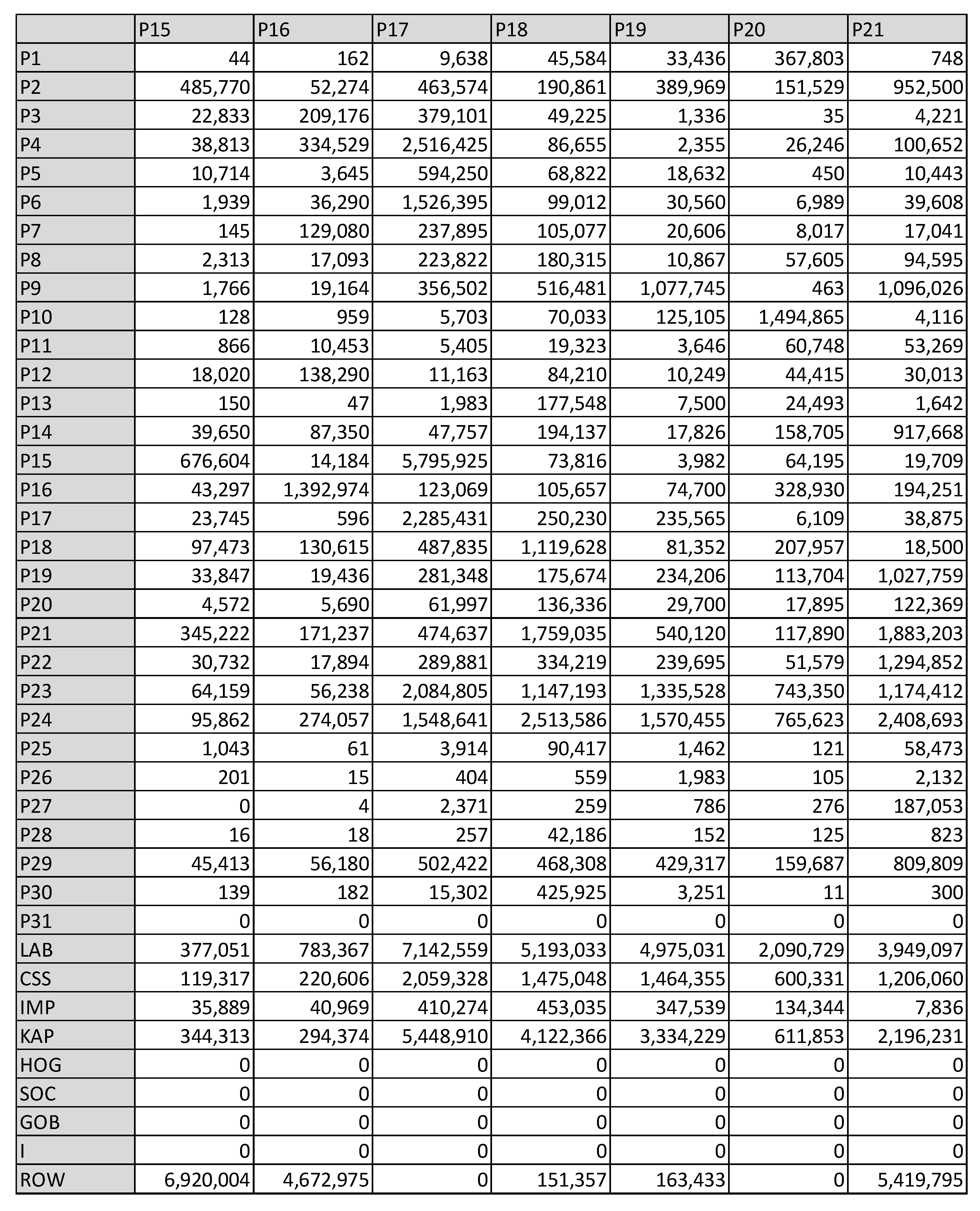
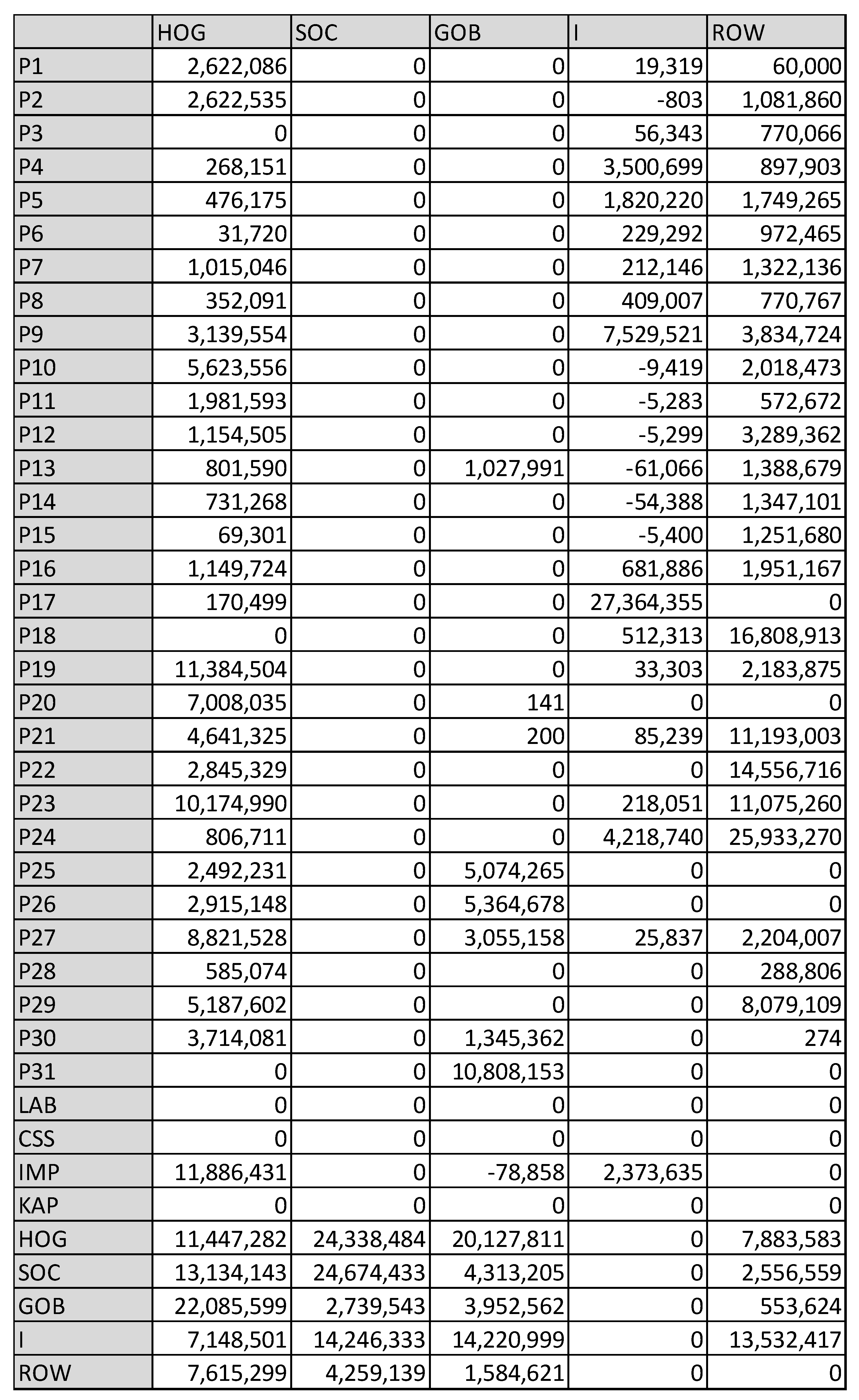
Upon estimating the social accounting matrix, a robust statistical framework is established. This framework not only facilitates the calculation of linear multipliers but also underpins the development of applied general equilibrium models. Specifically, the social accounting matrix for the Community of Madrid, as calculated for the year 2005, offers an appropriate database. This database is instrumental in simulating the mathematical model, effectively applying the formulated mathematical model to real-world scenarios.

The selection of the year 2005 for the social accounting matrix in this study was dictated by the availability of relevant data for the Madrid economy. Due to the absence of an official matrix, the 2005 matrix was constructed using the available macroeconomic data. The creation of such matrices is not straightforward and demands extensive research. Specifically for this model, the Madrid 2005 matrix was meticulously estimated, signifying a notable research endeavor. This process underscores the complexity and significance of accessing and utilizing databases in research. The primary objective of this specific exercise is to demonstrate that the mathematical model is functional and applicable, using an appropriate database. By choosing this particular set of data, the study acknowledges the ever-evolving nature of economies and prioritizes the model’s formulation over the mere assembly of a database, thus shedding light on the study’s core principles and inherent constraints.

The mathematical formulation of the mathematical program is encoded with a computational algorithm that will be solved using the GAMS^® software (39.1.1). The dynamic CGE includes, among its assumptions, optimizing behavior in competitive markets and allows for the incorporation of substitution processes, an endogenous labor market, price incentives, and shadow prices, as well as technological differences between various sectors.

The simulation of the impact on the economy, in this case the Community of Madrid, allows for the analysis of the transformation of its productive structure as a result of an investment shock in each of the selected sectors.

3.1. General Structure of a Computational Applied General Equilibrium Model

Throughout various existing works on the development of CGE models, we find a common methodology in their design. It is customary to build them in three successive stages, each characterized by common objectives and elements (Figure 1). These stages are:

(a)

Model formulation

(b)

Model calibration

(c)

Policy simulation in the model

Figure 1. Stages in the development of a CGE model. Source: own elaboration.

Figure 1. Stages in the development of a CGE model. Source: own elaboration.

Once the problem or economic analysis to be solved is determined, the main objective of the first stage will be the qualitative or theoretical presentation of the model. This will require specifying, among other aspects, the functioning of the markets, the behavior of the agents, and their classification. Additionally, this phase will conclude by determining the concept of general equilibrium used, along with the type of closure adopted.

-

Model Formulation: The first stage consists of the theoretical presentation of the model, specifying the functioning of the markets, the behavior of the agents, and their classification, and determining the concept of general equilibrium and the type of closure adopted.

-

Model Calibration: The second stage involves the numerical specification of the model to represent the economy studied over a specific period or several periods, using the accounting and statistical data collected in the social accounting matrix (SAM). This includes the initial resolution of the model to replicate the current economic equilibrium.

-

Policy Simulation: The last stage involves varying some exogenous variables and solving the model’s equations to obtain a new equilibrium, thus evaluating the effects of certain economic policies.

Foundations of the Dynamic CGE Model

It is based on the hypothesis of rational expectations of agents, including a detailed sectorial breakdown of the main markets, as well as capital and labor factors.

The common economic agents modeled include the productive sectors, consumers, the public sector, investment and savings, and the external sector.

-

Producers: Considered maximizing agents with long and short-term objectives. The formulation includes production functions with constant returns to scale and nested supply structures.

-

Consumers: Modeled as agents who maximize the present utility of their aggregated utility function over their expected lifetime, subject to a budget constraint.

-

Public Sector: Acts as an intermediary in certain economic flows, performing income tax redistribution and affecting the economic sphere of the Madrid region.

-

Investment and Savings: Focuses on the dynamics of investment as a component of final demand and savings as deferred consumption.

-

External Sector or the “Rest of the World”: Includes the interaction of the analyzed economy with foreign economies, generally employing the Armington assumption of imperfect substitution between national and imported products.

The formulation of the theoretical model is just the first step in the development of a CGE model since one of the objectives of these models is the empirical analysis of a specific real economy. Therefore, a second stage is necessary, consisting of the numerical specification of the model, in such a way that it represents the economy studied for a specific period or over several periods of time. Traditionally, this process is carried out through so-called model calibration using the available accounting and statistical data collected in the social accounting matrix (SAM).

The initial resolution of the model, by specifying it numerically (without varying any of the values of the exogenous variables), offers us an initial or reference equilibrium of the economy, replicating the current economic situation (for the analyzed period). This will enable the achievement of the second objective of a CGE model: the evaluation and analysis of the effects of certain economic policies.

To assess these effects, simulations will be performed in the model, varying some of the exogenous variables and subsequently solving the model’s equations to obtain a new equilibrium.

Here, we provide a detailed breakdown of each stage involved in constructing an applied general equilibrium model.

3.2. Mathematical Formulation of the Dynamic Applied General Equilibrium Model

To achieve the goal of constructing applied models that accurately represent the most significant economic sectors and capture the unique features of the economy under study, the researcher’s approach centers around two main axes:

-

The specification of the intervening agents and their assumed behavior.

-

The definition or concept of equilibrium used.

Building upon these foundational aspects, policy impact simulation has recently evolved due to modern prospective tools such as dynamic CGE models for macroeconomic analysis. The original model is the Ramsey (1928) model and is the one which allowed Solow [18] and Swan [32] to develop the methodological basis of later models. They depicted the assumptions and hypotheses that are to be incorporated into such models to capture and synthesize agents’ behavior.

The mathematical foundations of dynamic modeling are summarized in [33], so now we face the challenge of adapting and applying them to the wide range of situations that are given in real economies. Since modeling involves a certain degree of approximation to reality, these models are subject to continuous revision and updated. In the specific case of Madrid´s region, a social accounting matrix (SAM) referring to the year 2005 [34] was constructed so that it provides the framework linking together the economic behavior of the representative aggregate agents.

The following figure (Figure 2) can be observed for an overview of the problem statement and to summarize the analysis method applied in this work by means of the dynamic CGE model:

The present formulation of our dynamic CGE model is based on the rational expectations hypothesis of the agents; thus, the proposed architecture consists of a detailed sector breakdown where the main markets appear, as well as capital and labor.

The assumption of rational expectations in applied general equilibrium models is a crucial concept in modern economic theory. It refers to the hypothesis that agents within an economy—individuals, businesses, and other organizations—make decisions based on a rational outlook, the available information, and their past experiences. Here is a breakdown of how this assumption plays out in these models:

• Agents are presumed to make forecasts about future economic variables in a way that optimally utilizes all available information. This means their predictions are not systematically biased and are as accurate as the model and available information allow.
• Agents are assumed to consider all relevant and available information when forming their expectations about future economic conditions. This includes historical data, current economic indicators, and an understanding of economic policy and its potential impacts.
• In a general equilibrium model, rational expectations imply that agents’ predictions about economic variables are consistent with the model itself. Their expectations are formed in such a way that, on average, they will coincide with the model’s predictions.
• An important implication of rational expectations in these models is that economic policies will not have systematic and predictable effects if agents adjust their behavior in anticipation of these policies. For instance, if a government announces an inflation target, agents will anticipate this and adjust their behavior accordingly, which will be reflected in the equilibrium of the model.
• In dynamic general equilibrium models, rational expectations also play a key role in how economies adjust over time. Agents form expectations not just about current conditions but also about how the economy will evolve in the future, influencing their current decisions.

The assumption of rational expectations in applied general equilibrium models posits that all agents in an economy make informed, forward-looking decisions that are consistent with the model’s structure. This has significant implications for understanding how economies respond to policy changes and how equilibria are formed and adjusted over time.

• Justification of the Assumptions in the Model

The dynamic Computable General Equilibrium (CGE) model presented in this section is based on the hypothesis of the rational expectations of the economic agents. This hypothesis is a crucial concept in modern economic theory and assumes that agents make decisions based on a rational perspective, the available information, andtheir past experiences. It is highlighted that agents make forecasts about future economic variables by optimally utilizing all available information, implying that their predictions are not systematically biased and are as accurate as the model and information allow.

This formulation of the dynamic CGE model is important as it captures the anticipatory behavior of agents in the economy, allowing for a more realistic and detailed analysis of how economies respond to policy changes and how equilibria are formed and adjusted over time. However, the assumption of rational expectations also entails certain limitations, as it presupposes a high level of information processing and foresight by the agents, which may not always reflect decision-making in the real world. In addition, models based on rational expectations can be complex and demanding in computational terms.

The assumptions of the dynamic CGE model, although strict, are fundamental for its application and relevance in economic analysis. These assumptions allow the model to realistically simulate how economic agents, such as individuals, companies, and other organizations, make informed and anticipatory decisions that are consistent with the structure of the model.

These assumptions are key to understanding how economies respond to policy changes and how equilibria are adjusted over time. The incorporation of rational expectations ensures that the model not only simulates immediate reactions to policy changes but also takes into account how agents adjust their behavior in anticipation of these changes. This feature is crucial for analyzing the long-term impact of policies and investments, especially in the context of expectations and market dynamics.

Although disciplines such as behavioral economics and institutional economics may question some of these assumptions, arguing that agents do not always act fully rationally or are not informed, these criticisms do not invalidate the usefulness of the dynamic CGE model. Instead, they provide important context and highlight the need to interpret the model’s results within a broader framework that includes behavioral and institutional considerations. These additional considerations can enrich the analysis and offer a more nuanced perspective on economic impacts.

• The Agents

Outlined below are the key aspects and critical decisions that a researcher must consider in modeling the most common economic agents in any CGE model. These agents are categorized into:

(a)

Productive sectors

(b)

Consumers

(c)

The public sector

(d)

Investment and savings

(e)

The external sector

The model constructed here incorporates the conduct of these representative agents of the economy: 31 production sectors, a representative consumer of Madrid’s households, the owners of the production factors (capital and labor), the public sector (which collects taxes, provides public goods and services, and performs transfers), and finally the so-called aggregate rest of the world, which brings together the entire foreign sector as a single aggregate account.

A comprehensive description of the equations comprising the constructed model is provided below.

3.2.1. Producers

When modeling productive sectors, it is necessary to make adjustments not only to the number of productive branches but also ti the type of grouping or disaggregation that is most convenient for the analysis of the economy to be conducted. It should be considered that excessive disaggregation of the productive sector could complicate the interpretation of the results that the model will eventually provide.

Another assumption that must be established in the model is the functioning of the markets for produced goods, as this will determine the behavior of each of the producers. In relation to this assumption, there are two types of modeling in the literature: on the one hand, traditional and more orthodox models with the concept of Arrow–Debreu equilibrium that employ the assumption of perfect competition in all markets, and on the other, models that incorporate the existence of imperfect competition in some markets.

Models that incorporate imperfect competition show great diversity, making it difficult to present a common structure among them. This diversity is due to the multiple forms of competition (monopoly, collusion, oligopoly, etc.) and the variety of rivals’ reactions, represented using conjectural variations, Cournot/Bertrand models, etc. [35]. On the other hand, the geographical framework in which companies compete (integrated or segmented markets) is also relevant, as the demands and competition they face in each framework can vary. In this work, we have included only a description of the formulation of models with perfect competition. A detailed review of the different types of models with imperfect competition can be found in [36].

The next consideration to be made is to determine the functional form through which the combinations of factors and other inputs (intermediate consumption, imports, etc.) are related to determine the production technology function of the hypothetical homogeneous good manufactured by each of the productive branches represented in the model.

Under the assumption of perfect competition, it is usual for this productive technology to be described using production functions that have constant returns to scale, and the most commonly chosen forms are a Leontief or fixed coefficient, Cobb–Douglas type, CES (constant elasticity of substitution), LES (Linear Expenditure System), and Translog.

The choice of a specific form will normally depend on how the elasticities will be used in the model and on the availability of statistical data related to these elasticities, which allow their numerical specification in the calibration process.

Moreover, in the description of productive relationships, there is the possibility of incorporating nested structures of supply, thus defining different levels of combination of the inputs of the productive process. In most of the applied models existing in the literature, this is usually divided into three levels of nesting: at the first level, the composite good or added value is obtained by combining the productive factors (capital, labor, etc.). The domestic production function is the result of the second level of nesting through the combination of the composite good and intermediate inputs. Finally, at the third level, in the case of open economies, domestic products are combined with imported products to determine the total production function. This is illustrated in the diagram featured in Figure 3.

In the first level of nesting, we propose the total production equation of the goods offered by each sector in each period. We adopt the Armington assumption, commonly used in the literature on the subject in these cases, by which we define the total production as a composite good of the domestic production and imports, combining both inputs using a Cobb–Douglas function:

$$Q_{j(t)}={\beta }_j·X{D}_{j(t)}^{{\alpha }_j}·M_{j(t)}^{(1-{\alpha }_j)}$$

(1)

where ${\beta }_{j(t)}$ represents the efficiency coefficient of the total production function. The coefficients ${\alpha }_{j(t)}$ and $(1-{\alpha }_{j(t)})$ represent the technical coefficients of the domestic production and imports, respectively.

In the second level of nesting, the domestic or interior production function $X{D}_{j(t)}$, of each sector $j$ at each moment $t$ is obtained by combining intermediate consumption and value-added using a fixed coefficient transformation function, Leontief-type:

$$X{D}_{j(t)}=\underset{i=1\dots 31}{\mathit{min}}\left\{\frac{x_{ij(t)}}{a_{ij}};\frac{{\mathit{VA}}_{j(t)}}{v_j}\right\}$$

(2)

With $a_{ij}$ being the requirement of good $j$ to produce one unit of good $i$ and $v_j$ the value-added component per unit of production of sector $j$.

In the third level of nesting, we assume that each sector produces in perfect competition and with constant returns to scale, which is reflected in a value-added equation $V{A}_{j(t)}$, with Cobb–Douglas technology that combines the capital and labor factors:

$$V{A}_{j(t)}={\upsilon }_j{K}_{{}_{j(t)}}^{{\theta }_j}{L}_{{}_{j(t)}}^{(1-{\theta }_j)}$$

(3)

where $K_{j(t)}$ is the capital factor of sector $j$ in the period $t$, $L_{j(t)}$ the labor factor used by the sector $j$ in the period $t$, and ${\theta }_j$ and $(1-{\theta }_j)$ represent the technical coefficients of the production factors, capital and labor, respectively. The parameter ${\upsilon }_j$ is the efficiency coefficient of the added value that represents the technology with which the productive factors are combined at this third level of nesting.

We will consider producers to be maximizing agents with two types of objectives: an intertemporal long-term goal and, on the other hand, a set of intratemporal goals.

The last consideration refers to the behavior of firms, as rational behavior will facilitate the determination of the demanded quantities of factors and other inputs, as well as their corresponding prices. The rational behavior of the producers is assumed to be directed at maximizing their profits, subject to their technological constraints.

However, specifying production functions with constant returns to scale implies that no activity offers positive profits at market prices. Therefore, the necessary condition for profit maximization is that producers minimize their production costs, and solving these mathematical programs will provide the model’s equations for the demands of the productive factors and other inputs of the productive process.

Producers will be considered maximizing agents with two types of targets: an intertemporal long-term objective and, secondly, a set of intratemporal objectives solved as in any static CGE model of a certain period.

Under the dynamic approach, and in relation to every producer´s evolution of capital, we assume that the capital stock of each company at the beginning of each period $K_{j(t+1)}$ is equal to that in the previous period $K_{j(t)}$, underestimated by the depreciation plus the investment made $IN{V}_{j(t)}$ at the end the previous period, i.e.:

$$K_{j(t+1)}=(1-{\delta }_j)K_{j(t)}+IN{V}_{j(t)}$$

(4)

where ${\delta }_j$ is the rate of depreciation for the capital factor, whereas the capital stock for the first period is exogenously fixed.

If the representative producer behaves under rational forward-looking expectations, which involve no uncertainty or absence of money illusion, the producer uses in each period an amount of labor and capital inputs such that the firm value is maximized. As a result of this decision, the level of investment $IN{V}_{j(t)}$ is obtained, which makes the degree of capitalization of the company vary period after period.

Under this approach, we refer to the dividend payments made by the company, calling them $DI{V}_{j(t)}$, with the value of the production of the company proving to be $PV{A}_{j(t)}·V{A}_{j(t)}$ lowered by the cost of the labor factor, taking into account social security payments $P{L}_{j(t)}·L_{j(t)}·(1+taxcss)$ and minus the costs related to investment, $IN{V}_{j(t)}$ and ${\mathsf{\Phi }}_{j(t)}$.

Thus, we obtain the expression of dividend payments, which becomes:

$$\begin{array}{l}DI{V}_{j(t)}=PV{A}_{j(t)}·V{A}_{j(t)}-P{L}_{j(t)}·L_{j(t)}·(1+taxcss)-\\ -br·P{K}_{j(t)}·IN{V}_{j(t)}-PV{A}_{j(t)}·{\mathsf{\Phi }}_{j(t)}\end{array}$$

(5)

The last two terms refer to the aforementioned costs associated with investment in each period: the first one is associated with the part of the producer investment financed by the retained earnings, $br·P{K}_{j(t)}·IN{V}_{j(t)}$, and the second term, $PV{A}_{j(t)}·{\mathsf{\Phi }}_{j(t)}$, represents the adjustment costs associated with the new investments made by each firm in each period. The latter collect losses arising, for example, in the adjustment process after the implementation of a technological improvement in a company or any progress toward successful implementation, applicable to any other similar situation. The existence of such adjustment costs implies that companies lose part of their production in the investment process, so the desired capital stock is achieved over time gradually and not instantly, in an abrupt way.

In the context of this long-term vision of the producer, as the objective is to maximize the financial value of the company, labeled $V_j^0$, it is defined as the present value of the flow of future dividend payments by the company, proving to be its expression as follows:

$$V_j^0={\displaystyle \sum _{t=1}^{\infty }{\displaystyle \prod _{s=1}^t\left(\frac{1}{1+r_s}\right)·(DI{V}_{j(t)})}}, \forall t=1\dots \infty$$

(6)

The optimizing behavior of the producer implies achieving a balance in the financial value of the companies using different interest rates, $r_s$, for each period.

In this equation, $r_s$ is the interest rate at any time previous to year $t$, $V_{j(t)}$ is the market value of company $j$ at time $t$, $DI{V}_{j(t)}$ are the dividends paid by the company $j$ in the year $t$, and $V_{j(t+1)}^0$ is the market value of the company $j$ at time $t+1$. So, the market value of the company $j$ at time $t+1$ is given by the expression:

$$V_{j(t+1)}=V_{j(t+1)}^0+V_{j(t)}^N$$

(7)

where $V_{j(t)}^N$ is the new shares issued by the company $j$ at time $t$. These new shares are to be part of the investment, which is not financed with retained earnings, i.e.,:

$$V_{j(t)}^N=(1-br)·P{K}_{j(t)}·IN{V}_{j(t)}$$

(8)

Given that $br$ is the coefficient of the retained earnings by the company, $(1-br)$ will then be the partition coefficient to the shareholders of the company.

With this approach and substituting in Equation (6), which represents the expression of the dividend payments, we obtain the equation for the financial value of the company, which turns out to be the objective function in the optimization program of the company, subject to the constraints of added value (3) and capital (4).

$$\begin{array}{l}{V}_j^0={\displaystyle \sum _{t=1}^{\infty }{\displaystyle \prod _{s=1}^t\left(\frac{1}{1+r_s}\right)·\left[PV{A}_{j(t)}·V{A}_{j(t)}-P{L}_{j(t)}·L_{j(t)}·(1+taxcss)\right.}}-\\ \left.-br·P{K}_t·IN{V}_{j(t)}-PV{A}_{j(t)}·{\mathsf{\Phi }}_{j(t)}\right]\end{array}$$

(9)

Thus, we obtain the program for maximizing the value of the company, which the producer faces in the long term, formulated as follows:

$$P_j\left\{\begin{array}{c}Max V_j^0\\ s.t:K_{j(t+1)}=(1-{\delta }_j)K_{j\left(t\right)}+IN{V}_{j\left(t\right)}\end{array}\right. \forall j=1,\dots ,31.$$

(10)

where producers allocate their optimal investment strategies and use of factors, ${\left\{IN{V}_{j(t)},L_{j(t)},K_{j(t)},\dots \right\}}_{t=1\dots \infty }$, to maximize the present value of the company, taking into account the expected price of sale of production, the cost of investment, and the labor costs, ${\left\{PV{A}_{j(t)},P{K}_{j(t)},P{L}_{j(t)}\right\}}_{t=1\dots \infty }$, subject to the constraints on capital accumulation. Thus, solving the above equations, we obtain the model equations related to the intertemporal equilibrium values of the model variables.

Thus, by solving the previous program, we obtain the following equations of the model:

$$PV{A}_{j(t)}·{\mathsf{\Phi }}_{j(t)}^{\prime }+P{K}_t={\lambda }_{j(t+1)} t=1,\dots ,T-1$$

(11)

$$\begin{array}{l}\left[PV{A}_{j(t)}·{\alpha }_j·\frac{V{A}_{j(t)}}{K_{j(t)}}+PV{A}_{j(t)}·{\mathsf{\Phi }}_{j(t)}\right]+\\ +(1-{\delta }_j)·{\lambda }_{j(t+1)}-(1-r_t)·{\lambda }_{j(t)}=0 t=1,\dots ,T-1\end{array}$$

(12)

$$K_{j(t+1)}=(1-\delta )·K_{j(t)}+IN{V}_{j(t)} t=1,\dots ,T-1$$

(13)

$$L_{j(t)}=\frac{PV{A}_{j(t)}·V{A}_{j(t)}·(1-{\theta }_j)}{P{L}_{j(t)}·(1+taxcs{s}_j) } t=1,\dots ,T-1$$

(14)

A feature of the dynamic approach is the treatment of capital in the last period of the formulation, which we call the final period or year “T” [37], representing the model´s terminal period. Empirical models can only be solved for a finite number of periods, and a numerical solution cannot be obtained in a formulation which foresees an infinite number of periods. Thus, it is necessary to make some adjustments in order to approximate our infinite horizon model into a finite horizon one.

A specific formulation allowing capital stock to reach its steady-state level in the terminal period was therefore introduced. According to Lau et al. (1997), the level of post-terminal capital stock as a variable is incorporated, and a constraint on the growth rate of investment in the terminal period is added [37]. The advantage of using this constraint is that it imposes growth in accordance with the previous path; hence, the constraint on investment in the terminal period can be formulated:

$$IN{V}_{j(T)}=(g+\delta )·K_{j(T)}$$

(15)

$$PV{A}_{j(T)}·{\mathsf{\Phi }}_{j(T)}^{\prime }+P{K}_T={\lambda }_{j(T)}$$

(16)

$$r_T=\rho$$

(17)

This method assumes that the economy is in a steady state after simulation by the terminal period T; it is a method of approximating infinite-horizon choices, but it is solved over a finite horizon, following [38].

Producers’ Intratemporal Optimization

Producers, in addition to maximizing the long-term financial value of the company, maximize profits (or equivalently, minimize production costs, given that the production function exhibits constant returns to scale) in each time period at each of the last two nesting levels. The resolution of the following program for minimizing the production costs, at the second nesting level, leads us to an optimal use of intermediate goods and added value for each sector.

$$P_j^I\left\{\begin{array}{c}\mathit{min}{\displaystyle \sum _{j=1}^n}{P}_{j\left(t\right)}·x_{ij\left(t\right)}+PV{A}_{j\left(t\right)}·V{A}_{j\left(t\right)}\hfill \\ s.t. X{D}_{j\left(t\right)}=\underset{j=1\dots 31}{\mathit{min}}\left\{\frac{x_{ij\left(t\right)}}{a_{ij}};\frac{V{A}_{j\left(t\right)}}{v_j}\right\}\end{array}\right. \forall j=1,\dots ,31$$

(18)

With the aim of optimizing the cost function of domestic production for each sector and taking into account the Leontief technology, proposed at the second nesting level, the demanded quantity of inputs, intermediate goods, and added value is obtained, namely:

$$x_{ij(t)}= a_{ij}·X{D}_{j(t)}$$

(19)

$$V{A}_{j(t)} =v_j ·X{D}_{j(t)}$$

(20)

Under the assumption of constant returns to scale, we obtain the unit price of sectoral domestic production as the minimum average cost by substituting the optimal values into the previous objective function (Regarding the parameters a_ij and a_ij(t), as well as v_j and v_j(t), the subscript (t) is used to denote the computation of intertemporal equilibria. Thus, a_ij and v_j pertain to the technical coefficients for domestic production relative to the intermediate consumption and value added per unit of production for the base year and for each generic intratemporal equilibrium, respectively. They represent the requirement of good j to produce one unit of good i and the value-added component per unit of production of sector j for the base year and intratemporal equilibria. The terms a_ij(t) and v_j(t) extend this representation to successive periods, reflecting the calibration of the model’s equilibrium values over time.):

$$P{D}_{j(t)}= {\displaystyle \sum _{j=1}^n{a}_{ij(t)}·P_{j(t)}} +PV{A}_{j(t)}·v_{j(t)}$$

(21)

On the other hand, the equilibrium levels of domestic production and imports result from the minimization of costs corresponding to the first level of nesting:

$$P_j^{II}\left\{\begin{array}{c}\mathit{min}{\displaystyle \sum _{j=1}^n}P{D}_{j\left(t\right)}·X{D}_{ij\left(t\right)}+P{M}_{j\left(t\right)}·M_{j\left(t\right)}\\ s.t. Q_{j\left(t\right)}={\beta }_j·X{D}_{j\left(t\right)}^{{\alpha }_j}·M_{j\left(t\right)}^{(1-{\alpha }_j)}\hfill \end{array}\right.\forall j=1,\dots ,31$$

(22)

By solving the previous program, these levels of production are calculated:

$$M_{j(t)}=\frac{Q_{j(t)}}{{\beta }_j}·{\left(\frac{{\alpha }_j}{1-{\alpha }_j}·\frac{P{M}_{j(t)}}{P_{j(t)}}\right)}^{-{\alpha }_j}$$

(23)

$$X{D}_{j(t)}=\frac{Q_{j(t)}}{{\beta }_j}·{\left(\frac{{\alpha }_j}{1-{\alpha }_j}\frac{P{M}_{j(t)}}{P_{j(t)}}\right)}^{(1-{\alpha }_j)}$$

(24)

Similarly to the calculation of prices at the second nesting level, we calculate the final price of the good in each period:

$$P_{j(t)}=\frac{1}{{\beta }_j}{\left(\frac{P{D}_{j(t)}}{{\alpha }_j}\right)}^{{\alpha }_j}· {\left(\frac{P{M}_{j(t)}}{1-{\alpha }_j}\right)}^{1-{\alpha }_j}· (1-T_j^{IP})$$

(25)

The final price faced by the consumer is considered to be taxed by a tax rate, which represents the tax on products and production and Value-Added Tax.

3.2.2. Consumers

As in the dynamic version of the general equilibrium models, we take a representative consumer behavior of all consumers. This consumer has to find the consumption and income path that maximizes their total utility function subject to the budget constraints for each period. Under the approach of the dynamic Ramsey model, they faces their decisions under the assumption of rational forward-looking expectations with an infinite horizon.

The representative consumer of the dynamic model has the goal of maximizing the present value of their utility function over their expected lifetime, so we define the aggregate utility function, which is to maximize the utility over an infinite horizon, with the long run as an aggregation of the time in each of the periods:

$$U= {\displaystyle \sum _{t=1}^{\infty }{\frac{(1+g)}{{(1+\rho )}^t}}^{(t-1)}· u(C{T}_t)}$$

(26)

The function reflects the $U$ value, which represents the aggregate utility function as the aggregation over time of utility in each period; $\rho$ is the intertemporal discount factor; $g$ is the long-term rate growth of the economy; and the logarithmic utility $u(C{T}_t)=\ln C{T}_t$ stands for the level of utility derived from consumption in each period $t$.

On the one hand, the representative consumer receives income from their work, profitability derived from capital earnings, and transfers from the government. On the other hand, income is allocated by consumption, savings, and paying taxes. We assume, therefore, that in each period the consumer is subject to the budget constraint that dictates the equation of the disposable income $Y{H}_{(t)}$ of households in each moment in time $t$:

$$\begin{array}{l}Y{H}_{(t)}=\left[W_{(t)}·L_{(t)}+DI{V}_t^H+\right.\\ \left.+IP{C}_{(t)}·\left(TRO{W}_{(t)}^H+TR{G}_{(t)}^H\right)\right]·\left(1-T{D}_{(t)}\right)\end{array}$$

(27)

This equation shows how the household’s disposable income is the result of subtracting indirect taxes on income $\left(1-T{D}_{(t)}\right)$ from the total income, which is the sum of labor income, $W_{(t)}·L_{(t)}$, returns on capital, $DI{V}_t^H$, and transfers from the rest of the world and the government, $\left(TRO{W}_{(t)}^H+TR{G}_{(t)}^H\right)$.

The aggregate consumption function $C{T}_{(t)}$ is generated from the consumption of final goods by maximizing a Cobb–Douglas utility function:

$$C{T}_{(t)}={\displaystyle \prod _j{C}_{j(t)}^{{\eta }_j}} t=1,\dots ,T-1$$

(28)

Thus, the equations of our consumer program become:

$$P_{}^{III}\left\{\begin{array}{c}\hspace{1em}\mathit{max} {\displaystyle \sum _{t=1}^T}{\frac{(1+g)}{{(1+\rho )}^t}}^{(t-1)}· u(C{T}_t)\hfill \\ s.t. {\displaystyle \sum _{j=1}^{31}}{P}_{j\left(t\right)} · C_{j\left(t\right)}=Y{H}_t-S{H}_t\end{array}\right.$$

(29)

Solving the mathematical program, we obtain the following model equation, which incorporates the consumption Euler condition:

$$\frac{C_t}{C_{t-1}}=\frac{(1+r_t)·(1+g)}{(1+\rho )}$$

(30)

The Euler equation summarizes the intertemporal consumer behavior, the relationship between today’s and tomorrow’s consumption.

3.2.3. Public Sector

In this model, we assign to the government the role of intermediary in certain economic flows. The government represents all public institutions, whether state, regional, or local, that carry out this task of redistributing income and affecting the economic sphere of the Community of Madrid. Through the collection of taxes on production, labor, and consumption, and following a principle of budgetary balance, such resources are dedicated to providing public goods and making transfers to consumers.

The composition of the tax collection carried out by the government consists of direct tax collection from households and their income, collection from social contributions, and the collection of indirect taxes on products.

The following equations allow us to calculate the tax revenue collected by the government in the Madrid economy:

$$R{D}_{(t)}=T{D}_{}\left[W_{(t)}·L{H}_{(t)}+DI{V}_t^H+IP{C}_{(t)}·\left(TRO{W}_{(t)}^H+TR{G}_{(t)}^H\right)\right]$$

(31)

$$RCS{S}_{(t)}={\displaystyle \sum _{j=1}^{31}{T}_j^{CSS}}·W_{(t)}·L_{j(t)}$$

(32)

$$RI{P}_{(t)}={\displaystyle \sum _{j=1}^{31}{T}_j^{IP}}·\frac{P_{(t)}·Q_{j(t)}}{1+T_j^{IP}}$$

(33)

With these revenues, the government finances public spending on the consumption of goods and transfers made to the rest of the institutional sectors. Therefore, the equation for public deficit/surplus is:

$$\begin{array}{l}D{P}_{(t)}=DIVG{O}_{(t)}+R{D}_{(t)}+RCS{S}_{(t)}+RI{P}_{(t)}-\\ -{\displaystyle \sum _{j=1}^{31}{P}_{j(t)}·CG{O}_{j(t)}+IP{C}_{(t)}·(TRO{W}_{(t)}^{GO}-TR{G}_{(t)}^H)}\end{array}$$

(34)

where $DIVG{O}_{(t)}$ represents the dividend income received by the public sector from the productive sectors, $TRO{W}_{(t)}^{GO}$ captures the income from transfers from the external sector, and, finally, $TR{G}_{(t)}^H$ reflects the transfers made by the government to households.

In the model, we have considered keeping the levels of consumption of goods at the government constant, and determining the public deficit/surplus endogenously.

3.2.4. Investment and Savings

Savings and investment have a dynamic character: the former represents a deferred consumption and the latter affects the productive capacity of later periods. Defining investment as the purchase of capital goods makes it a component of final demand. Equally, it is considered that the total aggregate level of investment matches the total savings.

Regarding the composition of the investment made by each sector, we have proposed aggregate investment, which includes the investment made by the sectors, to act as a composite investment asset which is added to the capital stock of each of them:

$${\displaystyle \sum _{j=1}^{31}P{K}_{j(t)}·IN{V}_{j(t)}}={\displaystyle \sum _{j=1}^{31}{P}_{j(t)}·I_{j(t)}}$$

(35)

All productive sectors buy or invest in this investment asset and add it to their capital stock:

$$S{H}_{(t)}+SRO{W}_{(t)}+D{P}_{(t)}+br·{\displaystyle \sum _{j=1}^{31}P{K}_{j(t)}·IN{V}_{j(t)}}={\displaystyle \sum _{j=1}^{31}{P}_{j(t)}^{}· I_{j(t)}}$$

(36)

In short, all exposed equations describe the optimal path, reaching in every period the neoclassical Arrow–Debreu equilibrium of Walrasian-type character, including the government and foreign sector.

Then, to make the formulated model applicable to the empirical data, we proceed to its calibration, that is, determining the numerical values of all parameters of the model.

The calibrated parameters’ numerical values are available for reference in Figure A4, located in Appendix A. Additionally, specific parameters and their initial values are set, with the scalar rho established at 5%. For this simulation, the scalar g, which represents the steady state (long-term growth rate), has been kept constant to isolate the effect of the impact of investment.

3.2.5. The External Sector or “the Rest of the World”

Incorporating the relationships of the analyzed economy with foreign economies means that CGE models can differ substantially from one another, due to the wide range of possibilities when introducing the external sector.

In this regard, the pure neoclassical model assumes perfect substitution between domestic production and imported production, while structuralist models include imports as complements to domestic production. In practice, an intermediate stance is often adopted using the Armington assumption (1969), which suggests imperfect substitution between national and imported goods and services and is usually the most suitable for small economies.

Considering that in a CGE model the level of sectoral disaggregation is always limited, confined to the SAM that will be used as a database, the basket of imported products included in each sector usually differs from the domestic one classified in the same sector; therefore, the law of perfect substitutability between imports and domestic goods (the law of one price) within each sector is highly unlikely. Thus, the neoclassical method presented by Armington, with imperfect substitution, is the most widespread. In this method, the demand for imports and domestic goods is derived from a CES-type technological function, aggregating the demand for imported products and that of national products into a composite good (third level of nesting, referred to when describing productive sectors).

Regarding exports, with the consideration of a small country for the economy analyzed, the most realistic assumption tends to be to consider exports and domestic production imperfect substitutes.

3.2.6. Consumer Price Index

Analyzing the temporal evolution of the consumer price index (CPI) in this dynamic applied general equilibrium model involves several steps and is supported by specific equations that capture the movement of prices over time. Here is a detailed explanation of the process:

In the dynamic applied general equilibrium (AGE) model, the economy is depicted using the interconnected markets and agents such as households, firms, and government, with decisions influenced by prices, incomes, and other economic factors over multiple periods. The consumer price index (CPI), representing the weighted average of a basket of goods and services, is calculated by comparing the basket’s price in each period to the baseline year. Within the AGE model, the CPI is affected by variables like production costs, market demand and supply, policy shifts, and external factors. The model’s dynamics are encapsulated in equations of motion, with the CPI equation formulated as $CP{I}_{(t+1)}=CP{I}_t\cdot (1+{\pi }_{(t+1)})$ according to the inflation rate, where $CP{I}_{(t+1)}$ is the consumer price index in period $(t+1)$, $CP{I}_t$ is the index in the previous period, and ${\pi }_{(t+1)}$ is the rate of inflation between period $t$ and $(t+1)$. The model simulates the economy across various periods, updating the CPI for each time period to analyze its temporal evolution. This analysis, using GAMS, provides insights into inflation trends and the effects of economic policies over time.

4. Simulation

To demonstrate the real-world applicability of our mathematically formulated model, we propose a simulation exercise focusing on a hypothetical scenario within the European Union. In this scenario, the EU implements a groundbreaking policy, triggering a need for rapid and comprehensive transformation across diverse industries. Companies would be required to significantly revamp their operations, modifying their production processes to meet enhanced efficiency standards. The objective of this simulation is to evaluate and illustrate the model’s capacity to accurately represent and forecast the impacts of such a significant policy-induced investment shift in a realistic context.

The purpose of this simulation exercise was to visualize how such a demand shock would jointly impact sectors including electrical materials, electronic materials, office and precision machinery, food, pharmaceutical products, communications, business services, and education, in the context of introducing a new strict environmental policy at the European Union level. This is a simulation tailored to reality, to test the usefulness of the mathematical model. This type of policy would have a profound and multifaceted impact on various industries, through the complex network of relationships captured in the mathematical formulation of the model. Let us first analyze the justification for the chosen direct recipient sectors.

4.1. Scenario

Suppose the European Union implements new legislation requiring all industries to review their production processes to be more efficient and technologically advanced.

4.2. Sectoral Impact Simulation Exercice

• Electrical Materials:
  Companies need to invest in more efficient and sustainable technologies, which may increase costs in the short term but potentially reduce them in the long term due to energy efficiency.
• Electronic Materials:
  Research on and production of electronic devices with lower energy consumption and easier recyclability are accelerated.
• Office and Precision Machinery:
  The use of low-consumption office equipment is promoted, and digitalization is encouraged to reduce the need for physical machinery.
• Food:
  Agriculture and the food industry face an urgent need to innovate in sustainable practices, such as organic farming, the use of renewable energies, and a reduction in food waste.
• Pharmaceutical Products:
  The development of drugs and pharmaceutical processes that use fewer resources and are more efficient is encouraged, along with tighter regulation on the disposal of chemical waste.
• Communications:
  The transition to low-environmental-impact communication infrastructures is stimulated, and technologies like 5G networks that optimize energy use are promoted.
• Business Services:
  There is a growing demand for sustainability consulting and environmental management as companies seek to adapt to new regulations.
• Education:
  Curricula are revised to incorporate education on sustainability and environmental management, and investments are made into greener educational buildings and distance learning technologies to reduce transportation.

This phenomenon of transformation toward sustainability not only alters the internal operations of companies but also the entire value chain, from suppliers to consumers, triggering changes in the consumption patterns and the global competitiveness of the European economy.

In Appendix A, Figure A2 presents the Rule for Allocating Simulated Investment Shock. Interested readers can refer to it for the exact figures and their relative weight in relation to total demand for simulation purposes.

Some key aspects of the simulated direct investment injection include that over the seven years, the cumulative investment shock amounts to a total of €1835.17 million injected into the economy of the Community of Madrid. This represents 0.40% of the region’s total productive demand.

The investment is strategically allocated to the economic framework, targeting 8 specific sectors chosen from the 31 detailed in the Madrid SAM database. For further reference, see Appendix A, Figure A1. Notably, three of these eight sectors—Business Services, Pharmaceutical Products, and Communications—are particularly significant, channeling 87.5% of the investment shock. These sectors are considered strategic within the region.

In terms of the investment’s percentage of the total demand for each directly receiving sector, two sectors stand out: Pharmaceutical Products, where the investment constitutes 5.5%, and Business Services, accounting for 1.91%. For the remaining sectors, this percentage is relatively lower. This distribution pattern is consistent with the official statistics on investment expenditure by sector of activity, as published by the Statistical Institute of the Community of Madrid.

5. Results

The following is an analysis of the results as the evolution of the difference between the new temporary equilibriums in each of the 25 periods and the initial equilibrium in the base period, corresponding to the year 2005. This model allows us to analyze an additional dimension compared to static models by incorporating the temporal evolution on how the achievement of new equilibrium levels in the long term takes place.

To summarize the results obtained using the dynamic CGE model after the simulation of the investment shock, we present the trajectory of macroeconomic aggregates such as sectoral production, household consumption, and GDP. The temporal evolution of prices is also incorporated to provide an interpretation of the results within the framework of neoclassical models with Keynesian elements, in line with the behavior of the agents formulated in this dynamic model.

The investment demand shock generates an effect on the new equilibrium levels of the Madrid economy that is interpreted as follows: the increased investment, as a component of aggregate demand, transfers its effects on the production levels of the various branches of activity in such a way that new equilibriums are reached over time. In this way, the evolution toward the new long-term equilibrium level can be observed as time passes, with effects of varying intensity depending on the sector analyzed.

If we observe Figure 4, both aspects can be visualized, the temporal evolution and the intensity of the variations, as the production levels reached by the different direct recipient sectors go through different phases. In the long term, the sectors that receive the most money experience a gradual increase in their production, highlighting the case of sectors P22 (Communications) and P24 (Business Services). Next, we find that sectors P13 (Pharmaceutical Products), P10 (Food), and P25 (Education) show positive increases, although not as high as those previously mentioned. Finally, we find the smallest variations in P6 (Electrical Material), P7 (Electronic Material), and P8 (Office and Precision Machinery) which, on the other hand, receive the least direct injection.

The effects on the production level of the non-direct recipient branches differ in intensity from one branch to another but all evolve in the same direction, as can be seen in Figure 5. Especially noteworthy, in showing a higher increase in the long term, are the sectors P23 (Real Estate and Rentals), P17 (Construction), P18 (Wholesale Trade), and P29 (Financial Services).

Sectors with an intermediate variation in final output include P21 (Transport), P19 (Minor Trade and Repair), P27 (Recreational Services), and P2 (Energy and Mining).

The sectors that show a variation almost close to zero are P3 (Extractive Industries), P4 (Metal Products), P5 (Industrial Machinery), P14 (Chemical Industry), P28 (Personal Services), P15 (Non-Metallic Industry), and P16 (Other Manufacturing).

The investment shock produces a set of effects, in the short, medium, and long term as a response from the agents involved in the different markets, on the variation of the initial equilibrium levels, causing a sequence of adjustments until equilibrium is restored in the long term at new levels. This is evident in the Figure 6, three temporal moments in their evolution toward the production level of the new equilibrium in the last period.

If we analyze the evolution of prices in the different direct recipient sectors, we observe that in the initial years, they remain close to the initial levels, and in some cases, they even experience a slight fall, attributable to adjustments in the aggregate supply market, as is the case of sector P22 (Communications), which, however, is the one that recovers the fastest to be situated in the long term at the highest level. It is observed how the increases in the nominal value of production (Figure 6) are in line with the increases in price levels (Figure 7) in the case of the direct recipient sectors.

The evolution of prices measured using the CPIt (Figure 8) allows us to observe how the staggered injection investment causes a slight fall in prices in the short term, and from year 10, once the markets have assimilated the investment shock, they begin to rise gradually. It is evident that the CPI follows a pattern in line with consumption.

The analysis of the temporal path changes if we analyze the variation in real terms of variables such as the final output of all sectors.

The following provides a concise interpretation and summary of the experimental results that explore the effects of an investment shock on the Madrid economy, as analyzed using a dynamic Computable General Equilibrium (CGE) model. This model’s focus contrasts with static models by incorporating the aspect of time, allowing for an understanding of how economies reach new equilibrium levels in the long term.

Regarding the impact on new equilibrium levels, the investment shock leads to changes in the equilibrium levels of various sectors in Madrid’s economy. This change is attributed to the increased investment, influencing production levels across different sectors.

The impact varies by sector. Sectors like Communications (P22) and Business Services (P24) experience significant increases in production. Others like Food (P10) and Education (P25) also show positive growth, but less dramatically. Sectors like Electrical Material (P6) and Electronic Material (P7) witness minimal changes.

Sectors not directly receiving investment also show varied responses. Real Estate and Rentals (P23), Construction (P17), and Financial Services (P29) exhibit notable long-term increases. Others like Transport (P21) and Recreational Services (P27) show intermediate variations.

In the initial years post-investment, prices in the direct recipient sectors remain stable or slightly fall, due to adjustments in the aggregate supply market. Over time, however, they increase, aligning with production value increases.

Regarding the impact on CPIt (Consumer Price Index t), the investment leads to a short-term fall in prices, which begins to rise from the 10th year onward, indicating the market’s adaptation to the investment shock. The CPI pattern aligns with the consumption trends.

The results demonstrate that investment shocks can significantly alter the equilibrium levels in an economy. The long-term effects vary by sector, with some experiencing substantial increases in production and others less so. The overall price trends also adjust according to the new equilibrium levels.

In this study, dynamic Computable General Equilibrium (CGE) models are utilized to illustrate the operation of key macroeconomic indicators such as production, consumption, and prices within an equilibrium-based economy. These models maintain both intratemporal and intertemporal equilibrium annually by resolving equations that represent the behaviors of economic agents and market conditions, ensuring a supply–demand balance in all markets for each time period. The incorporation of closure equations ensures that markets clear and agent decisions remain coherent over time.

Although not explicitly shown in the figures, the model inherently maintains a balanced economic state, effectively responding to shocks or policy changes over both the short and long term. Programmed with GAMS, these models operate on an equilibrium basis, a concept mirrored in the study’s figures and the balanced accounts of the SAM for each period.

The study also examines the impact of an investment demand shock on Madrid’s economy, finding that an increase in investment as part of aggregate demand influences production levels across sectors, leading to new equilibriums over time. This reveals the evolving nature of the economy toward a new long-term equilibrium, with the effects varying by sector.

The experiment concludes that investment shocks in an economy like Madrid’s lead to varying long-term effects across different sectors, both in terms of production and price levels, ultimately altering the equilibrium of the economy over time.

6. Discussion

In this study, the mathematical formulation of a dynamic Computable General Equilibrium (CGE) model is designed to capture the intricate network of industry relationships. This model serves as a cornerstone for our simulation exercise, which is firmly rooted in practical scenarios.

We have employed this mathematically formulated model to simulate an investment shock scenario. The simulation’s objective is to explore the ramifications of such a demand shock across various sectors. These include electrical materials, electronic materials, office and precision machinery, food, pharmaceutical products, communications, business services, and education. The choice of these sectors is based on their direct relevance and susceptibility to the proposed environmental policy changes.

The purpose of this exercise is twofold: firstly, to assess the direct impact of the policy on these sectors, and secondly, to understand the ripple effects through the complex web of inter-industry relationships. This approach allows us to not only gauge the immediate consequences but also to forecast the broader, systemic implications of such a significant policy shift in the context of the broader European Union’s economic landscape initiative, which would imply an investment shock in the selected sectors.

6.1. Scenario

To demonstrate the real-world applicability of our mathematically formulated model, we propose a simulation exercise that brings into focus a hypothetical scenario within the European Union. Imagine the EU enacts a groundbreaking policy, mandating all industries to significantly make an investment effort to improve technology across several sectors. This scenario necessitates a swift and comprehensive transformation across various industries. Companies would be compelled to overhaul their operations, revising their production processes to align with the heightened standards of efficiency and sustainability. This simulation aims to test and visualize how effectively the mathematical model can reflect and predict the impacts of such a substantial policy shift in a real-world context.

6.2. Strategic Sectors—Direct Recipients of the Investment Shock

To justify the selection of specific sectors receiving an investment shock in the region in the long term, the chosen sectors, which include companies that are integral to the regional economy, are pivotal in achieving this objective due to their potential for implementing more efficient and sustainable technologies.

Investing in these sectors is a strategic decision, acknowledging that while there may be increased costs in the short term, the long-term benefits align with the goal of reducing emissions. These sectors are likely to have a significant environmental footprint and therefore present the greatest opportunities for impactful change. By directing investment toward them, the region can foster technological advancements and innovative practices that are essential for a sustainable economic model.

This investment is not just about adopting new technologies; it also encompasses a transformation in operational methodologies, encouraging a shift toward more sustainable practices. As these sectors evolve and adapt, their progression will set a precedent for the rest of the regional economy, influencing other sectors to follow suit. The investment thus acts as a catalyst for widespread change, steering the region toward a sustainable future with reduced emissions, aligning with the broader objectives of environmental stewardship and economic resilience.

This phenomenon of technology transformation not only alters the internal operations of companies but also the entire value chain, from suppliers to consumers, triggering changes in consumption patterns.

6.3. Contextualizing the Results in the Previous Literature

In the context of the broader economic research landscape, the findings from this study on dynamic Computable General Equilibrium (CGE) models represent a significant contribution to the field of investment shocks and economic equilibria. While the evolution of applied general equilibrium models (AGEMs) has been marked by a shift from static to dynamic models, as described in the literature review, this study stands out in its complex mathematical formulation and application in strategic contexts. The previous research, predominantly focused on static models, offered snapshots of economic states at particular moments, thereby limiting their scope to short-term analysis. In contrast, this study’s dynamic CGE model captures the long-term economic trajectories, aligning with the advancements made by Solow and Romer in incorporating factors like capital accumulation and technological progress. The dynamic nature of the model aligns with modern economic theories that emphasize the importance of understanding temporal economic shifts and the long-term impacts of investment shocks.

Moreover, this study addresses a notable gap in the previous literature, where detailed explanations of dynamic models are often omitted, possibly due to their complexity. In contrast, this work not only provides a comprehensive detailing of the dynamic CGE model but also integrates it within the framework of rational expectations—a core concept in modern economic theory. This approach enhances the theoretical understanding of how consumers and businesses anticipate and react to future economic changes. The inclusion of complete model details, especially within the model mathematical formulation, offers a valuable resource for economists and policymakers, particularly those interested in the policy implications of rational expectations. This comprehensive approach sets the study apart from previous works, providing new insights and a robust tool for analyzing the long-term economic implications of investment shocks, policy shifts, or external factors like environmental changes, thereby enriching the discourse in both economic theory and practical application.

6.4. Comparative Analysis of Dynamic CGE Models

It is pertinent to highlight the comparative analysis of our study on Madrid’s economy with other dynamic Computable General Equilibrium (CGE) model-based studies. Our research, which employs a dynamic CGE model, shares significant parallels with Dixon and Rimmer’s analysis of the Australian motor vehicle industry, [37] as both studies underscore the efficacy of CGE models in capturing the temporal evolution of economies in response to various shocks. Specifically, in our Madrid-focused study, we observed differential impacts of investment shocks across sectors, mirroring the sector-specific impacts noted in Dixon and Rimmer’s work. This highlights the robustness of dynamic CGE models in offering nuanced insights into the complex interplay of economic variables and policies over time.

Furthermore, our study aligns with Dixon and Rimmer’s validation of a similar model for the USA, [37] emphasizing the utility of CGE models in detailed sectoral forecasting and the analysis of policy impacts. Both studies underscore the capability of dynamic CGE models to simulate and analyze specific economic impacts, such as investment shocks in Madrid and broader economic forecasts in the USA, and validate their predictive accuracy by comparing predictions with actual outcomes. This methodological similarity accentuates the versatility of dynamic CGE models in economic forecasting, enhancing their value for policy analysis in diverse contexts.

Additionally, our study bears similarities and differences when compared to “CEEEA2.0 model: A Dynamic CGE Model for Energy-Environment-Economy” [39]. While both studies employ dynamic CGE models for complex economic scenarios with a focus on detailed sector-specific analysis and scenario-based approaches, the CEEEA2.0 model delves into the realms of energy, environment, and economy. It evaluates carbon and energy tax scenarios in China and aims to enhance transparency by providing accessible code and data. In contrast, our study focuses on investment shocks in Madrid’s economy. The CEEEA2.0 model’s integration of detailed energy and environmental factors and adoption of specific utility functions like the Stone–Geary function and LES demonstrate the adaptability and varied application of CGE models in diverse research areas.

Lastly, comparing our Madrid economy study with “Assessing the impacts of China’s environmental tax using a dynamic computable general equilibrium model,” [40] we find both congruencies and distinctions in the approach and findings. Both studies utilize dynamic CGE models to analyze complex economic scenarios with a focus on sector-specific impacts. However, the China study probes deeper into the environmental and energy aspects, assessing pollutant emissions and disaggregating the electricity sector, a dimension not covered in our Madrid-focused research. This comparison delineates the varied focuses of dynamic CGE models, from environmental taxation and sectoral emission impacts in the China study to the broader economic implications of investment shocks in our research.

6.5. Interpreting Key Findings with a Focus on Rational Expectations

The study’s key findings reveal the differential impacts of an investment shock on various sectors within Madrid’s economy, as understood through the lens of a dynamic Computable General Equilibrium (CGE) model grounded in rational expectations. The model’s intricate mathematical formulation and sector-specific analysis demonstrate how increased investment, as a component of aggregate demand, variably affects production levels across sectors over time. Significantly, sectors such as Communications (P22), Business Services (P24), Pharmaceuticals (P13), Food Industry (P10), and Education (P25) exhibit positive growth trends, with varying intensities and timeframes to reach new equilibrium levels. This differential impact aligns with the assumption that businesses and consumers in the model rationally anticipate and respond to economic changes. Such behavior is evident in the sectors’ adaptation to the investment, reflecting their capacity to incorporate new technologies resulting from the investment, thereby influencing their production and growth trajectories.

The reasons behind these sectoral variations can be understood considering the rational behavior of economic agents as posited in the dynamic CGE model. For instance, the substantial growth in sectors like Communications and Business Services can be attributed to their direct alignment with investment activities, leading to more efficient processes, innovation, and, consequently, increased output. On the other hand, sectors like Electrical Material and Office and Precision Machinery, receiving less direct investment, show minimal variations. This outcome reflects a rational response to the investment distribution, where sectors with direct investment linkages to activities exhibit a more pronounced growth trajectory. Furthermore, the model encapsulates how these sectors, in rational anticipation of future economic benefits, adjust their production strategies to maximize long-term financial value. This is consistent with the model’s underlying assumption of forward-looking, rational expectations, where sectors respond to investment not only based on the immediate benefits but also on anticipated future economic changes and opportunities. Thus, the study effectively demonstrates the varied impacts of an investment shock across different sectors, underpinned by the rational decision-making processes of economic agents within a dynamic and interconnected economic landscape.

6.6. Temporal Dynamics and Long-Term Implications

The dynamic Computable General Equilibrium (CGE) model’s temporal dynamics play a crucial role in understanding the long-term implications of economic changes, particularly in the context of an investment shock in Madrid’s economy. By incorporating the rational expectations of agents, the model provides a nuanced view of how various sectors adapt and reach new equilibrium levels over time. This approach is especially significant in understanding the sequence of economic events following an investment shock, from the immediate rise in interest rates, leading to a shift from current consumption to savings, to the eventual stabilization of prices and production levels at a higher equilibrium. The model’s mathematical framework, based on Hamilton’s systems and the mathematical solution to the Ramsey problem, allows for a detailed analysis of the transition toward a stable state, considering the intertemporal optimization decisions of the agents.

The implications of this model are profound, particularly in sectors like Communications, where price stability and subsequent changes are critical indicators of market adjustments and sectoral responses to economic shocks. In the short term, the model predicts a general increase in interest rates and a consequent decrease in consumption. However, in the long run, it foresees a new equilibrium with higher price levels, increased nominal production, and a rise in consumption and nominal GDP. This transition process, depicted using the Ramsey model’s phase diagram, showcases the movement toward a stable state where growth eventually stabilizes. These dynamics are vital for understanding how investment shocks can initially disrupt the economy, but over time, lead to a new state of balance with potentially higher levels of economic activity. This detailed analysis is crucial for policymakers and economists who are interested in the long-term effects of economic policies and investments, especially in the context of rational expectations and market dynamics. The model’s capacity to elucidate these complex temporal relationships underscores its importance as a tool for economic analysis and policy formulation.

To conclude, we observe that the transmission mechanism of the effects of the investment shock to the economic framework can be summarized in the following chain of effects from an aggregate perspective: in the short term, there is an excess of aggregate demand that causes a generalized increase in interest rates. This fact induces a substitution of current consumption for savings, leading to a decrease in consumption in the medium term. The adjustment mechanism occurs through the rise in prices since in the long term, a new equilibrium is reached with higher prices, higher nominal production levels, an increase in consumption, and nominal GDP.

The investment drive in the strategic sectors constitutes a tool of economic policy, whose effects in the short and medium term and the dynamics of transition toward equilibrium in the long term can be foreseen through the analysis of dynamic models. These models have a great capacity for impact analysis and scenario planning in the medium and long term at the sectoral and regional level and can be extended to a national and even multinational comparative scope, taking into account the dynamics of interactions between markets and agents. Policy simulations with these models provide detailed results on a large number of macroeconomic and sectoral variables, making them a highly precise tool for business analytics.

This is a complex multisectoral model that requires programming skills, rigor, detail, time, and effort.

6.7. Technical Complexity and Model Resolution

The technical complexity of the dynamic Computable General Equilibrium (CGE) model developed in this study, as detailed in the mathematical formulation, reflects a sophisticated understanding of the economic framework and its resolutions. The model intricately captures the essence of General Equilibrium Theory, tracing its roots from early exponents like Cournot and Walras through to the more advanced formulations by Arrow and Debreu. The model’s foundation is grounded in the rational expectations hypothesis, allowing for an in-depth analysis of the economic behavior of various agents within Madrid’s economy, including consumers, businesses, and governmental entities. By incorporating a detailed sector breakdown, the model adeptly handles the complex interplay between supply and demand across 31 production sectors, a representative consumer group, capital and labor owners, government activities, and the foreign sector. Section 2.2 provides comprehensive details of the mathematical formulations used, making the model’s intricate structure and resolution accessible not only to experts in the field but also to those with a more general understanding of economic models.

For economists interested in the policy implications of rational expectations, the detailed resolution of this model is of paramount importance. The model’s approach, based on the rational expectations hypothesis, offers insights into how economic agents make optimization decisions under various hypotheses, particularly considering their perfect knowledge of the past, present, and future states of economic variables. This detailed understanding allows for a nuanced analysis of intratemporal and intertemporal decisions, shedding light on how investment shocks, like the investment shock elaborated, impact the economy across different sectors. Moreover, the model’s capability to simulate the economic impact of policy changes in both the short and long term provides valuable foresight for economic planning and policy formulation. By accurately capturing the dynamic nature of economic interactions and agent behaviors, the model presents itself as a crucial tool for understanding the ramifications of investment in innovation and technology on economic growth, sectoral development, and overall welfare.

6.8. Broader Economic Implications and Policy Relevance

The simulated investment effort in the strategic sectors in this study is geared toward adding value to processes, products, and services. It promotes the integration of diverse applications ranging from the primary sector and industry to human health, including biotechnological applications. This approach, under a socio-economic lens, can contribute to improving human health, enhancing agricultural productivity, and boosting industrial processes, while promoting environmental sustainability. An investment strategy focused on strategic sectors would facilitate the implementation of low-carbon initiatives in the Community of Madrid within a reasonable timeframe, showing positive effects on macroeconomic variables such as production, consumption, and GDP.

The findings from our research highlight the significant positive impact of expansive investment policies on key macroeconomic aggregates such as production, consumption, and prices over the long term. Specifically, the results demonstrate that such investments can lead to a favorable evolution in GDP in the Community of Madrid.

Dynamic models are particularly effective in analyzing the impact and scenario planning for medium- to long-term periods, both at the sectoral and regional levels. This approach can be extended to national and even multinational comparative contexts, considering the dynamics of the market and agent interactions. Policy simulations with these models provide detailed results on a wide array of macroeconomic and sectoral variables.

Our simulations of investment using complex multisectoral models necessitated precision, detail, time, and effort. An extension of the dynamic CGE could involve disaggregating the capital production factor to include the other components specific to each productive sector. This would enable a more nuanced assessment of the economic impact stemming from improvements in this component.

Reflecting on regional investment stimulus policies in recent years, it is pertinent to note that if not well orchestrated, such policies could potentially hinder economic growth. Translating this analysis into investment in key sectors in the Community of Madrid, there is a possibility that such investments may not be prioritized in the short-term policy horizon, given other pressing issues.

However, from a long-term perspective, and as a responsibility in terms of resource management—be it natural, human, or economic—the research conducted in this thesis presents an applied, aggregated, multisectoral, and dynamic view. This is particularly useful for regional policy simulation within the economic and financial policy guidelines set by the European Union. The ongoing economic and societal transformation underscores the need to adapt to evolving circumstances.

6.9. Contribution to the Field of Business Analytics

This dynamic CGE model demonstrates significant applicability in the field of strategic decision-making within both public and private entities. Its ability to simulate various economic and market conditions makes it a valuable tool for predicting outcomes and evaluating policies before implementation. For instance, in the energy sector, this model could aid in forecasting the impact of changes in pricing policies on the economy and the environment. In response to a stringent new environmental policy at the European Union level aimed at reducing carbon footprint, our model can effectively visualize the impacts on diverse sectors such as electrical and electronic materials, office and precision machinery, food, pharmaceuticals, communications, business services, and education. It enables a detailed analysis of how such a policy shift affects these interconnected industries, assisting policymakers and businesses in making more informed, sustainable decisions.

The model offers a robust framework to support strategic decision-making. It enables users to explore different scenarios and better understand the potential consequences of their decisions, which is essential in a business or governmental environment where decisions can have wide-reaching implications.

When compared with the existing business analytics tools, our model stands out for its comprehensive approach and ability to model complex economic interactions. Unlike traditional static models, our dynamic approach allows for a deeper understanding of how strategic decisions affect long-term equilibriums in various sectors. While other business analytics tools may focus on descriptive or diagnostic analysis, our CGE model excels in its capability to perform predictive analysis and policy simulations. This allows users not only to comprehend current trends but also to anticipate future changes and accordingly adjust their strategies, both in public and private entities.

One of the strengths of our model is its potential for integration with other analytical tools, such as artificial intelligence systems and machine learning. This integration could significantly enhance the model’s ability to process large volumes of data and provide more accurate insights.

A key advantage of the model is its adaptability to different sizes and types of organizations. From small businesses to large corporations and governmental entities, the model can be scaled and tailored to meet specific needs, reinforcing its utility across a variety of contexts.

6.10. Limitations and Future Research Directions

The simulation analysis, as the only alternative for examining significant policy changes in complex models, comes with inherent limitations. While the models employed in this study are adept at handling large-scale policy changes, they require explicit specification of key parameters like substitution elasticity in production and labor supply. The accuracy of these parameters, ideally sourced from empirical literature, plays a crucial role in the realism and validity of the model’s outcomes. The reliance on numerical parameters for realism highlights a potential constraint in the model’s ability to adapt to diverse or unexpected economic scenarios.

Future research could benefit from incorporating additional variables and factors that could enhance the understanding of investment shocks and economic dynamics. This includes a more detailed exploration of household and business expectations, the role of the government in savings and growth, and the integration of future products and consumption patterns into the models.

There is a need to develop models that better account for forward-looking behavior and the impact of changing economic conditions over time. Research in this direction could lead to more robust models that accurately reflect the dynamic nature of economies and the complex interplay between policies and expectations.

While the current study makes significant strides in understanding the impact of investment on macroeconomic variables, future research should aim to address these limitations and expand the scope of economic modeling to better capture the dynamic and multifaceted nature of economies. As the model is utilized and feedback is obtained, we anticipate continuous improvements. Future research also could focus on optimizing algorithms for handling real-time data or expanding the model to encompass external factors such as political or climatic changes.

Furthermore, while the dynamic Computable General Equilibrium (CGE) model provides valuable insights into the economic impact of investment shocks, there are inherent limitations to its application. These constraints stem from the model’s reliance on specified parameters and its ability to adapt to unforeseen economic scenarios. Addressing these limitations is essential for a comprehensive understanding of the results, as they could affect the interpretation and generalizability of the findings presented in the text. Future research should consider these aspects to enhance the model’s robustness and applicability in various economic contexts, including incorporating greater uncertainty, such as adopting a stochastic model approach.

7. Conclusions

This study provides significant insights into the dynamics of investment shocks within a dynamically evolving economic context, particularly when viewed through the lens of rational expectations and recent advancements in economic modeling.

A key takeaway from our study is the critical role played by the assumption of rational expectations in applied general equilibrium models. This concept underscores how agents—individuals, businesses, and organizations—make decisions based on a rational outlook, incorporating all available information and past experiences. Our findings highlight that agents’ forecasts about future economic variables are not systematically biased and are as precise as the model and available information permit.

The research emphasizes the importance of rational expectations in shaping the outcomes of economic policies. In scenarios where agents anticipate policy changes and adjust their behavior accordingly, the effects of these policies may not follow a systematic or predictable pattern. This finding is crucial for policymakers, as it suggests that policy effectiveness depends significantly on how well agents’ expectations are understood and managed.

Our study also sheds light on the dynamic adjustment process in economies. Agents form expectations about both the current conditions and the future evolution of the economy, which influence their current decisions. This aspect is vital in understanding how investment shocks propagate over time and how economies adjust to these shocks.

While rational expectations offer a robust framework for economic modeling, our study acknowledges the critiques associated with this assumption. The level of information processing and forward-looking behavior assumed may not always mirror real-world decision-making. Additionally, models based on rational expectations can be complex and computationally demanding.

This research underlines the significance of understanding investment shocks in a dynamically evolving economic landscape. The incorporation of rational expectations into general equilibrium models provides a more nuanced understanding of how economies respond to various shocks and policy changes. It highlights the need for continuous advancements in economic modeling to capture the complexity and dynamism of modern economies more effectively.

This study therefore contributes to a deeper understanding of the economic dynamics at play, offering valuable insights for both economists and policymakers in navigating and responding to investment shocks in an ever-evolving economic environment.

References

1. Basheer, M.; Nechifor, V.; Calzadilla, A.; Ringler, C.; Hulme, D.; Harou, J.J. Balancing national economic policy outcomes for sustainable development. Nat. Commun. 2022, 13, 5041. [Google Scholar] [CrossRef]
2. Erbach, G.; Höflmayr, M.; Foukalová, N. Economic impacts of the green transition. Eur. Parliam. Res. Serv. 2022, 1–12. [Google Scholar]
3. Timmermans, F.; Timmermans, J. Towards a Sustainable Europe by 2030; European Commission: Luxembourg, 2019. [Google Scholar]
4. Archibald, R.B.; Pereira, A.M. Effects of public and private R&D on private-sector performance in the United States. Public Financ. Rev. 2003, 31, 429–451. [Google Scholar] [CrossRef]
5. Ghosh, M. R&D policies and endogenous growth: A dynamic general equilibrium analysis of the case for Canada. Rev. Dev. Econ. 2007, 11, 187–203. [Google Scholar] [CrossRef]
6. Bye, B.; Jacobsen, K. Restricted carbon emissions and directed R&D support; An applied general equilibrium analysis. Energy Econ. 2011, 33, 543–555. [Google Scholar] [CrossRef]
7. Wei, T.; Aaheim, A. Climate change adaptation based on computable general equilibrium models—A systematic review. Int. J. Clim. Chang. Strateg. Manag. 2023, 15, 561–576. [Google Scholar] [CrossRef]
8. Sato, M. Product level embodied carbon flows in bilateral trade. Ecol. Econ. 2014, 105, 106–117. [Google Scholar] [CrossRef]
9. Kantorovich, L.V. Mathematical methods of organizing and planning production. Manag. Sci. 1960, 6, 366–422. [Google Scholar] [CrossRef]
10. Koopmans, T.C. Optimum Utilization of the Transportation System. Econom. J. Econom. Soc. 1947, 17, 3–4. [Google Scholar] [CrossRef]
11. Bjerkholt, O.; Førsund, F.R.; Holmøy, E. Commemorating Leif Johansen (1930–1982) and his pioneering computable general equilibrium model of 1960. J. Policy Model. 2016, 38, 415–420. [Google Scholar] [CrossRef]
12. Scarf, H.E.; Hansen, T.B. The Computation of Economic Equilibria; Yale University Press: New Haven, CT, USA, 1973. [Google Scholar]
13. Shoven, J.B.; Whalley, J. Applied general-equilibrium models of taxation and international trade: An introduction and survey. J. Econ. Lit. 1984, 22, 1007–1051. [Google Scholar]
14. Rodrigues, R.; Linares, P.; Gómez-Plana, A.G. Electricity and CO2 emission impacts of a residential electricity demand response program in Spain. Estud. Econ. Apl. 2011, 29, 1–36. [Google Scholar] [CrossRef]
15. Kehoe, T.J.; Manresa, A.; Polo Andrés, J.C.; Sancho Pifarré, F. Una Matriz de Contabilidad Social de la Economía Española. 1988. Available online: https://ddd.uab.cat/record/159704 (accessed on 6 December 2023).
16. De Melo, J.; Robinson, S. Product differentiation and the treatment of foreign trade in computable general equilibrium models of small economies. J. Int. Econ. 1989, 27, 47–67. [Google Scholar] [CrossRef]
17. Lofgren, H.; Harris, R.L.; Robinson, S. A Standard Computable General Equilibrium (CGE) Model in GAMS; International Food Policy Research Institute: Washington, DC, USA, 2002; Volume 5. [Google Scholar]
18. Solow, R.M. A contribution to the theory of economic growth. Q. J. Econ. 1956, 70, 65–94. [Google Scholar] [CrossRef]
19. Romer, D. A simple general equilibrium version of the Baumol-Tobin model. Q. J. Econ. 1986, 101, 663–685. [Google Scholar] [CrossRef]
20. Böhringer, C.; Rutherford, T.F. Combining bottom-up and top-down. Energy Econ. 2008, 30, 574–596. [Google Scholar] [CrossRef]
21. Dixon, P.B.; Rimmer, M.T. Dynamic General Equilibrium Modelling for Forecasting and Policy: A Practical Guide and Documentation of Monash; Emerald Group Publishing Limited: Bingley, UK, 2001. [Google Scholar]
22. Njoke, M.L.; Wu, Z.; Abudu, H. The effect of investment and financing optimization policies for developing photovoltaic power generation in Cameroon; A dynamic CGE model assessment. Front. Energy Res. 2023, 11, 1238112. [Google Scholar] [CrossRef]
23. Wang, C. A Dynamic CGE Model for Consumer Trust Mechanism within an E-Commerce Market. Mob. Inf. Syst. 2022, 2022, 5220654. [Google Scholar] [CrossRef]
24. Ruy, B. Country Level Cge Models as Decision Support Tools for Development Policy. Available online: https://pim.cgiar.org/2021/03/12/country-level-cge-models-as-decision-support-tools-for-development-policy/ (accessed on 17 November 2023).
25. Shibusawa, H.; Higano, Y.; Miyata, Y. A dynamic multi-regional CGE model with transportation networks: Equilibrium and optimality. Stud. Reg. Sci. 2007, 37, 375–388. [Google Scholar] [CrossRef]
26. Diao, X.; Roe, T.L.; Yeldan, A.E. Fiscal debt management, accumulation and transitional dynamics in a CGE model for Turkey. Can. J. Dev. Stud./Rev. Can. D’études Développement 1998, 19, 343–375. [Google Scholar] [CrossRef]
27. Deepak, M.S.; Taylor West, C.; Spreen, T.H. Local government portfolios and regional growth: Some combined dynamic CGE/optimal control results. J. Reg. Sci. 2001, 41, 219–254. [Google Scholar] [CrossRef]
28. Keogh-Brown, M.R.; Jensen, H.T.; Edmunds, W.J.; Smith, R.D. The impact of COVID-19, associated behaviours and policies on the UK economy: A computable general equilibrium model. SSM Popul. Health 2020, 12, 100651. [Google Scholar] [CrossRef]
29. Chan, Y.T.; Zhao, H. Optimal carbon tax rates in a dynamic stochastic general equilibrium model with a supply chain. Econ. Model. 2023, 119, 106109. [Google Scholar] [CrossRef]
30. Chan, Y.T. On the impacts of anticipated carbon policies: A dynamic stochastic general equilibrium model approach. J. Clean. Prod. 2020, 256, 120342. [Google Scholar] [CrossRef]
31. Liu, S.; Liu, O.; Chen, J. A Review on Business Analytics: Definitions, Techniques, Applications and Challenges. Mathematics 2023, 11, 899. [Google Scholar] [CrossRef]
32. Ramsey, F.P. A Mathematical Theory of Saving. Econ. J. 1928, 38, 543–559. [Google Scholar] [CrossRef]
33. Heer, B.; Maussner, A. Dynamic General Equilibrium Modeling: Computational Methods and Applications; Springer Science & Business Media: Berlin/Heidelberg, Germany, 2009. [Google Scholar]
34. Medina-López, A. Análisis del Impacto de la Inversión en Investigación y Desarrollo Mediante Modelos Multisectoriales como Vehículo para Implantar la Bioeconomía en la Comunidad de Madrid. Ph.D. Thesis, Universidad Rey Juan Carlos, Montoles, Spain, 2012. [Google Scholar]
35. Ginsburgh, V.; Keyzer, M. The Structure of Applied General Equilibrium Models; MIT Press: Cambridge, MA, USA, 2002. [Google Scholar]
36. Bajo, O.; Gómez-Plana, A.G. Efectos de Cambios Impositivos en un Modelo de Equilibrio General Aplicado: Un Análisis de la Reforma de 1995; Universidad Pública de Navarra: Navarra, Spain, 1999. [Google Scholar]
37. Lau, M.I.; Pahlke, A.; Rutherford, T.F. Modeling economic adjustment: A primer in dynamic general equilibrium analysis. J. Econ. Dyn. Control 1997, 11, 11. [Google Scholar]
38. Dixon, P.; Rimmer, M.T. Forecasting and Policy Analysis with a Dynamic CGE Model of Australia; Centre of Policy Studies (CoPS): Melbourne, VIC, Australia, 1998. [Google Scholar]
39. Jia, Z.; Lin, B. CEEEA2. 0 model: A dynamic CGE model for energy-environment-economy analysis with available data and code. Energy Econ. 2022, 112, 106117. [Google Scholar] [CrossRef]
40. Li, G.; Masui, T. Assessing the impacts of China’s environmental tax using a dynamic computable general equilibrium model. J. Clean. Prod. 2019, 208, 316–324. [Google Scholar] [CrossRef]
Figure 2. A dynamic CGE model development. Source: own elaboration.
Mathematics 12 00041 g002
Figure 3. Structure of the nested production function. Source: own elaboration.
Mathematics 12 00041 g003
Figure 4. Investment shock over time horizon. Source: own elaboration.
Mathematics 12 00041 g004
Figure 5. Effects on the production of direct recipient sectors of the investment shock—variation from the baseline in thousands of euros. Source: own elaboration.
Mathematics 12 00041 g005
Figure 6. Effects on the production of non-direct recipient sectors of the investment shock—variation from the baseline in thousands of euros. Source: own elaboration.
Mathematics 12 00041 g006
Figure 7. Impact of the investment shock impact over GDP in nominal terms. Source: own elaboration.
Mathematics 12 00041 g007
Figure 8. Evolution of the CPI. Source: own elaboration.
Mathematics 12 00041 g008
Disclaimer/Publisher’s Note: The statements, opinions and data contained in all publications are solely those of the individual author(s) and contributor(s) and not of MDPI and/or the editor(s). MDPI and/or the editor(s) disclaim responsibility for any injury to people or property resulting from any ideas, methods, instructions or products referred to in the content.