
A Data-Driven Decision-Making Model for Configuring Surgical Trays Based on the Likelihood of Instrument Usages


Abstract
:1. Introduction
2. Problem Description
3. Mathematical Formulation
- Indices
- Parameters
- Objective function
4. Heuristic for Solving PTCP
5. Metaheuristic for Solving PTCP
5.1. Solution Encoding
5.2. Fitness Function
5.3. Genetic Operators
5.3.1. Selection Operator
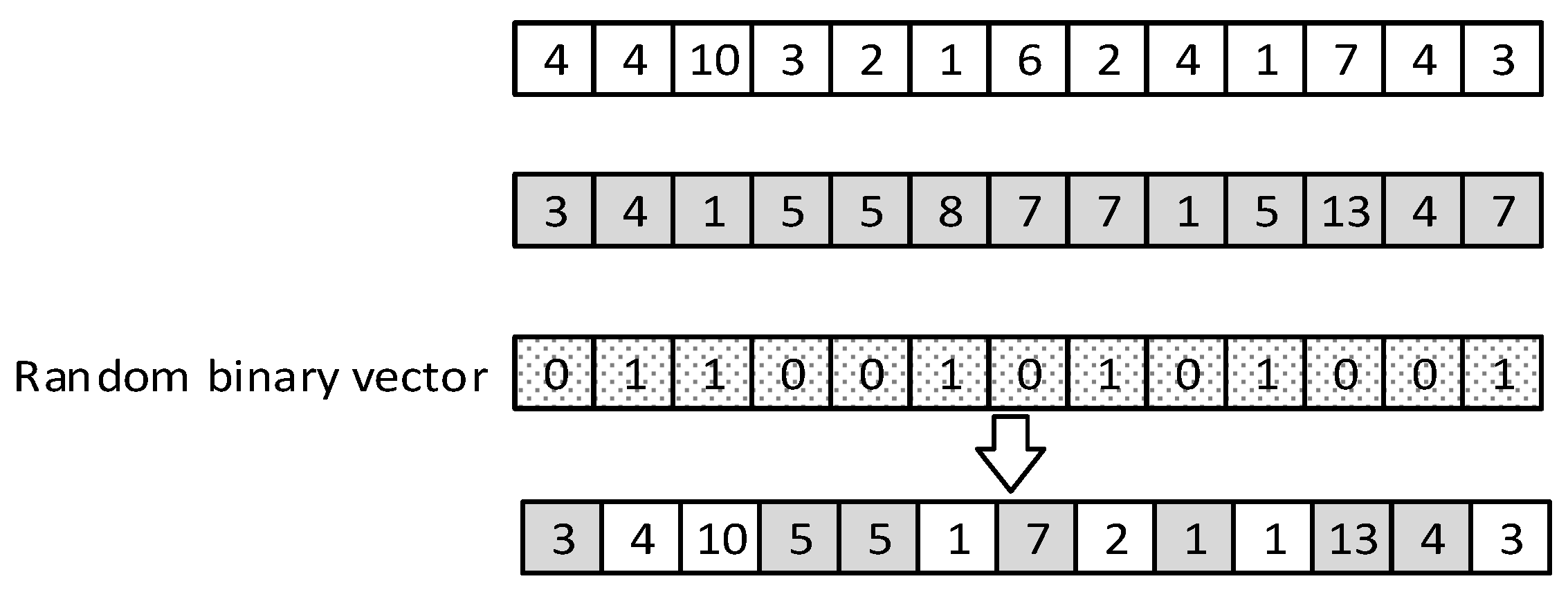
5.3.2. Crossover Operators
5.3.3. Mutation Operators
5.4. Combining Local Search (CLS)
5.5. Decomposing Local Search (DLS)
6. Experimental Design
6.1. Benchmark Problems
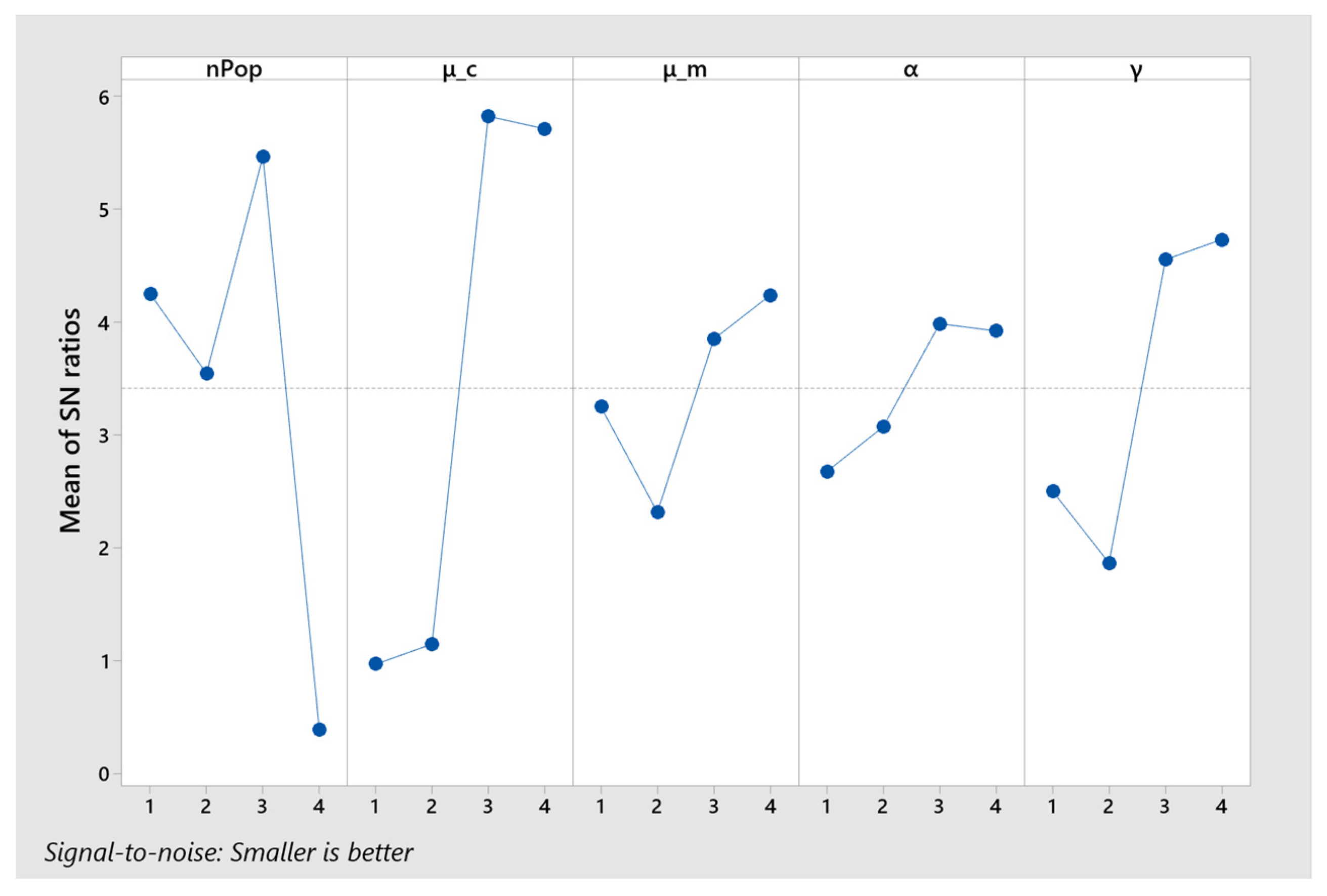
6.2. Parameter Settings
6.3. Computational Results
7. Managerial Insights
8. Conclusions and Discussion
Author Contributions
Funding
Data Availability Statement
Conflicts of Interest
Appendix A
| Algorithm A1: p-median based heuristic. |
| Inputs: A set of vertexes . A set of edge . The distance matrix corresponding to the 1: Set 2: While there exist feasible solutions Do 3: Solve the -median model 4: Solve the PTAP 5: 6: End While Output: The solution corresponding to the that resulted in the minimum objective function value in the PTAP |
| Algorithm A2: Combining Local Search (CLS). |
| 1: Extract the initial number of containers, , for a given solution 2: 3: While 4: For To Do 5: Calculate using Equations (12) and (13) 6: End For 7: For To 3 Do 8: If Then 9: Perform random walk on and obtain local optimum 10: Else If 11: Walk 1: combine the two containers with the lowest and obtain local optimum 12: Else If 13: Walk 2: combine the two containers with the highest and obtain local optimum 14: Else If 15: Walk 3: combine the containers with the lowest and the highest and obtain local optimum 16: End If 17: If Then 18: Perform the repairing mechanism 19: End If 20: End For 21: Add the best solution among , , and to the current population 22: 23: End While |
| Algorithm A3: Decomposing Local Search (DLS). |
| 1: Extract the initial number of containers for a given solution 2: 3: While 4: For To except peel packs Do 5: Calculate using Equation (12) 6: End For 7: Select the container with the lowest 8: For all instruments in tray 9: Calculate using Equation (14) 10: End For 11: For To 2 Do 12: If Then 13: Random walk: Generate a new solution by randomly selecting an instrument and putting it in a peel pack 14: Else If 15: Walk 1: Generate a new solution by putting the instrument with the lowest in a new container as a peel pack 16: Else If 17: Walk 2: Generate a new solution by putting the instrument with the highest in a new container as a peel pack 18: End If 19: End For 20: Select the container with the highest 21: For all instruments in tray 22: Calculate using Equation (14) 23: End For 24: For To 4 Do 25: If Then 26: Random walk: Generate a new solution by randomly selecting an instrument and putting it in a peel pack 27: Else If 28: Walk 1: Generate a new solution by putting the instrument with the lowest in a new container as a peel pack 29: Else If 30: Walk 2: Generate a new solution by putting the instrument with the highest in a new container as a peel pack 31: End If 32: End For 33: Add the best solution among , , , and to the current population 34: 35: End While |

| Instrument | ||||||||||||||
|---|---|---|---|---|---|---|---|---|---|---|---|---|---|---|
| 1 | 2 | 3 | 4 | 5 | 6 | 7 | 8 | 9 | 10 | 11 | 12 | 13 | ||
| Instrument | 1 | 3.00 | 6.29 | 9.55 | 7.67 | 6.00 | 7.66 | 6.67 | 6.24 | 7.93 | 6.50 | 6.36 | 10.69 | 6.30 |
| 2 | 6.29 | 0.50 | 6.27 | 3.39 | 1.02 | 5.29 | 2.23 | 1.24 | 4.53 | 1.50 | 1.36 | 8.58 | 1.82 | |
| 3 | 9.55 | 6.27 | 2.76 | 5.99 | 5.53 | 8.22 | 6.36 | 5.63 | 7.43 | 5.55 | 5.54 | 8.89 | 6.09 | |
| 4 | 7.67 | 3.39 | 5.99 | 1.28 | 2.57 | 6.59 | 3.75 | 2.80 | 5.00 | 2.71 | 2.67 | 8.37 | 3.31 | |
| 5 | 6.00 | 1.02 | 5.53 | 2.57 | 0.01 | 4.69 | 1.40 | 0.26 | 3.99 | 0.52 | 0.38 | 8.01 | 0.94 | |
| 6 | 7.66 | 5.29 | 8.22 | 6.59 | 4.69 | 2.34 | 5.40 | 4.80 | 7.51 | 5.18 | 5.04 | 9.61 | 5.19 | |
| 7 | 6.67 | 2.23 | 6.36 | 3.75 | 1.40 | 5.40 | 0.69 | 1.56 | 4.81 | 1.88 | 1.74 | 8.69 | 2.25 | |
| 8 | 6.24 | 1.24 | 5.63 | 2.80 | 0.26 | 4.80 | 1.56 | 0.12 | 4.22 | 0.74 | 0.60 | 8.05 | 1.16 | |
| 9 | 7.93 | 4.53 | 7.43 | 5.00 | 3.99 | 7.51 | 4.81 | 4.22 | 1.99 | 4.10 | 4.07 | 9.86 | 4.77 | |
| 10 | 6.50 | 1.50 | 5.55 | 2.71 | 0.52 | 5.18 | 1.88 | 0.74 | 4.10 | 0.25 | 0.77 | 8.03 | 1.42 | |
| 11 | 6.36 | 1.36 | 5.54 | 2.67 | 0.38 | 5.04 | 1.74 | 0.60 | 4.07 | 0.77 | 0.18 | 8.02 | 1.28 | |
| 12 | 10.69 | 8.58 | 8.89 | 8.37 | 8.01 | 9.61 | 8.69 | 8.05 | 9.86 | 8.03 | 8.02 | 4.00 | 8.25 | |
| 13 | 6.30 | 1.82 | 6.09 | 3.31 | 0.94 | 5.19 | 2.25 | 1.16 | 4.77 | 1.42 | 1.28 | 8.25 | 0.46 | |
| Experiment | Parameter’s Level | Cost ($) | Time (s) | Ncost | Ntime | Response | ||||
|---|---|---|---|---|---|---|---|---|---|---|
| 1 | 1 | 1 | 1 | 1 | 1 | 40.24 | 12.86 | 1.00 | 0.00 | 1.00 |
| 2 | 1 | 2 | 2 | 2 | 2 | 40.19 | 21.60 | 0.80 | 0.32 | 1.12 |
| 3 | 1 | 3 | 3 | 3 | 3 | 40.04 | 16.03 | 0.25 | 0.12 | 0.36 |
| 4 | 1 | 4 | 4 | 4 | 4 | 40.01 | 18.19 | 0.15 | 0.19 | 0.35 |
| 5 | 2 | 1 | 2 | 3 | 4 | 40.12 | 20.21 | 0.54 | 0.27 | 0.80 |
| 6 | 2 | 2 | 1 | 4 | 3 | 40.04 | 25.84 | 0.25 | 0.47 | 0.73 |
| 7 | 2 | 3 | 4 | 1 | 2 | 40.09 | 17.04 | 0.44 | 0.15 | 0.60 |
| 8 | 2 | 4 | 3 | 2 | 1 | 40.09 | 16.24 | 0.44 | 0.12 | 0.56 |
| 9 | 3 | 1 | 3 | 4 | 2 | 40.06 | 24.11 | 0.35 | 0.41 | 0.76 |
| 10 | 3 | 2 | 4 | 3 | 1 | 40.00 | 28.37 | 0.09 | 0.57 | 0.65 |
| 11 | 3 | 3 | 1 | 2 | 4 | 39.99 | 21.55 | 0.05 | 0.32 | 0.37 |
| 12 | 3 | 4 | 2 | 1 | 3 | 39.97 | 25.00 | 0.00 | 0.44 | 0.44 |
| 13 | 4 | 1 | 4 | 2 | 3 | 39.99 | 40.25 | 0.05 | 1.00 | 1.05 |
| 14 | 4 | 2 | 3 | 1 | 4 | 40.13 | 27.20 | 0.58 | 0.52 | 1.10 |
| 15 | 4 | 3 | 2 | 4 | 1 | 40.06 | 26.97 | 0.35 | 0.52 | 0.86 |
| 16 | 4 | 4 | 1 | 3 | 2 | 40.05 | 27.70 | 0.29 | 0.54 | 0.84 |


| Instruments | Containers | |||||||||||||
|---|---|---|---|---|---|---|---|---|---|---|---|---|---|---|
| 1 | 2 | 3 | 4 | 5 | 6 | 7 | 8 | 9 | 10 | 11 | 12 | 13 | 14 | |
| 1 | 1 | |||||||||||||
| 2 | 1 | |||||||||||||
| 3 | 1 | |||||||||||||
| 4 | 1 | |||||||||||||
| 5 | 1 | |||||||||||||
| 6 | 1 | |||||||||||||
| 7 | 1 | |||||||||||||
| 8 | 1 | |||||||||||||
| 9 | 1 | |||||||||||||
| 10 | 1 | |||||||||||||
| 11 | 1 | |||||||||||||
| 12 | 1 | |||||||||||||
| 13 | 1 | |||||||||||||
| 14 | 1 | |||||||||||||
| 15 | 1 | 1 | ||||||||||||
| 16 | 1 | 1 | ||||||||||||
| 17 | 1 | 1 | ||||||||||||
| 18 | 1 | 1 | ||||||||||||
| 19 | 1 | 1 | ||||||||||||
| 20 | 1 | 1 | ||||||||||||
| 21 | 1 | |||||||||||||
| 22 | 1 | 1 | ||||||||||||
| 23 | 1 | 1 | ||||||||||||
| 24 | 1 | 1 | ||||||||||||
| 25 | 1 | 1 | ||||||||||||
| 26 | 1 | 1 | ||||||||||||
| 27 | 1 | 1 | ||||||||||||
| 28 | 1 | 1 | ||||||||||||
| 29 | 1 | 1 | ||||||||||||
| 30 | 1 | 1 | ||||||||||||
| 31 | 1 | 1 | ||||||||||||
| 32 | 1 | 1 | ||||||||||||
| 33 | 1 | 1 | ||||||||||||
| 34 | 1 | 1 | ||||||||||||
| 35 | 1 | 1 | ||||||||||||
| 36 | 2 | |||||||||||||
| 37 | 1 | 1 | ||||||||||||
| 38 | 1 | 1 | ||||||||||||
| 39 | 2 | |||||||||||||
| 40 | 1 | 1 | ||||||||||||
| 41 | 1 | 1 | ||||||||||||
| 42 | 1 | 1 | ||||||||||||
| 43 | 1 | 1 | ||||||||||||
| 44 | 1 | 1 | ||||||||||||
| 45 | 1 | 1 | ||||||||||||
| 46 | 1 | 1 | ||||||||||||
| 47 | 1 | 1 | ||||||||||||
| 48 | 1 | 1 | ||||||||||||
| 49 | 1 | 1 | ||||||||||||
| 50 | 1 | 1 | ||||||||||||
| 51 | 1 | 1 | ||||||||||||
| 52 | 1 | 1 | ||||||||||||
| 53 | 1 | 1 | ||||||||||||
| 54 | 2 | |||||||||||||
| 55 | 1 | 1 | ||||||||||||
| 56 | 2 | |||||||||||||
| 57 | 1 | 1 | ||||||||||||
| 58 | 1 | 1 | ||||||||||||
| 59 | 2 | |||||||||||||
| 60 | 1 | 1 | ||||||||||||
| 61 | 1 | 1 | ||||||||||||
| 62 | 1 | 1 | ||||||||||||
| 63 | 1 | 1 | ||||||||||||
| 64 | 1 | 1 | ||||||||||||
| 65 | 2 | |||||||||||||
| 66 | 1 | |||||||||||||
| 67 | 1 | 1 | ||||||||||||
| 68 | 1 | 1 | ||||||||||||
| 69 | 1 | 1 | ||||||||||||
| 70 | 1 | 1 | ||||||||||||
| 71 | 1 | 1 | ||||||||||||
| 72 | 1 | 1 | ||||||||||||
| 73 | 1 | 1 | ||||||||||||
| 74 | 1 | 1 | ||||||||||||
| 75 | 1 | 1 | ||||||||||||
| 76 | 1 | 1 | ||||||||||||
References
- CMS. National Health Expenditure Projections 2019–2028, Office. 2020, 1–17. Available online: https://www.cms.gov/Research-Statistics-Data-and-Systems/Statistics-Trends-and-Reports/NationalHealthExpendData/NationalHealthAccountsProjected (accessed on 13 January 2022).
- Ahmadi, E.; Masel, D.T.; Schwerha, D.; Hostetler, S. A bi-objective optimization approach for configuring surgical trays with ergonomic risk consideration. IISE Trans. Healthc. Syst. Eng. 2019, 9, 327–341. [Google Scholar] [CrossRef]
- Schoenfelder, J.; Kohl, S.; Glaser, M.; McRae, S.; Brunner, J.O.; Koperna, T. Simulation-based evaluation of operating room management policies. BMC Health Serv. Res. 2021, 21, 271. [Google Scholar] [CrossRef]
- Görgülü, B.; Sarhangian, V. Newsvendor Approach to Design of Surgical Preference Cards. Serv. Sci. 2022, 14, 213–230. [Google Scholar] [CrossRef]
- Ahmadi, E.; Masel, D.T.; Hostetler, S. A robust stochastic decision-making model for inventory allocation of surgical supplies to reduce logistics costs in hospitals: A case study. Oper. Oper. Res. Health Care 2019, 20, 33–44. [Google Scholar] [CrossRef]
- Stockert, E.W.; Langerman, A. Assessing the magnitude and costs of intraoperative inefficiencies attributable to surgical instrument trays. J. Am. Coll. Surg. 2014, 219, 646–655. [Google Scholar] [CrossRef]
- Mhlaba, J.M.; Stockert, E.W.; Coronel, M.; Langerman, A.J. Surgical instrumentation: The true cost of instrument trays and a potential strategy for optimization. J. Hosp. Adm. 2015, 4, 82. [Google Scholar] [CrossRef]
- Koyle, M.A.; AlQarni, N.; Odeh, R.; Butt, H.; Alkahtani, M.M.; Konstant, L.; Pendergast, L.; Koyle, L.C.; Baker, G.R. Reduction and standardization of surgical instruments in pediatric inguinal hernia repair. J. Pediatr. Urol. 2018, 14, 20–24. [Google Scholar] [CrossRef]
- Farrokhi, F.R.; Gunther, M.; Williams, B.; Blackmore, C.C. Application of lean methodology for improved quality and efficiency in operating room instrument availability. J. Healthc. Qual. 2015, 37, 277–286. [Google Scholar] [CrossRef] [PubMed]
- Harvey, L.; Slocum, P.; Heft, J.; Van Meter, M.; Lovett, B.; Adam, R. Gynecologic Surgery Instrument Trays: Leveraging Surgeon Knowledge to Improve Supply Chain Efficiency. J. Gynecol. Surg. 2017, 33, 180–183. [Google Scholar] [CrossRef]
- Nast, K.; Swords, K. Decreasing operating room costs via reduction of surgical instruments. J. Pediatr. Urol. 2019, 15, 153.e1–153.e6. [Google Scholar] [CrossRef]
- Choobineh, A.; Movahed, M.; Tabatabaie, S.H.; Kumashiro, M. Perceived Demands and Musculoskeletal Disorders in Operating Room Nurses of Shiraz City Hospitals. Ind. Health 2010, 48, 74–84. [Google Scholar] [CrossRef] [PubMed]
- Seavey, R. Packaging for Sterilization: It’s not just a box, a bag or gift wrapping! Manag. Infect. Control. 2008, 8, 82–97. [Google Scholar]
- Sheikhzadeh, A.; Gore, C.; Zuckerman, J.D.; Nordin, M. Perioperating nurses and technicians’ perceptions of ergonomic risk factors in the surgical environment. Appl. Ergon. 2009, 40, 833–839. [Google Scholar] [CrossRef] [PubMed]
- Choi, S.D. A Review of the Ergonomic Issues in the Laparoscopic Operating Room. J. Healthc. Eng. 2012, 3, 587–604. [Google Scholar] [CrossRef]
- Morris, L.F.; Arenas, M.A.R.; Cerny, J.; Berger, J.S.; Borror, C.M.; Ong, M.; Cayo, A.K.; Graham, P.H.; Grubbs, E.G.; Lee, J.E.; et al. Streamlining variability in hospital charges for standard thyroidectomy: Developing a strategy to decrease waste. Surgery 2014, 156, 1441–1449. [Google Scholar] [CrossRef] [PubMed]
- Dollevoet, T.; van Essen, J.T.; Glorie, K.M. Solution methods for the tray optimization problem. Eur. J. Oper. Res. 2018, 271, 1070–1084. [Google Scholar] [CrossRef]
- Ahmadi, E.; Masel, D.T.; Metcalf, A.Y.; Schuller, K. Inventory management of surgical supplies and instruments in hospitals: A literature review. Health Syst. 2018, 8, 134–151. [Google Scholar] [CrossRef]
- Van de Klundert, J.; Muls, P.; Schadd, M. Optimizing sterilization logistics in hospitals. Health Care Manag. Sci. 2008, 11, 23–33. [Google Scholar] [CrossRef]
- Florijn, E.P. Optimisation of the Distribution of Surgical Instruments over Trays: Cost Effectiveness and Quality Improvement of an Operating Theatre. Master’s Thesis, University of Twente, Enschede, The Netherlands, 2008. [Google Scholar]
- Reymondon, F.; Pellet, B.; Marcon, E. Optimization of hospital sterilization costs proposing new grouping choices of medical devices into packages. Int. J. Prod. Econ. 2008, 112, 326–335. [Google Scholar] [CrossRef]
- Dobson, G.; Seidmann, A.; Tilson, V.; Froix, A. Configuring surgical instrument trays to reduce costs. IIE Trans. Healthc. Syst. Eng. 2015, 5, 225–237. [Google Scholar] [CrossRef]
- Dos Santos, B.M.; Fogliatto, F.S.; Zani, C.M.; Peres, F.A.P. Approaches to the rationalization of surgical instrument trays: Scoping review and research agenda. BMC Health Serv. Res. 2021, 21, 163. [Google Scholar] [CrossRef]
- Harris, S.; Claudio, D. A Goal Programming Approach to the Tray Optimization Problem. In IIE Annual Conference. Proceedings; Institute of Industrial and Systems Engineers (IISE): Peachtree Corners, GA, USA, 2021; pp. 680–685. [Google Scholar]
- Deshpande, V.; Mundru, N.; Rath, S.; Knowles, M.; Rowe, D.; Wood, B.C. Data-Driven Surgical Tray Optimization to Improve Operating Room Efficiency. Oper. Res. 2023. [Google Scholar] [CrossRef]
- AAMI. Comprehensive Guide to Steam Sterilzation and Sterility Assurance in Health Care Facilities; AAMI: Melbourne, VIC, Australia, 2006. [Google Scholar]
- Karp, R.M. Reducibility among combinatorial problems. In Complexity of Computer Computations; Springer: Berlin/Heidelberg, Germany, 1972; pp. 85–103. [Google Scholar]
- Berman, O.; Wang, J. The network p-median problem with discrete probabilistic demand weights. Comput. Oper. Res. 2010, 37, 1455–1463. [Google Scholar] [CrossRef]
- Mladenović, N.; Brimberg, J.; Hansen, P.; Moreno-Pérez, J.A. The p-median problem: A survey of metaheuristic approaches. Eur. J. Oper. Res. 2007, 179, 927–939. [Google Scholar] [CrossRef]
- Kusiak, A. The generalized group technology concept. Int. J. Prod. Res. 1987, 25, 561–569. [Google Scholar] [CrossRef]
- Wang, J.; Roze, C. Formation of Machine Cells and Part Families in Cellular Manufacturing: A Linear Integer Programming Approach. In Proceedings of the 1994 IEEE International Conference on Industrial Technology—ICIT ’94, Guangzhou, China, 5–9 December 1994; pp. 350–354. [Google Scholar]
- Hassanzadeh, R.; Mahdavi, I.; Mahdavi-Amiri, N.; Tajdin, A. A genetic algorithm for solving fuzzy shortest path problems with mixed fuzzy arc lengths. Math. Comput. Model. 2013, 57, 84–99. [Google Scholar] [CrossRef]
- Ahmadi, E.; Süer, G.A.; Al-Ogaili, F. Solving Stochastic Shortest Distance Path Problem by Using Genetic Algorithms. Procedia Comput. Sci. 2018, 140, 79–86. [Google Scholar] [CrossRef]
- Ahmadi, E.; Masel, D.T.; Hostetler, S.; Maihami, R.; Ghalehkhondabi, I. A centralized stochastic inventory control model for perishable products considering age-dependent purchase price and lead time. TOP 2020, 28, 231–269. [Google Scholar] [CrossRef]
- Vahdani, B.; Soltani, M.; Yazdani, M.; Mousavi, S.M. A three level joint location-inventory problem with correlated demand, shortages and periodic review system: Robust meta-heuristics. Comput. Ind. Eng. 2017, 109, 113–129. [Google Scholar] [CrossRef]
- Ahmadi, E.; Mosadegh, H.; Maihami, R.; Ghalehkhondabi, I.; Sun, M.; Süer, G.A. Intelligent inventory management approaches for perishable pharmaceutical products in a healthcare supply chain. Comput. Oper. Res. 2022, 147, 105968. [Google Scholar] [CrossRef]
- Talbi, E.-G. Metaheuristics: From Design to Implementation; John Wiley & Sons: Hoboken, NJ, USA, 2009. [Google Scholar]
- Asefi, H.; Jolai, F.; Rabiee, M.; Araghi, M.E.T. A hybrid NSGA-II and VNS for solving a bi-objective no-wait flexible flowshop scheduling problem. Int. J. Adv. Manuf. Technol. 2014, 75, 1017–1033. [Google Scholar] [CrossRef]
- Aghaaminiha, M.; Ghanadian, S.A.; Ahmadi, E.; Farnoud, A.M. A machine learning approach to estimation of phase diagrams for three- component lipid mixtures. Biochim. Biophys. Acta BBA-Biomembr. 2020, 1862, 183350. [Google Scholar] [CrossRef] [PubMed]
- Diamant, A.; Milner, J.; Quereshy, F.; Xu, B. Inventory management of reusable surgical supplies. Health Care Manag. Sci. 2017, 21, 439–459. [Google Scholar] [CrossRef] [PubMed]
- John-Baptiste, A.; Sowerby, L.; Chin, C.; Martin, J.; Rotenberg, B. Comparing surgical trays with redundant instruments with trays with reduced instruments: A cost analysis. CMAJ Open 2016, 4, E404–E408. [Google Scholar] [CrossRef] [PubMed]


| Surgeon-Procedures | Instrument | ||||
|---|---|---|---|---|---|
| 1 | 2 | 3 | 4 | 5 | |
| 1 | 0 | 2 | 0 | 3 | 1 |
| 2 | 0 | 1 | 3 | 0 | 1 |
| 3 | 2 | 3 | 2 | 1 | 2 |
| 4 | 1 | 1 | 1 | 0 | 2 |
| 5 | 2 | 2 | 1 | 0 | 2 |
| 6 | 2 | 0 | 2 | 1 | 0 |
| Surgeon-Procedures | Instrument | ||||||||||||
|---|---|---|---|---|---|---|---|---|---|---|---|---|---|
| 1 | 2 | 3 | 4 | 5 | |||||||||
| 1 | 0 | 0 | 1 | 1 | 0 | 0 | 0 | 0 | 1 | 1 | 1 | 1 | 0 |
| 2 | 0 | 0 | 1 | 0 | 0 | 1 | 1 | 1 | 0 | 0 | 0 | 1 | 0 |
| 3 | 1 | 1 | 1 | 1 | 1 | 1 | 1 | 0 | 1 | 0 | 0 | 1 | 1 |
| 4 | 1 | 0 | 1 | 0 | 0 | 1 | 0 | 0 | 0 | 0 | 0 | 1 | 1 |
| 5 | 1 | 1 | 1 | 1 | 0 | 1 | 0 | 0 | 0 | 0 | 0 | 1 | 1 |
| 6 | 1 | 1 | 0 | 0 | 0 | 1 | 1 | 0 | 1 | 0 | 0 | 0 | 0 |
| Proc. | Instrument | ||||||||||||
|---|---|---|---|---|---|---|---|---|---|---|---|---|---|
| 1 | 2 | 3 | 4 | 5 | |||||||||
| 1 | 0.00 | 0.00 | 0.95 | 0.70 | 0.00 | 0.00 | 0.00 | 0.00 | 0.76 | 0.25 | 0.18 | 0.95 | 0.00 |
| 2 | 0.00 | 0.00 | 0.56 | 0.00 | 0.00 | 0.48 | 0.26 | 0.12 | 0.00 | 0.00 | 0.00 | 0.80 | 0.00 |
| 3 | 0.80 | 0.15 | 0.70 | 0.53 | 0.01 | 0.60 | 0.18 | 0.00 | 0.45 | 0.00 | 0.00 | 0.75 | 0.14 |
| 4 | 0.90 | 0.00 | 0.40 | 0.00 | 0.00 | 0.68 | 0.00 | 0.00 | 0.00 | 0.00 | 0.00 | 0.85 | 0.12 |
| 5 | 0.45 | 0.15 | 0.15 | 0.05 | 0.00 | 0.19 | 0.00 | 0.00 | 0.00 | 0.00 | 0.00 | 0.65 | 0.20 |
| 6 | 0.85 | 0.20 | 0.00 | 0.00 | 0.00 | 0.39 | 0.25 | 0.00 | 0.78 | 0.00 | 0.00 | 0.00 | 0.00 |
| Container Type | Included Instruments in the Container * | Container Type | Container’s Contribution () |
|---|---|---|---|
| 1 | Tray | 155.4 | |
| 2 | Tray | 7.8 | |
| 3 | Tray | 99.4 | |
| 4 | Tray | 667.1 | |
| 6 | Peel pack | 13.8 | |
| 7 | Peel pack | 3.6 | |
| 10 | Peel pack | 55.2 |
| Dataset Name | Number of Instances | Number of Surgeons | Number of Procedures | Number of Unique Instruments | Total Number of Instruments |
|---|---|---|---|---|---|
| VLD | 5 | 2 | 3 | 5 | 13 |
| 1S-7P | 5 | 1 | 7 | 76 | 136 |
| 2S-7P | 5 | 2 | 7 | 76 | 136 |
| 5S-7P | 5 | 5 | 7 | 76 | 250 |
| Level | |||||
|---|---|---|---|---|---|
| 1 | 30 | 0.40 | 0.50 | 0.20 | 0.20 |
| 2 | 50 | 0.50 | 0.60 | 0.40 | 0.40 |
| 3 | 70 | 0.60 | 0.70 | 0.60 | 0.60 |
| 4 | 90 | 0.70 | 0.80 | 0.80 | 0.80 |
| Dataset | Instance # | B-BB | H-GA-CD | ||||||
|---|---|---|---|---|---|---|---|---|---|
| Average | S.D. | Best | Time | Average | S.D. | Best | Time | ||
| VLD | 1 | 46.7 | 4.3 | 44.7 | 2064.8 | 40.0 | 0.2 | 39.9 | 24.3 |
| 2 | 58.4 | 6.8 | 46.6 | 915.10 | 37.4 | 0.1 | 37.3 | 23.0 | |
| 3 | 43.9 | 2.4 | 42.8 | 2095.9 | 31.1 | 0.4 | 30.9 | 26.7 | |
| 4 | 40.4 | 8.9 | 34.0 | 1773.6 | 35.0 | 0.5 | 34.7 | 24.8 | |
| 5 | 43.4 | 5.2 | 37.4 | 1240.0 | 32.9 | 0.0 | 32.9 | 28.4 | |
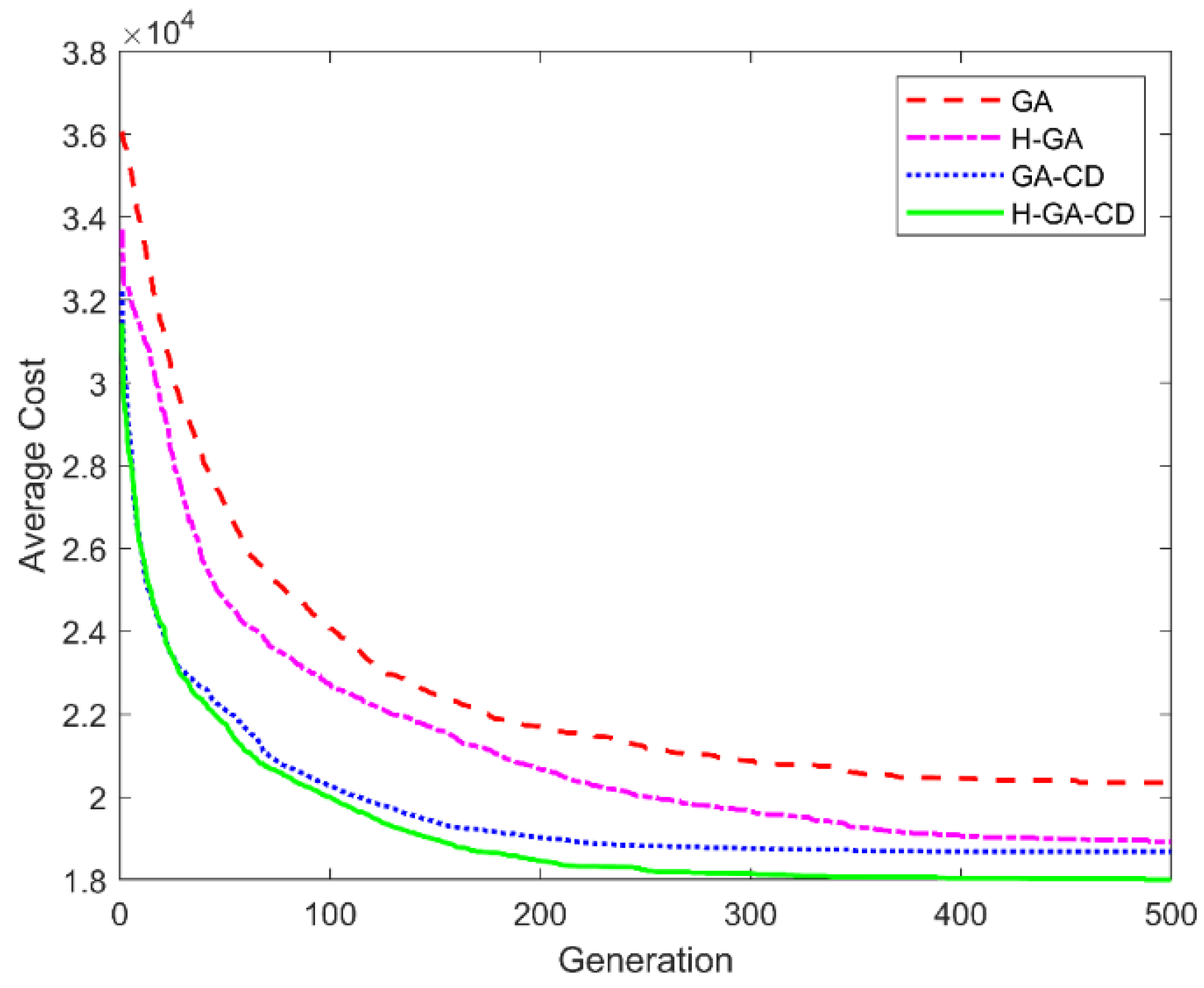
| Dataset | Instance # | GA | H-GA | GA-CD | H-GA-CD | ||||||||||||
|---|---|---|---|---|---|---|---|---|---|---|---|---|---|---|---|---|---|
| Ave. | S.D. | Best | Time | Ave. | S.D. | Best | Time | Ave. | S.D. | Best | Time | Ave. | S.D. | Best | Time | ||
| 1S-7P | 1 | 10,057 | 466 | 9560 | 1897 | 8739 | 33 | 8716 | 2093 | 8744 | 195 | 8520 | 1772 | 8757 | 189 | 8538 | 2147 |
| 2 | 9889 | 364 | 9341 | 1685 | 8973 | 223 | 8765 | 2236 | 8781 | 139 | 8573 | 1763 | 8720 | 78 | 8582 | 1621 | |
| 3 | 9717 | 357 | 9131 | 1712 | 8813 | 245 | 8509 | 2058 | 8776 | 172 | 8489 | 1721 | 8835 | 232 | 8629 | 1682 | |
| 4 | 8341 | 330 | 7855 | 1723 | 7514 | 284 | 7229 | 2051 | 7446 | 152 | 7260 | 1994 | 7316 | 151 | 7168 | 2134 | |
| 5 | 8370 | 255 | 7966 | 1711 | 7849 | 486 | 7500 | 2443 | 7425 | 122 | 7221 | 2206 | 7448 | 102 | 7310 | 1981 | |
| 2S-7P | 1 | 19,951 | 449 | 19,505 | 5072 | 18,984 | 125 | 18,841 | 5256 | 18,046 | 252 | 17,769 | 7871 | 18,864 | 114 | 18,786 | 7649 |
| 2 | 20,190 | 345 | 19,861 | 5095 | 19,420 | 256 | 19,105 | 4945 | 17,309 | 366 | 16,875 | 8966 | 19,285 | 272 | 19,048 | 8218 | |
| 3 | 19,921 | 381 | 19,380 | 4918 | 18,357 | 221 | 18,093 | 4865 | 17,502 | 309 | 17,225 | 7940 | 18,439 | 143 | 18,223 | 7956 | |
| 4 | 20,475 | 391 | 19,869 | 5057 | 19,878 | 600 | 19,348 | 4816 | 17,893 | 336 | 17,506 | 8031 | 19,502 | 147 | 19,332 | 7824 | |
| 5 | 20,198 | 376 | 19,620 | 4927 | 18,617 | 145 | 18,485 | 4592 | 17,619 | 245 | 17,443 | 7753 | 19,351 | 142 | 19,188 | 7302 | |
| 5S-7P | 1 | 84,102 | 1068 | 82,810 | 79,024 | 90,673 | 4165 | 86,756 | 81,111 | 82,950 | 4161 | 78,972 | 165,620 | 83,409 | 4269 | 77,557 | 166,985 |
| 2 | 85,551 | 1243 | 84,536 | 78,901 | 90,216 | 1796 | 88,398 | 84,093 | 82,792 | 2326 | 80,335 | 172,940 | 82,432 | 2153 | 79,260 | 165,187 | |
| 3 | 85,042 | 1895 | 82,728 | 78,869 | 89,550 | 1744 | 87,570 | 82,359 | 82,269 | 3698 | 78,203 | 169,844 | 80,998 | 2800 | 76,270 | 167,017 | |
| 4 | 85,270 | 1848 | 83,249 | 77,985 | 91,259 | 4093 | 86,618 | 80,321 | 82,731 | 2868 | 78,724 | 171,444 | 79,654 | 1596 | 78,274 | 165,616 | |
| 5 | 85,411 | 1052 | 84,432 | 77,893 | 88,867 | 3434 | 85,064 | 81,974 | 83,674 | 2607 | 79,609 | 168,058 | 83,248 | 2527 | 80,420 | 163,162 | |
| Dataset | GA | H-GA | GA-CD | H-GA-CD |
|---|---|---|---|---|
| GA | - | - | - | - |
| H-GA | 0.585 (no significant difference) | - | - | - |
| GA-CD | 0.013 (GA-CD performs better) | 0.021 (GA-CD performs better) | - | - |
| H-GA-CD | 0.018 (H-GA-CD performs better) | 0.252 (no significant difference) | 0.358 (no significant difference) | - |
| Surgeon | Procedure | Containers | |||||||||||||
|---|---|---|---|---|---|---|---|---|---|---|---|---|---|---|---|
| 1 | 2 | 3 | 4 | 5 | 6 | 7 | 8 | 9 | 10 | 11 | 12 | 13 | 14 | ||
| Surgeon 1 | Mediport insertion | 100% | 100% | 53% | 19% | 99% | 9% | 77% | 25% | 51% | 82% | ||||
| Excision of small lesion | 100% | 100% | 76% | ||||||||||||
| Lap appendectomy | 100% | 100% | 100% | 32% | 95% | 92% | 99% | 2% | 72% | ||||||
| Lap cholecystectomy | 100% | 100% | 67% | 99% | 50% | ||||||||||
| Lap ventral hernia repair | 100% | 100% | 99% | 49% | 67% | 60% | 97% | 75% | 12% | 39% | 11% | ||||
| Open hernia repair | 100% | 100% | 100% | 99% | 100% | 100% | |||||||||
| Bowel resection | 100% | 100% | 100% | 86% | 100% | 96% | 100% | 48% | 35% | 56% | 20% | 55% | 4% | ||
| Surgeon 2 | Mediport insertion | 100% | 100% | 41% | 26% | 69% | 6% | 98% | 39% | ||||||
| Excision of small lesion | 100% | 100% | |||||||||||||
| Lap appendectomy | 97% | 100% | 100% | 16% | 11% | 84% | |||||||||
| Lap cholecystectomy | 100% | 100% | 2% | ||||||||||||
| Lap ventral hernia repair | 100% | 100% | 59% | 33% | 33% | 95% | 75% | 55% | |||||||
| Open hernia repair | 100% | 100% | 99% | 100% | 68% | 99% | |||||||||
| Bowel resection | 100% | 100% | 100% | 37% | 98% | 100% | 98% | 21% | 74% | 98% | 9% | ||||
| Number of instruments | 27 | 23 | 13 | 11 | 11 | 9 | 9 | 8 | 7 | 6 | 5 | 3 | 3 | 1 | |
| Weight (lb.) | 14.17 | 11.56 | 8.06 | 5.67 | 6.6 | 3.16 | 5.43 | 3.62 | 3.7 | 2.52 | 1.4 | 1.6 | 0.89 | 0.56 | |
| Resterilization cost per procedure if the container is opened | $10.80 | $9.20 | $5.20 | $4.40 | $4.40 | $3.60 | $3.60 | $3.20 | $2.80 | $2.40 | $2.00 | $1.20 | $1.20 | $0.80 | |
| Value of | 3 | 4 | 5 | 6 | 7 | 8 | 9 | 10 | 11 | 12 | 13 | 14 | 15 |
| Number of trays | 3 | 4 | 5 | 6 | 7 | 8 | 8 | 9 | 9 | 11 | 12 | 13 | 13 |
| Number of peel packs | 0 | 0 | 0 | 0 | 0 | 0 | 1 | 1 | 2 | 1 | 1 | 1 | 1 |
| $20,383 | $18,393 | $17,009 | $15,997 | $15,326 | $14,836 | $14,594 | $14,027 | $13,842 | $13,712 | $13,292 | $13,120 | $13,120 | |
| $0 | $0 | $0 | $0 | $0 | $0 | $1 | $16 | $60 | $1 | $3 | $1 | $1 | |
| $2132 | $2256 | $2849 | $3509 | $3948 | $3976 | $3982 | $4006 | $4067 | $4179 | $4552 | $4641 | $4641 | |
| $0 | $0 | $0 | $0 | $0 | $0 | $18 | $118 | $79 | $17 | $7 | $7 | $7 | |
| Total Cost | $22,514 | $20,649 | $19,858 | $19,506 | $19,274 | $18,812 | $18,595 | $18,167 | $18,048 | $17,909 | $17,853 | $17,769 | $17,769 |
| Cost Savings/ | $1866 | $790 | $353 | $232 | $462 | $218 | $428 | $118 | $139 | $56 | $84 | $0 |
Disclaimer/Publisher’s Note: The statements, opinions and data contained in all publications are solely those of the individual author(s) and contributor(s) and not of MDPI and/or the editor(s). MDPI and/or the editor(s) disclaim responsibility for any injury to people or property resulting from any ideas, methods, instructions or products referred to in the content. |
© 2023 by the authors. Licensee MDPI, Basel, Switzerland. This article is an open access article distributed under the terms and conditions of the Creative Commons Attribution (CC BY) license (https://creativecommons.org/licenses/by/4.0/).
Share and Cite
Ahmadi, E.; Masel, D.T.; Hostetler, S. A Data-Driven Decision-Making Model for Configuring Surgical Trays Based on the Likelihood of Instrument Usages. Mathematics 2023, 11, 2219. https://doi.org/10.3390/math11092219
Ahmadi E, Masel DT, Hostetler S. A Data-Driven Decision-Making Model for Configuring Surgical Trays Based on the Likelihood of Instrument Usages. Mathematics. 2023; 11(9):2219. https://doi.org/10.3390/math11092219
Chicago/Turabian StyleAhmadi, Ehsan, Dale T. Masel, and Seth Hostetler. 2023. "A Data-Driven Decision-Making Model for Configuring Surgical Trays Based on the Likelihood of Instrument Usages" Mathematics 11, no. 9: 2219. https://doi.org/10.3390/math11092219