A Novel Reconstruction of the Sparse-View CBCT Algorithm for Correcting Artifacts and Reducing Noise

Abstract

X-ray tomography is often affected by noise and artifacts during the reconstruction process, such as detector offset, calibration errors, metal artifacts, etc. Conventional algorithms, including FDK and SART, are unable to satisfy the sampling theorem requirements for 3D reconstruction under sparse-view constraints, exacerbating the impact of noise and artifacts. This paper proposes a novel 3D reconstruction algorithm tailored to sparse-view cone-beam computed tomography (CBCT). Drawing upon compressed sensing theory, we incorporate the weighted Schatten p-norm minimization (WSNM) algorithm for 2D image denoising and the adaptive steepest descent projection onto convex sets (ASD-POCS) algorithm, which employs a total variation (TV) regularization term. These inclusions serve to reduce noise and ameliorate artifacts. Our proposed algorithm extends the WSNM approach into three-dimensional space and integrates the ASD-POCS algorithm, enabling 3D reconstruction with digital brain phantoms, clinical medical data, and real projections from our portable CBCT system. The performance of our algorithm surpasses traditional methods when evaluated using root mean square error (RMSE), peak signal-to-noise ratio (PSNR), and structural similarity index measure (SSIM) metrics. Furthermore, our approach demonstrates marked enhancements in artifact reduction and noise suppression.

1. Introduction

CBCT is a CT-based imaging modality that enables three-dimensional visualization of an object using divergent X-rays emitted from a source. In CBCT, voxels are reconstructed from a series of projections captured at various angles around the object. Imaging processes in CBCT can be primarily categorized into analytical and iterative algorithms. Analytical algorithms, based on Radon transform and the central slice theorem, include Filtered Back Projection (FBP) and the Feldkamp–Davis–Kress (FDK) algorithm [1]. On the other hand, iterative algorithms, as described in [2], such as the simultaneous algebraic reconstruction technique (SART) and the ordered-subset simultaneous algebraic reconstruction technique (OS-SART), treat projection data as constraint conditions for reconstruction, building an iterative optimization objective function from discrete mathematical models and projection data. Although these classic algorithms have been successfully applied to full-view CBCT reconstruction, they struggle to address severe artifacts in sparse-view scenarios due to limitations in acquisition time and range. Consequently, reconstructing partial or global slice images of a target using incomplete projection data has become a research hotspot in the field of CT image reconstruction, emphasizing the importance of sparse projection.

Sparse-view [3] projection data do not comply with the Shannon sampling theorem [4], and conventional algorithms cannot resolve the issue. Donoho [5] and Candes [6] proposed compressed sensing (CS) theory in 2006, which posits that if a signal is sparse in a specific transformation domain, only a small portion of signal sampling is needed to accurately recover the original signal through solving an optimization problem. Sidky introduced the total variation (TV) regularization term, based on the prior knowledge of the gradient sparsity of CT reconstruction models, to obtain an incomplete projection data reconstruction model capable of addressing sparse projection data reconstruction with limited projection angles, and sparse or less-complete angle constraints. Inspired by CS theory, the literature [7] has made breakthroughs in utilizing sparse prior knowledge of total variation minimization of images. Combining the projection on convex sets algorithm with the adaptive steepest descent algorithm led to the development of the ASD-POCS method. Bian et al. first sampled the weight function in analytical methods to obtain a weight matrix for semi covering sparse angle CT reconstruction, then weighted the projection of the weight matrix and solved it using the ASD-POCS method. In machine learning, Yang et al. [8] proposed a convolutional neural network residual learning algorithm to correct artifacts in CBCT in 2020. The PSNR of the image corrected by this algorithm has increased by $15.4\%$. In 2021, Sori et al. [9] focused on learning local and global features of lung CT images, designing a dual-path convolutional neural network (CNN) model to effectively suppress noise artifacts in lung images. Wang et al. [10] proposed a dual-domain metal artifact correction network, combining projection and image domains. First, the damaged sine map is corrected, and then an end-to-end dual-domain network is used to sequentially process and analyze the input sine map and its corresponding reconstructed images. Dual-domain networks effectively improve the quality of reconstructed images and suppress metal artifacts.

Moreover, various types of noise, including streak noise and Poisson noise, affect sparse CBCT reconstruction. Streak noise in projections causes ring artifacts in reconstructed volumes, presenting as centered circles or half-circles [11]. Makinen et al. [12] proposed effective ring artifact attenuation through sinogram-domain collaborative filtering, presenting a multiscale architecture with a block-matching and 3D filtering (BM3D) image denoiser for correlated noise [13] at the core of the process. They provided state-of-the-art results in ring attenuation without introducing new artifacts around strong signal features, which is common with other popular ring removal algorithms. However, being based on a filter for 2D data applied to individual sinograms, it may cause discontinuities across the third dimension. To address this issue, Makinen et al. [14] proposed a 3D multiscale framework for streak attenuation through a specially designed collaborative filtering of correlated noise in volumetric data. They further proposed a distinct multiscale denoising step for attenuation of Poissonian noise. Utilizing the volumetric structure of the projection data, the fully automatic procedure offers improved feature preservation compared to 2-D denoising and avoids artifacts that arise from individual filtering of sinograms.

To tackle noise issues in sparse-view scenarios, this study explores the field of image and signal denoising, identifying that low-rank matrix approximation (LRMA) has gained considerable attention. The nuclear norm minimization and the Schatten p-norm ($0<p\le 1$) minimization [15] have been employed to solve LRMA. However, as these methods treat all singular values equally and shrink them with the same threshold, they result in poor edge preservation. To overcome this shortcoming, weighted nuclear norm minimization (WNNM) [16] and WSNM [17,18] are proposed, which shrink larger singular values less during rank minimization. WSNM is proven to be more effective, as it can be transformed into a series of independent non-convex lp-norm minimization problems and solved efficiently with a generalized soft-thresholding (GST) algorithm [19] in report [17].

Currently, the latest reconstruction methods primarily rely on machine learning techniques. However, the complexity of outdoor environments and the diversity of subjects can result in insufficient sample sizes, rendering the usage scenarios targeted in this paper inadequate to support machine learning applications. To reduce dependence on training data, we mainly adopt the compressive sensing theory reconstruction model and compare it with the sparse reconstruction algorithm that does not require training data for verification. Consequently, we propose a novel iterative algorithm for sparse-view CBCT reconstruction that corrects artifacts and reduces noise. Inspired by previous investigations [20], we introduce WSNM for quantifying self-similarity and reducing noise and ASD-POCS for solving the reconstruction problem of sparse projection data. Additionally, we fuse denoising voxels using the similarity coefficient based on WSNM, originally proposed for 2D image denoising. The proposed method combines the advantages of both techniques, reducing the impact of noise, decreasing the number of projections, and balancing noise suppression with structural information preservation. In simulation experiment 1, we obtained head phantom reconstruction using the proposed method with 90 projections. The root mean square error (RMSE), the structural similarity index (SSIM), and PSNR values were 0.00008, 44.54638, and 0.98968, respectively. In experiment 2, we used a publicly available CT dataset to reconstruct through 45 projections. In experiment 3, we used real walnut projections to reconstruct through 60 projections. Based on the quantitative evaluation of experimental results, the proposed method for sparse-view CBCT three-dimensional reconstruction outperforms traditional algorithms.

2. Reconstruction Methods

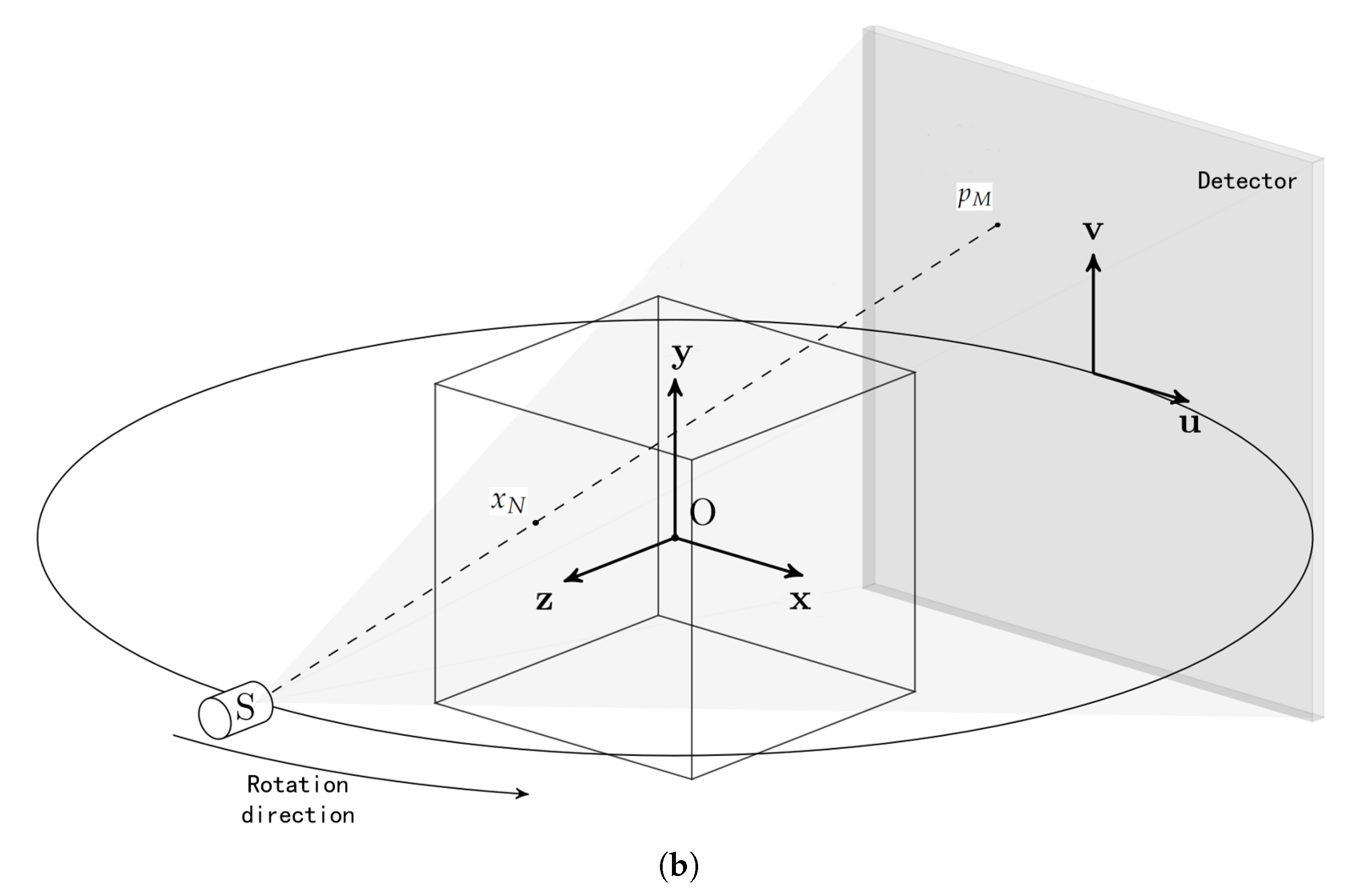
2.1. Reconstruction Model

Assume that $\mathbf{x}={\left[x_1,x_2,\dots ,x_N\right]}^T$ is a one-dimensional vectorization representation of three-dimensional voxels, and $\mathbf{p}={\left[p_1,p_2,\dots ,p_M\right]}^T$ is a one-dimensional vectorization representation of sparse-view projections. The CBCT reconstruction model can be expressed as:

$$\mathbf{p}=\mathbf{Ax}$$

(1)

where $\mathbf{A}$ is a $M\times N$ system matrix, and the i-th element $a_{m,n}$ represents the contribution of the n-th voxel $x_n$ to the m-th projection $p_m$. The element can be scaled by the length of the intersection of the n-th projection ray (that generates $p_m$) with $x_n$. The geometry of a CBCT system is a three-dimensional coordinate system that includes the source position, isocenter (rotation axis), and detector, as shown in Figure 1. The system operates by keeping the X-ray source and detector stationary while the turntable rotates around the y-axis. The geometry description is based on international standard IEC 61217 [21], designed for cone-beam imagers in isocentric radiotherapy systems.

The objective of CBCT reconstruction is to recover the non-negative voxels $\mathbf{x}$ from the projections $\mathbf{p}$ with the known system matrix $\mathbf{A}$. To reduce the radiation dose, sparse projection views are utilized, resulting in insufficient observations and difficulty solving for the voxels from Equation (1). Regularization terms are typically employed to provide additional constraints to the voxels, allowing them to be estimated by solving the following optimization problem:

$$\underset{x}{argmin}{∥\mathbf{Ax}-\mathbf{p}∥}_2^2+\alpha {∥\mathbf{x}∥}_{TV}+\gamma \left(\mathbf{Rx}\right)$$

(2)

where the first term ensures that the projections of the estimated voxels are consistent with the projections captured by the CBCT device, ${∥\mathbf{x}∥}_{TV}$ is the total variation regularization term based on the prior knowledge of the gradient sparsity of the CT reconstruction models, and $R\left(x\right)$ is the denoise regularization term that derives from inherent characteristics of voxel data to provide additional constraints to $\mathbf{x}$. The parameters $\alpha ,\gamma$ are factors to balance the weights of the three terms.

The total variation term ${∥\mathbf{x}∥}_{TV}$ is defined as the sum of the 2-norms of the directional gradients of the variable, it can be described as:

$$\begin{array}{cc}\hfill {∥\mathbf{x}∥}_{TV}=& \sum \sqrt{{(x_{i,j,k}-x_{i-1,j,k})}^2+{(x_{i,j,k}-x_{i,j-1,k})}^2+{(x_{i,j,k}-x_{i,j,k-1})}^2},\hfill \\ \hfill & [i=(1,2,\dots ,I),j=(1,2,\dots ,J),k=(1,2,\dots ,K\left)\right]\hfill \end{array}$$

(3)

where $x_{i,j,k}$ is the number of voxels $\mathbf{x}$ to be reconstructed $\left[(i-1)\times J\times K+(j-1)\times K+k\right]$ elements (I is the length of the voxels, J is the width of the voxels, and K is the height of the voxels, $N=I\times J\times K$).

2.2. Solution Method

To solve Equation (2), the half-quadratic splitting technique is employed to balance the TV term and the denoise term. By introducing an auxiliary variable $\mathbf{f}$ and replacing the variable $\mathbf{x}$ in the denoise term, Equation (2) can be rewritten as:

$$\underset{x}{argmin}{∥\mathbf{Ax}-\mathbf{p}∥}_2^2+\alpha {∥\mathbf{x}∥}_{TV}+\beta {∥\mathbf{f}-\mathbf{x}∥}_2^2+\gamma \mathbf{R}\left(\mathbf{f}\right)$$

(4)

where $\beta$ is the same as $\alpha ,\gamma$. The CBCT reconstruction model defined in Equation (2) is transformed into the alternating iterative optimization of two sub-problems by fixing one variable and solving another alternatively.

$${\mathbf{f}}_{iter+1}=\underset{f}{argmin}\beta {∥\mathbf{f}-{\mathbf{x}}_{iter}∥}_2^2+\gamma \mathbf{R}\left(\mathbf{f}\right)$$

(5)

$${\mathbf{x}}_{iter+1}=\underset{x}{argmin}{∥{\mathbf{Ax}}_{iter}-\mathbf{p}∥}_2^2+\alpha {∥{\mathbf{x}}_{iter}∥}_{TV}+\beta {∥{\mathbf{f}}_{iter+1}-{\mathbf{x}}_{iter}∥}_2^2$$

(6)

2.3. Denoising Image Fusion Algorithm

The original weighted Schatten p-norm minimization (WSNM) algorithm [17] is designed for 2D image denoising. However, the 3D structure information between slices cannot be used for reconstruction by the original WSNM. The WSNM needs to be extended based on 3D block grouping. By referring to the BM3D algorithm and literature [20], we propose a denoising image fusion algorithm for denoising 3D voxel images. The algorithm can be divided into three main steps:

• The 3D noisy voxel $\mathbf{x}$ is divided into three groups of slices according to the direction of the Cartesian coordinate axis: $\left\{X_s^{axis}|axis=x,y,z;s=i,j,k\right\}$.
• Each 2D pure matrix F could be denoised independent through WSNM algorithm from noisy matrix X.
• Fuse $F_s$ by $F_s^x,F_s^y,F_s^z$.

2.3.1. Weighted Schatten p-Norm Minimization Algorithm

The noisy matrix X can be written as $X=F+D$, where D denotes the noise matrix. Due to the similarity of the grouped blocks, the true matrix F is low rank. With the WSNM, the true matrix F is recovered from the noisy matrix X by solving

$$\underset{F}{argmin}\left|\right|X-{F\left|\right|}_F^2+{\left(\sum _{l=1}^L{\omega }_l{\delta }_l^C\right)}^{\frac{1}{C}}$$

(7)

where L is the rank of F, C is the power of Schatten p-norm, ${\omega }_l$ is the l-th singular value of F, and $\omega$ is a weight vector composed of the non-negative weights ${\omega }_l$. The penalty factors $\gamma$ and $\beta$ in Equation (5) are merged into the weight vector $\omega$. It balances the F-norm fidelity term and the Schatten p-norm regularization term.

Assuming ${\sigma }^2$ as the variance of the noisy matrix X, ${\sigma }_l$ is the l-th singular values of the noisy matrix X. X could be decomposed as $X=U\Sigma V$ through SVD and $\Sigma$ is the diagonal matrix of singular values ${\sigma }_l$. By literature [17], Equation (7) could be computed by $F=U\Delta V^T$, where $\Delta =Diag[{\delta }_1,{\delta }_2,\dots ,{\delta }_l,\dots ,{\delta }_L]$ is the diagonal matrix of singular values F. Furthermore, the $\Delta$ could be decoupled into L independent single-variable optimizations without any constraints [17].

$$\begin{array}{c}\hfill \underset{\left\{{\delta }_l\right\}}{argmin}\sum _{l=1}^L[{({\delta }_l-{\sigma }_l)}^2+{\omega }_l{\delta }_l^C]⟺\underset{{\delta }_l}{argmin}{({\delta }_l-{\sigma }_l)}^2+{\omega }_l{\delta }_l^C\end{array}$$

(8)

where ${\delta }_l$ is singular values of F, it obeys ${\delta }_l\ge 0$ and ${\delta }_l\ge {\delta }_{l+1}$. Furthermore, it is solved by using the GST algorithm [19]

$$\left\{\begin{array}{cc}{\delta }_l=0,\hfill & \hfill if{\sigma }_l\le {\left(2{\omega }_l(1-C)\right)}^{\frac{1}{2-C}}+{\omega }_{l}C{\left(\left(2{\omega }_l(1-C)\right)\right)}^{\frac{C-1}{2-C}}\\ {\delta }_l-{\sigma }_l+{\omega }_{l}C{\delta }_l^{C-1}=0,\hfill & \hfill otherwise.\end{array}\right.$$

(9)

The weights $\omega$ in Equation (8) is proportional to the variance of the noise ${\sigma }^2$ which is estimated effectively with the filter-based approaches from the noisy matrix X. Assuming that ${\omega }_l\le {\omega }_{l+1}$, and the true matrix F is unknown, its singular values ${\delta }_l$ are estimated by the singular values $\widehat{{\delta }_l}$ of the noisy matrix X. So, the weights ${\omega }_l$ could be computed by Equation (10):

$$\left\{\begin{array}{cc}\hfill {\omega }_l& =\frac{c\sqrt{S}{\sigma }^2}{{\widehat{\delta }}_l^{\frac{1}{C}}+\epsilon }\hfill \\ \hfill \widehat{{\delta }_l}& =\sqrt{max\{{\sigma }_l^2-S{\sigma }^2,0\}}\hfill \end{array}\right.$$

(10)

where c is a constant and is set to $2\sqrt{2}$, $S=N\times N$ is the number of voxels contained in X, and $\epsilon$ is a minimum value close to zero. Finally, the X is denoised and we get the F. Additionally, the WSNM can work well for most of the noise and artifacts that increased the weighted Schatten p-norm of the data matrix.

2.3.2. Fuse Denosing Image

To obtain the final voxel value $F_{i,j,k}$ from $F_s^x,F_s^y,F_s^z$, we use similarity as the weight criterion for image fusion. It is assumed that the higher the similarity between the denoised slice and the original slice, the worse the denoised effect, that is, the lower the weight. By traversing the three slices corresponding to voxel $F_{i,j,k}$, their similarity is calculated and normalized to obtain the final weight value. Similar to the approach in the literature [22], the similarity coefficient d is defined as follows, and the final voxel value $F_{i,j,k}$ is computed by:

$$\left\{\begin{array}{c}{F}_{i,j,z}=\sum _{a=x,y,z}{\overline{d}}_{i,j,k}^a{F}_{i,j,k}^a\hfill \\ d_{i,j,k}^a(P_a,P_o)=1-\frac{\left|\right|P_a-P_o{\left|\right|}_2^2}{N\times N}\hfill \end{array}\right.$$

(11)

where $\overline{d}$ is the normalized value of similarity coefficient d, $P_a$ is the denoised slice, and $P_o$ is the original slice.

2.4. Adaptive Steepest Descent Projection onto Convex Sets Algorithm

The second sub-problem involves an unconstrained minimization method. In order to solve the sparse problem, the ASD-POCS algorithm is proposed as a robust solution. This algorithm not only minimizes the data constraint with TV regularization but also adaptively controls the TV minimization update to adjust its strength according to the data constraint update. Several adaptations and improvements of this algorithm have been proposed in the literature [23,24,25], all based on the same mathematical approach.

Equation (6) could be written as:

$$\left\{\begin{array}{cc}\hfill {\mathbf{x}}_{iter+1}& =\underset{x}{argmin}{∥{\mathbf{A}}^{\prime }{\mathbf{x}}_{iter}-{\mathbf{p}}^{\prime }∥}_2^2+\alpha {∥{\mathbf{x}}_{iter}∥}_{TV}\hfill \\ \hfill {\mathbf{A}}^{\prime }& =\left(\genfrac{}{}{0pt}{}{\mathbf{A}}{\sqrt{\beta }\mathbf{I}}\right),{\mathbf{p}}^{\prime }=\left(\genfrac{}{}{0pt}{}{\mathbf{p}}{\sqrt{\beta }{\mathbf{f}}_{iter+1}}\right).\hfill \end{array}\right.$$

(12)

By satisfying the Karush–Kuhn–Tucker conditions, the Lagrangian for the Equation (12) could also be defined as:

$$\mathbf{L}=\alpha {∥\mathbf{x}∥}_{TV}+{∥\mathbf{A}{}^{\prime }\mathbf{x}-\mathbf{p}{}^{\prime }∥}_2^2-\lambda \mathbf{x}$$

(13)

So, we can make the gradient of the Lagrangian zero to obtain $\mathbf{x}$, that is, $▽\mathbf{L}=\mathbf{0}$. The Lagrangian form of Equation (13) meets the expression form of ASD-POCS algorithm, and the algorithm in reference [26] can solve $\mathbf{x}$.

The proposed sparse CBCT reconstruction method is summarized in Algorithm 1.

Algorithm 1 CBCT sparse reconstruction based on ADS-POCS and image fusion.

Input:

System matrix $\mathbf{A}$, projection data $\mathbf{p}$;

the power of Schatten p-norm C, the maximum iterative step $Iter$;

the constant C, the minimum value $\epsilon$;

the factors $\alpha$ and $\beta$;

the iteration error ${\epsilon }_{Iter}$;

1:   Standardization of the projection data by literature [22];

2:   If iter = 0, the initial reconstruction $x_0$ by using the FDK algorithm;

3:   iter = 1;

4:   While($iter\ne Iteror\left|\right|x_{iter}-x_{iter-1}{\left|\right|}_2^2\le {\epsilon }_{Iter}$)

5:      divide x into three groups of slices $X_s^{axis}$;

6:      For axis = x,y,z

7:         Singular value decomposition: $X=U\sum V^T$;

8:         Estimate weight vector $\omega$ by using Equation (10);

9:         Calculate $\Delta$ from Equation (8);

10:       Calculate $F^{axis}=U\Delta V^T$;

11:    End

12:    Fuse denoised slice matrix $F^{axis}$ to form $f_{iter+1}$;

13:    calculating $x_{iter+1}$ by using Equation (12)

14:    $iter=iter+1$

15:  End

16:  return $\mathbf{x}$

Output:

Reconstruction voxels $\mathbf{x}$;

3. Results and Discussion

3.1. Experimental Setup

The proposed CBCT reconstruction method was applied to three distinct experiment: a digital brain phantom, a set of real CT data of human lung obtained from the Cancer Imaging Archive (TCIA) [21], and a set of scanned walnut data acquired using a portable CBCT system at our institute.

For the first experiment, the digital brain phantom was utilized. The source-to-detector distance was set at 1536 mm, the source-to-rotation center distance was 1000 mm, and the digital brain phantom size was $512\times 512\times 521$ voxels. The voxel pixel size was 0.5 mm, the detection pixel size was 0.8 mm, and the size of each projection was $512\times 512$ voxels.

Due to the limited availability of CBCT model datasets online, the majority of which are spiral scanning CT data, this study simulates the forward projection process of CBCT by employing publicly available CT datasets to obtain projection data. Compared to experiment 1, experiment 2 utilizes clinical medical data that are more realistic and complex. The results of experiment 2 are more reliable and applicable to practical engineering. The correctness and superiority of the proposed method are verified by applying the proposed method to reconstruct the model and comparing it with the source model and other algorithms. The simulation process for the dataset involves setting the source-to-detector distance at 1536 mm, the source-to-rotation center distance at 1000 mm, the real CT size at $512\times 512\times 241$ voxels, the voxel pixel size at 0.5 mm, the detection pixel size at 0.8 mm, and the size of each projection at $512\times 512$ pixels.

For the third experiment, the source-to-detector distance was set to 952 mm, the source-to-rotation center distance was 593 mm, the detection pixel size was 0.139 mm, and the size of each projection was $1440\times 240$ voxels. The number of projections was 720, with a uniformly spaced angle increment. The detector employed was a Mars 1717V, and the X-ray source was a CANON D-045S. The detailed parameters are as follows:

• X-ray parameters:

  -

  Maximum X-ray tube voltage is 70;

  -

  Focus is 0.4 mm;

  -

  kV The anode (or cathode) indirectly is 35 kV;

  -

  Minimum X-ray tube voltage is 50;

  -

  kV Maximum X-ray tube current of 12;

  -

  mA Maximum filament current is 3.0 A.

• Detector parameters:

  -

  Types of detectors is amorphous silicon;

  -

  Type of scintillator is CsI;

  -

  Effective imaging area (inch) is $17\times 17$;

  -

  Pixel size ($\mathsf{\mu }$m) is 139;

  -

  Spatial resolution (lp/mm) is 3.6;

  -

  AD converted bits (bit) is 16;

  -

  Dimensions (mm${}^3$) is $460\times 460\times 15$;

  -

  Weight (kg) is 4.6;

  -

  Power dissipation (W) is Max.20.

The reconstruction experiments were conducted using the Python 3.8.12 programming environment, leveraging the Tomographic Iterative GPU-based Reconstruction Toolbox (TIGRE) open-source software for reconstruction and 3D Slicer for visualization. The code was executed on a personal computer running Windows 10 with an Intel^® Core™ i9-10900K CPU @ 3.70 GHz and 32 GB memory. Element-wise computation of the transform and adjoint transform was accelerated by an NVIDIA^® GeForce RTX™ 3080 graphics processor. Three standard metrics were employed to quantitatively assess the proposed method: RMSE, SSIM, and PSNR.

RMSE is commonly used to evaluate the differences between two signals and is defined as:

$$RMSE(x,x^{*})=\sqrt{\frac{1}{N}\sum _{i=1}^N{(x-x^{*})}^2}$$

(14)

where x is the reconstructed result, $x^{*}$ is the ground truth, and N is the total number of voxels. The PSNR is defined as:

$$PSNR(x,x^{*})=10lo{g}_{10}\frac{{(2^l-1)}^2}{RMSE}$$

(15)

where l is the number of bits for the signal. The SSIM measures the structural similarity of two signal, which is defined as:

$$SSIM(x,x^{*})=\frac{2{\mu }_x{\mu }_{x^{*}}(2{\sigma }_{x{x}^{*}}+c_2)}{({\mu }_x^2+{\mu }_{x^{*}}^2+c_1)({\sigma }_x^2+{\sigma }_{x^{*}}^2+c_2)}$$

(16)

where ${\mu }_x$ and ${\mu }_{x^{*}}$ denote the mean values of x and $x^{*}$, respectively, ${\sigma }_x$ and ${\sigma }_{x^{*}}$ represent the standard deviations, and ${\sigma }_{x{x}^{*}}$ is the covariance. $c1$ and $c2$ are constants to avoid instability, which are set to $0.0001{(2^l-1)}^2$ and $0.0009{(2^l-1)}^2$, respectively.

3.2. Sparse Reconstruction of Digital Brain Phantom

The digital brain phantom, widely employed for evaluating CBCT reconstruction, was used for validation. We sampled 90 projection images using the forward method through the TIGRE Toolkit and added noise with a level of $Poisson={10}^5,Gaussian=[0,10]$. The original digital brain slice served as a benchmark for CBCT reconstruction. Additionally, four classical methods discussed in the introduction—FDK, OS-SART, ASD-POCS, and ordered subset ASD-POCS (OS-ASD-POCS)—were used for comparison.

Reconstruction results are displayed in Figure 2, with the 160th slice in the sagittal (Y-axis) direction chosen for comparison due to its information richness. FDK, proposed for full-view reconstruction, produces an acceptable image from sufficient projection data but suffers from severe streak artifacts in Figure 2b when projection data are insufficient. Streak artifacts are still apparent in Figure 2c for OS-SART but are significantly reduced compared to FDK. Edges appear blurred and some critical structural details are lost in Figure 2d,e, despite ASD-POCS’s ability to remove artifacts and suppress noise. For a clearer comparison, the region of interest (ROI) marked by the red box in Figure 2d,e is magnified and displayed in Figure 3. The noise reduction effect of the proposed method outperforms that of the ASD-POCS and OS-ASD-POC algorithms.

Figure 4 illustrates voxel curves and their local magnifications along the coronal axis (256th row, 160th slice) and the vertical axis (256th column, 160th slice). As depicted in Figure 4b,c, the proposed method performs substantially better than FDK and OS-SART for smooth segments, which have curves heavily disturbed by noise. As seen in Figure 4e,f, the proposed method outshines ASD-POCS and OS-ASD-POCS for steep segments, with curves significantly affected by noise.

Concurrently, evaluation results are provided in

Table 1. Quantitative evaluation for brain phantom reconstruction from 90 views.

	RMSE	PSNR	SSIM
FDK	0.01482	18.29061	0.70205
OS-SART	0.00069	31.61237	0.93187
ASD-POCS	0.00006	42.01851	0.98943
OS-ASD-POCS	0.00032	35.00853	0.96763
Proposed Method	0.00008	44.54638	0.98968

using RMSE, PSNR, and SSIM. From the perspectives of PSNR and SSIM, the proposed method and the ASD-POCS method exhibit high structural similarity and signal-to-noise ratio. Regarding RMSE, the proposed method is slightly higher than ASD-PCOS, potentially due to the addition of WSNM noise reduction, increasing the error from the ground value. Considering all three indicators, the proposed method excels in terms of signal-to-noise ratio and structural similarity, with a minor disadvantage in RMSE but a small difference.

3.3. Sparse Reconstruction of Downloaded CBCT Projections

The digital CT model dataset was obtained from [27]. We extracted 45 projections from the dataset with a resolution of $512\times 512$, as shown in Figure 5. This model serves as a benchmark for CBCT reconstruction. In addition to FDK, OS-SART, ASD-POCS, and OS-ASD-POCS, comparisons were made.

Reconstruction results are presented in Figure 6, with the 121st slice in the axial direction chosen for comparison due to its information richness. The CT model slice is shown in Figure 6a. Similarly to Experiment 1, Figure 6b reveals that FDK and OS-SART algorithms exhibit relatively severe streak artifacts, while ASD-POCS and OS-ASD-POCS suppress artifacts but blur the edges. From the reconstruction results, it is evident that the proposed method outperforms the other algorithms in

Table 2. Quantitative evaluation for walnut reconstruction from 45 views.

	RMSE	PSNR	SSIM	Time Consumption (Second)
FDK	0.14376	8.42370	0.68207	514.73
OS-SART	0.14018	8.53299	0.58307	30,420.12
ASD-POCS	0.14020	8.53264	0.68359	376,080.45
OS-ASD-POCS	0.14020	8.53257	0.58362	57,120.36
Proposed Method	0.14420	8.56196	0.70640	58,648.75

.

Upon comparing reconstruction times, it was determined that in Experiment 2, the FDK algorithm had the shortest processing time for clinical projection data, while the iterative ASD-POCS algorithm had the longest processing time. By improving the ordered subset method, processing time can be effectively reduced. Although the proposed algorithm has a longer processing time compared to the OS-ASD-POCS algorithm, its reconstruction results exhibit higher PSNR and SSIM values. This is due to the addition of a denoising process in this algorithm. Overall, the proposed algorithm strikes an optimal balance between processing time and reconstruction results.

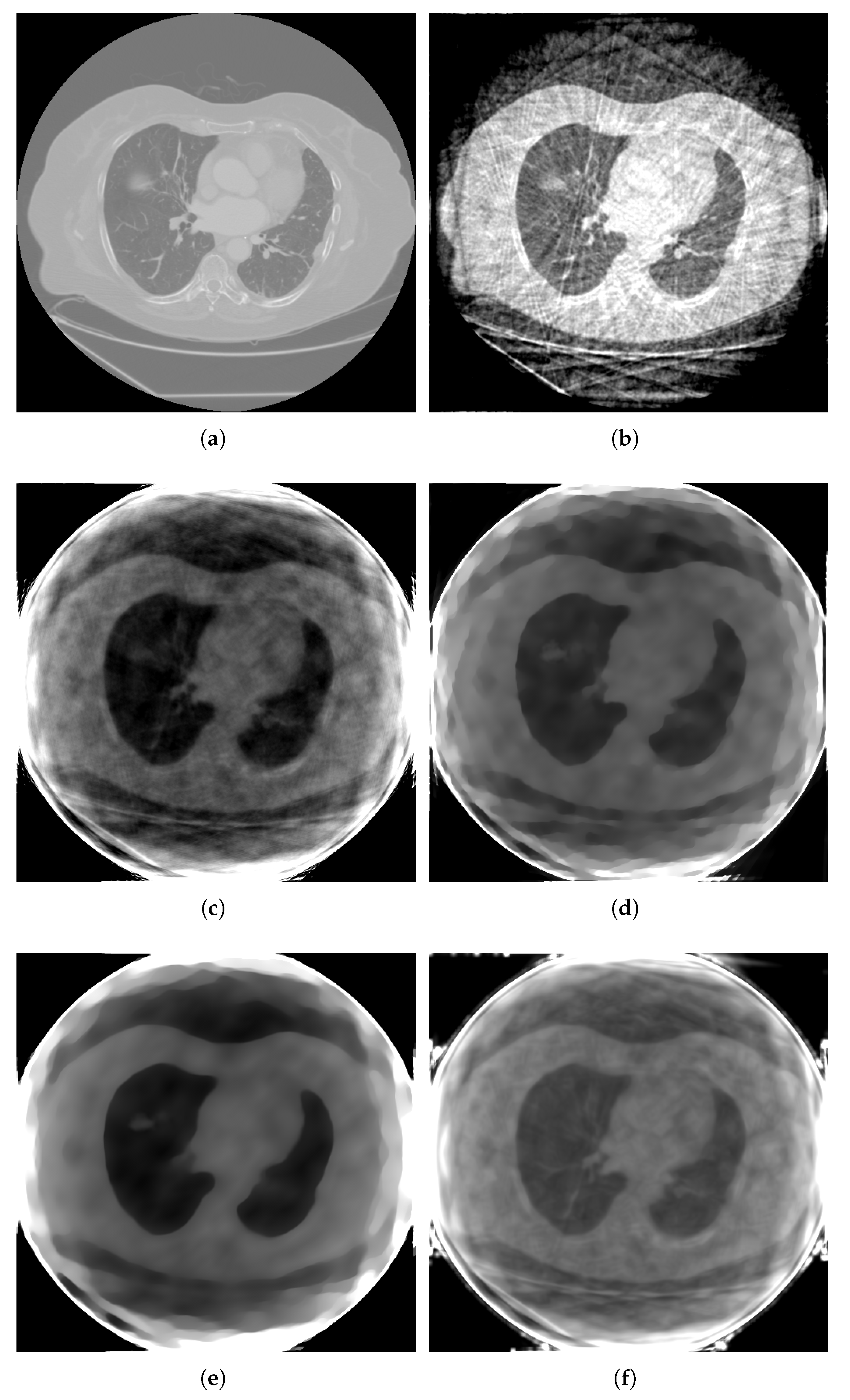
3.4. Sparse Reconstruction of Real Projections

The CBCT projections of a real walnut were obtained from our laboratory. We sampled 60 projection images from 720 projections at moderate intervals for reconstruction, maintaining a size of $512\times 512$ pixels, as shown in Figure 7. Projections were reconstructed using FDK, ASD-POCS, and the proposed method. FDK for full sampling of 720 projections was used as a benchmark for CBCT reconstruction.

Reconstruction results are displayed in Figure 8, where the 256th slice in the sagittal (Y-axis) direction is selected for comparison due to its information richness. FDK for full-view reconstruction constructs an acceptable image from sufficient projection data in Figure 8a. However, it is severely marred by streak artifacts in Figure 8b when projection data are insufficient. The walnut slice is displayed in Figure 8a. As observed in Experiment 3, Figure 8c,d shows that sharp edges are blurred, and some critical structural details are lost, even though ASD-POCS and OS-ASD-POCS can suppress artifacts and blur edges. In contrast, the proposed method effectively removes artifacts and suppresses noise.

4. Conclusions

In this paper, we propose a novel iterative algorithm for sparse-view CBCT reconstruction, aiming to correct artifacts and reduce noise. The method consists of two primary steps: ADS-POCS reconstruction and denoising, which can be solved iteratively. The image fusion algorithm based on WSNM effectively utilizes 3D voxel information to reduce noise, while other artifacts are addressed by the ADS-POCS algorithm that incorporates TV regularization. The proposed method is validated using a digital head phantom and clinical data. Performance is measured using RMSE, PSNR, and SSIM, demonstrating the algorithm’s ability to effectively remove artifacts and suppress noise. Furthermore, we employ a self-developed portable CBCT device for reconstruction and compare the results with those of other algorithms. Although the proposed method outperforms the alternatives, there are some bright areas observed on sharp edges, attributable to the balance adjustment issue between noise reduction and artifact removal. Future work will address this issue.

Moving forward, it is essential to consider reconstruction challenges arising from more complex low-dose factors such as limited angles and reduced mAs (the product of tube current and exposure time) levels. Simultaneously, enhancing the computational speed of the reconstruction and minimizing the time required for reconstruction are critical for practical engineering applications.

References

1. Wang, Y.; Yang, T.; Huang, W. Limited-angle computed tomography reconstruction using combined FDK-based neural network and U-Net. In Proceedings of the 2020 42nd Annual International Conference of the IEEE Engineering in Medicine & Biology Society (EMBC), Montreal, QC, Canada, 20–24 July 2020; pp. 1572–1575. [Google Scholar]
2. Rathore, J.S.; Laquai, R.; Biguri, A.; Soleimani, M.; Vienne, C. Benchmarking of different reconstruction algorithms for industrial cone-beam CT. In Proceedings of the 11th Conference on Industrial Computed Tomography, Wels, Austria (ICT 2022), Wels, Austria, 8–11 February 2022; pp. 1–8. [Google Scholar]
3. Zhou, B.; Chen, X.; Zhou, S.K.; Duncan, J.S.; Liu, C. DuDoDR-Net: Dual-domain data consistent recurrent network for simultaneous sparse view and metal artifact reduction in computed tomography. Med. Image Anal. 2022, 75, 102289. [Google Scholar] [CrossRef] [PubMed]
4. Jerri, A.J. The Shannon sampling theorem—Its various extensions and applications: A tutorial review. Proc. IEEE 1977, 65, 1565–1596. [Google Scholar] [CrossRef]
5. Donoho, D.L. Compressed sensing. IEEE Trans. Inf. Theory 2006, 52, 1289–1306. [Google Scholar] [CrossRef]
6. Candes, E.J. The restricted isometry property and its implications for compressed sensing. C. R. Math. 2008, 346, 589–592. [Google Scholar] [CrossRef]
7. Sidky, E.Y.; Pan, X. Image reconstruction in circular cone-beam computed tomography by constrained, total-variation minimization. Phys. Med. Biol. 2008, 53, 4777. [Google Scholar] [CrossRef] [PubMed]
8. Yang, F.; Zhang, D.; Zhang, H.; Huang, K.; Du, Y.; Teng, M. Streaking artifacts suppression for cone-beam computed tomography with the residual learning in neural network. Neurocomputing 2020, 378, 65–78. [Google Scholar] [CrossRef]
9. Sori, W.J.; Feng, J.; Godana, A.W.; Liu, S.; Gelmecha, D.J. DFD-Net: Lung cancer detection from denoised CT scan image using deep learning. Front. Comput. Sci. 2021, 15, 152701. [Google Scholar] [CrossRef]
10. Wang, T.; Xia, W.; Huang, Y.; Sun, H.; Liu, Y.; Chen, H.; Zhou, J.; Zhang, Y. DAN-Net: Dual-domain adaptive-scaling non-local network for CT metal artifact reduction. Phys. Med. Biol. 2021, 66, 155009. [Google Scholar] [CrossRef]
11. Croton, L.C.; Ruben, G.; Morgan, K.S.; Paganin, D.M.; Kitchen, M.J. Ring artifact suppression in X-ray computed tomography using a simple, pixel-wise response correction. Opt. Express 2019, 27, 14231–14245. [Google Scholar] [CrossRef]
12. Mäkinen, Y.; Azzari, L.; Foi, A. Collaborative filtering of correlated noise: Exact transform-domain variance for improved shrinkage and patch matching. IEEE Trans. Image Process. 2020, 29, 8339–8354. [Google Scholar] [CrossRef] [PubMed]
13. Dabov, K.; Foi, A.; Katkovnik, V.; Egiazarian, K. Image restoration by sparse 3D transform-domain collaborative filtering. In Proceedings of the Image Processing: Algorithms and Systems VI; SPIE: Bellingham, WA, USA, 2008; Volume 6812, pp. 62–73. [Google Scholar]
14. Mäkinen, Y.; Marchesini, S.; Foi, A. Ring artifact and Poisson noise attenuation via volumetric multiscale nonlocal collaborative filtering of spatially correlated noise. J. Synchrotron Radiat. 2022, 29, 829–842. [Google Scholar] [CrossRef] [PubMed]
15. Dong, W.; Li, Z.; Xiang, D. Prior image constrained low-rank matrix decomposition method in limited-angle reverse helical cone-beam CT. J. X-ray Sci. Technol. 2015, 23, 759–772. [Google Scholar] [CrossRef] [PubMed]
16. Gu, S.; Xie, Q.; Meng, D.; Zuo, W.; Feng, X.; Zhang, L. Weighted nuclear norm minimization and its applications to low level vision. Int. J. Comput. Vis. 2017, 121, 183–208. [Google Scholar] [CrossRef]
17. Xie, Y.; Gu, S.; Liu, Y.; Zuo, W.; Zhang, W.; Zhang, L. Weighted Schatten p-norm minimization for image denoising and background subtraction. IEEE Trans. Image Process 2016, 25, 4842–4857. [Google Scholar] [CrossRef]
18. Xu, J.; Cheng, Y.; Ma, Y. Weighted schatten p-norm low rank error constraint for image denoising. Entropy 2021, 23, 158. [Google Scholar] [CrossRef] [PubMed]
19. Zuo, W.; Meng, D.; Zhang, L.; Feng, X.; Zhang, D. A generalized iterated shrinkage algorithm for non-convex sparse coding. In Proceedings of the IEEE International Conference on Computer Vision, Sydney, Australia, 1–8 December 2013; pp. 217–224. [Google Scholar]
20. Xu, C.; Yang, B.; Guo, F.; Zheng, W.; Poignet, P. Sparse-view CBCT reconstruction via weighted Schatten p-norm minimization. Opt. Express 2020, 28, 35469–35482. [Google Scholar] [CrossRef] [PubMed]
21. IEC. IEC 61217:2011. Available online: https://webstore.iec.ch/publication/4929 (accessed on 7 December 2011).
22. Zhang, J.; He, B.; Yang, Z.; Kang, W. A Novel Geometric Parameter Self-Calibration Method for Portable CBCT Systems. Electronics 2023, 12, 720. [Google Scholar] [CrossRef]
23. Liu, L.; Yin, Z.; Ma, X. Nonparametric optimization of constrained total variation for tomography reconstruction. Comput. Biol. Med. 2013, 43, 2163–2176. [Google Scholar] [CrossRef] [PubMed]
24. Liu, Y.; Ma, J.; Fan, Y.; Liang, Z. Adaptive-weighted total variation minimization for sparse data toward low-dose x-ray computed tomography image reconstruction. Phys. Med. Biol. 2012, 57, 7923. [Google Scholar] [CrossRef] [PubMed]
25. Tian, Z.; Jia, X.; Yuan, K.; Pan, T.; Jiang, S.B. Low-dose CT reconstruction via edge-preserving total variation regularization. Phys. Med. Biol. 2011, 56, 5949. [Google Scholar] [CrossRef] [PubMed]
26. Biguri, A. Iterative Reconstruction and Motion Compensation in Computed Tomography on GPUs. Ph.D. Thesis, University of Bath, Bath, UK, 2018. [Google Scholar]
27. TICA. The Cancer Imaging Archive. Available online: http://www.cancerimagingarchive.net (accessed on 20 December 2016).
Figure 1. The components of portable CBCT system: (a) 3D real view; (b) spatial geometry.
Mathematics 11 02127 g001aMathematics 11 02127 g001b
Figure 2. Brain phantom reconstruction (slice 160): (a) ground truth, (b) FDK, (c) OS-SART, (d) ASD-POCS, (e) OS-ASD-POCS, (f) proposed method.
Mathematics 11 02127 g002
Figure 3. Zoom in on ROI in Figure 2: (a) ASD-POCS, (b) OS-ASD-POC, (c) proposed method.
Mathematics 11 02127 g003
Figure 4. Voxel curves reconstructed by various algorithms: (a) voxel curve along coronal axis at 256th row, 160th slice, (b,c) local magnifications of (a); (d) voxel curve along axial axis at 256th column, 160th slice; (e,f) local magnifications of (d).
Mathematics 11 02127 g004
Figure 5. CT Model: (a) Model in three-dimensional view; (bd) Slices of the model in the axial, coronal, and sagittal planes, respectively.
Mathematics 11 02127 g005
Figure 6. The CT reconstruction (slice 121): (a) CT model, (b) FDK, (c) OS-SART, (d) ASD-POCS, (e) OS-ASD-POCS, (f) proposed method.
Mathematics 11 02127 g006
Figure 7. Walnut projections at different angle: (a) projection at 0 rotation; (b) projection at 90 rotation; (c) projection at 180 rotation.
Mathematics 11 02127 g007
Figure 8. The walnut reconstruction (slice at 256 sagittal axis): (a) FDK reconstructed by 720 projections, (b) FDK, (c) ASD-POCS, (d) proposed method.
Mathematics 11 02127 g008