Article

Improved Beluga Whale Optimization for Solving the Simulation Optimization Problems with Stochastic Constraints

by
Shih-Cheng Horng
1,* and
Shieh-Shing Lin
2
1
Department of Computer Science & Information Engineering, Chaoyang University of Technology, Taichung 413310, Taiwan
2
Department of Electrical Engineering, St. John’s University, New Taipei City 251303, Taiwan
*
Author to whom correspondence should be addressed.
Mathematics 2023, 11(8), 1854; https://doi.org/10.3390/math11081854
Submission received: 21 March 2023 / Revised: 11 April 2023 / Accepted: 11 April 2023 / Published: 13 April 2023
(This article belongs to the Special Issue Nature Inspired Computing and Optimisation)

Abstract

:
Simulation optimization problems with stochastic constraints are optimization problems with deterministic cost functions subject to stochastic constraints. Solving the considered problem by traditional optimization approaches is time-consuming if the search space is large. In this work, an approach integration of beluga whale optimization and ordinal optimization is presented to resolve the considered problem in a relatively short time frame. The proposed approach is composed of three levels: emulator, diversification, and intensification. Firstly, the polynomial chaos expansion is treated as an emulator to evaluate a design. Secondly, the improved beluga whale optimization is proposed to seek N candidates from the whole search space. Eventually, the advanced optimal computational effort allocation is adopted to determine a superior design from the N candidates. The proposed approach is utilized to seek the optimal number of service providers for minimizing staffing costs while delivering a specific level of care in emergency department healthcare. A practical example of an emergency department with six cases is used to verify the proposed approach. The CPU time consumes less than one minute for six cases, which demonstrates that the proposed approach can meet the requirement of real-time application. In addition, the proposed approach is compared to five heuristic methods. Empirical tests indicate the efficiency and robustness of the proposed approach.

1. Introduction

Simulation optimization problems with stochastic constraints (SOPSC) are optimization problems that optimize a deterministic cost function subject to stochastic constraints on the variables [1]. Such problems become more and more popular over the years in many practical applications, such as dynamic production/inventory lot-sizing problems, power transmission grid reliability problems, signaling-regulatory pathway inference problems, and staffing optimization of emergency department healthcare. The SOPSC belong to the class NP-hard, and their suboptimal designs are usually difficult to solve in a reasonable time [2,3].
The SOPSC are difficult to solve because of the three challenges, (i) a large search space, (ii) ensuring that all constraints are met, and (iii) accurately estimating a stochastic constraint is time-consuming. The ordinal optimization (OO) theory [4,5] has emerged as an efficient technique to handle issues (i) to (iii) simultaneously. Instead of insisting on picking the best design, OO theory focuses on seeking good enough designs and decreases the simulation time significantly. OO theory can seek good enough solutions with high probability through relatively short simulations. The OO theory attempts to resolve the difficulties by employing the following two ideas. (i) The order of a design is more resilient against noise than the value of a design. (ii) Since seeking the best design is computationally expensive, it would be wiser to concentrate on good enough designs. The OO theory has been applied successfully to many situations, including routing optimization in queueing networks [6], staff optimization in multi-skill call centers [7], job-shop scheduling [8], and optimization of shortcuts in the sorting conveyor system [9].
Although the OO theory can expedite the search process by quickly narrowing down the search space, the stochastic constraints still significantly influence the computing efficiency. To decrease the computational time of SOPSC, an algorithm that integrates beluga whale optimization and ordinal optimization (BWOO) is presented to seek a superior design within a short time frame. The BWOO comprises three phases: emulator, diversification, and intensification. First of all, the polynomial chaos expansion (PCE) [10,11] is treated as an emulator to evaluate a design. Secondly, an improved beluga whale optimization (IBWO) is proposed to seek N candidates from the whole search space. Then, an advanced optimal computational effort allocation (AOCBA) is adopted to determine a superior design from the N candidates. These three phases significantly decrease the computing time to solve the SOPSC.
Instead of handling an approximated mathematical model, the optimal staffing cost in emergency department healthcare can be modeled as a SOPSC. Next, the BWOO is utilized to seek the number of staff for minimizing staffing costs while delivering a specific level of care. The target of this SOPSC is to determine the optimal number of service providers to minimize staffing costs while delivering a specific level of care. The contribution of the paper is twofold. First, we develop a BWOO algorithm to seek a superior design of a SOPSC which is short of structural information in a relatively short period. Second, the BWOO algorithm is utilized to determine the optimal staffing cost in emergency department healthcare. The application of the BWOO algorithm is not confined to the SOPSC. The proposed approach can also be utilized to solve computationally expensive simulation optimization problems, discrete probabilistic bicriteria optimization problems, probabilistic constrained simulation optimization problems, and combinatorial stochastic simulation optimization problems.
The remainder of the paper develops as follows. Section 2 introduces the related works of SOPSC. Section 3 illustrates the BWOO algorithm to seek a superior design of a SOPSC. Section 4 introduces the optimal staffing cost in emergency department healthcare, which can be modeled as a SOPSC. Then, the BWOO algorithm is utilized to solve this SOPSC. Section 5 is the comparative analysis of the experimental verification. Finally, the conclusion and further research are presented in Section 6.

2. Literature Review

Popular approaches which are frequently employed to solve SOPSC include the sample path approach, stochastic approximation, and sample average approximation. The sample path approach approximates the output through the average sample observations using a common sequence of random numbers. The stochastic approximation approach approximates the output in an environment where the output is unknown and direct observations are corrupted by noise [12]. The sample average approximation approach uses an approximation scheme by sample averages and replication over several iterations [13]. However, slow convergence rate and trapping in local minima are two drawbacks of the three approaches.
Heuristic algorithms are existing techniques used to solve SOPSC, including tabu search (TS) [14], simulated annealing (SA) [15], genetic algorithm (GA) [16], particle swarm optimization (PSO) [17], differential evolution (DE) [18], biogeography-based optimization (BBO) [19], and social network optimization (SNO) [20]. However, heuristics methods lack the power and flexibility to create ongoing optimal designs. Swarm intelligence (SI) algorithms have fast developed in recent years and applied to solve SOPSC [21]. SI algorithms are inspired by swarms that frequently occur in the real world such as bird flocks, fish schools, and the colony of social insects. The recent novel SI algorithms include golden jackal optimization (GJO) [22], starling murmuration optimizer (SMO) [23], white shark optimizer (WSO) [24], dandelion optimizer (DO) [25], search in forest optimizer (SIFO) [26], snake optimizer (SO) [27], and beluga whale optimization (BWO) [28]. SI algorithms are proven to perform better than conventional optimization approaches and are widely applied in many fields.
BWO is a revolutionary nature-inspired scheme that simulates the attacking and feeding behaviors of beluga whales in nature [28]. The BWO has obvious advantages such as better stability, stronger search ability, higher convergence accuracy, and faster convergence speed. However, BWO has a lack of diversity, which could lead to being trapped in local optimum and premature convergence. To overcome this drawback, the proposed IBWO is developed to accelerate the search process, improve the learning approach, and increase the variety and strengthen the consistency of the chosen candidates.
The optimal staffing costs in the emergency department healthcare can be formulated as a SOPSC. Over the years, common solution approaches for solving the optimal number of staff include the greedy approach, exhaustive search, branch, and bound method, approximate dynamic programming method, and heuristic algorithms [29]. The greedy approach employs the problem-solving heuristic of selecting the design that is optimal locally at each stage in the pursuit of the global optimum [30]. An exhaustive search is simply a brute-force approach to the considered problem. The branch and bound scheme partitions the feasible design space into smaller subsets of designs. However, it is necessary to search all the design spaces if the worst-case occurs. The approximate dynamic programming technique has a complicated design process, which results in a long computing time [31]. Recently, heuristic algorithms are faster and provide near-optimal designs. However, heuristic algorithms still get stuck in being premature and always fall into the local optimum. An intelligent inventory model is proposed to find the optimal service strategy based on the variable conditions along with the optimal quantity and reorder level of the inventory policy [32]. Table 1 shows the research gaps and contributions of the previous author(s).

3. Integrating Beluga Whale Optimization and Ordinal Optimization

3.1. Mathematical Formulation

The SOPSC has the following two challenges, (i) the search space often lacks structural information to identify the optimal design, and (ii) because of the randomness of the constraints, the feasibility of a design cannot certainly be known. The SOPSC are typically shown below.
min h ( x )
subject   to   E [ g i ( x ) ] d i , i = 1 , , I
Y x U
where x = [ x 1 , , x J ] T depicts a design vector, h ( x ) denotes the deterministic cost function, E [ g i ( x ) ] depicts the expectation of the ith constrained function, d i depicts pre-specified requirement values, I depicts the number of constraints, Y = [ Y 1 , , Y J ] T and U = [ U 1 , , U J ] T denote the lower and upper bounds, respectively.
Sufficient replications must be executed to achieve an exact evaluation of E [ g i ( x ) ] . However, executing an infinitely long simulation is impossible. Therefore, the following sample mean is an alternative formula to estimate E [ g i ( x ) ] .
g ¯ i ( x ) = 1 L = 1 L g i ( x ) , i = 1 , , I
where L depicts the amount of replications, and g i ( x ) represents the estimation of the th replication. When the number of replications increases, the sample mean g ¯ i ( x ) will have a preferable estimation of E [ g i ( x ) ] . That is, a larger value of L is more closely approximate E [ g i ( x ) ] .
Since the constraints are usually soft ones, the SOPSC is imposed by adding an extra penalty [33]. An infeasible design is penalized so that its chance of survival is much decreased as compared to a feasible design.
min f ( x ) = h ( x ) + η × i = 1 I p e i ( x )
where η depicts a penalty factor, f(x) depicts a penalized cost function, and p e i ( x ) represents the quadratic penalty function.
p e i ( x ) = { 0 , i f g ¯ i ( x ) d i , ( g ¯ i ( x ) d i ) 2 ,   else , i = 1 , , I .
The penalty factor is usually a positive constant that is large enough to enlarge the penalty function whenever a constraint is violated. Let L a represent the sufficient large value of L , and the exact evaluation of (4) is calculated using L = L a . For simplicity, we let   f a ( x ) indicate the penalized cost function of x through exact evaluation.
The OO theory [4] elaborates that orders of designs are still retained even though they are evaluated by a crude model. Therefore, the PCE emulator is utilized to estimate a design more quickly. Thus, the IBWO cooperated with the PCE emulator is employed to look for N candidates from the whole search space.

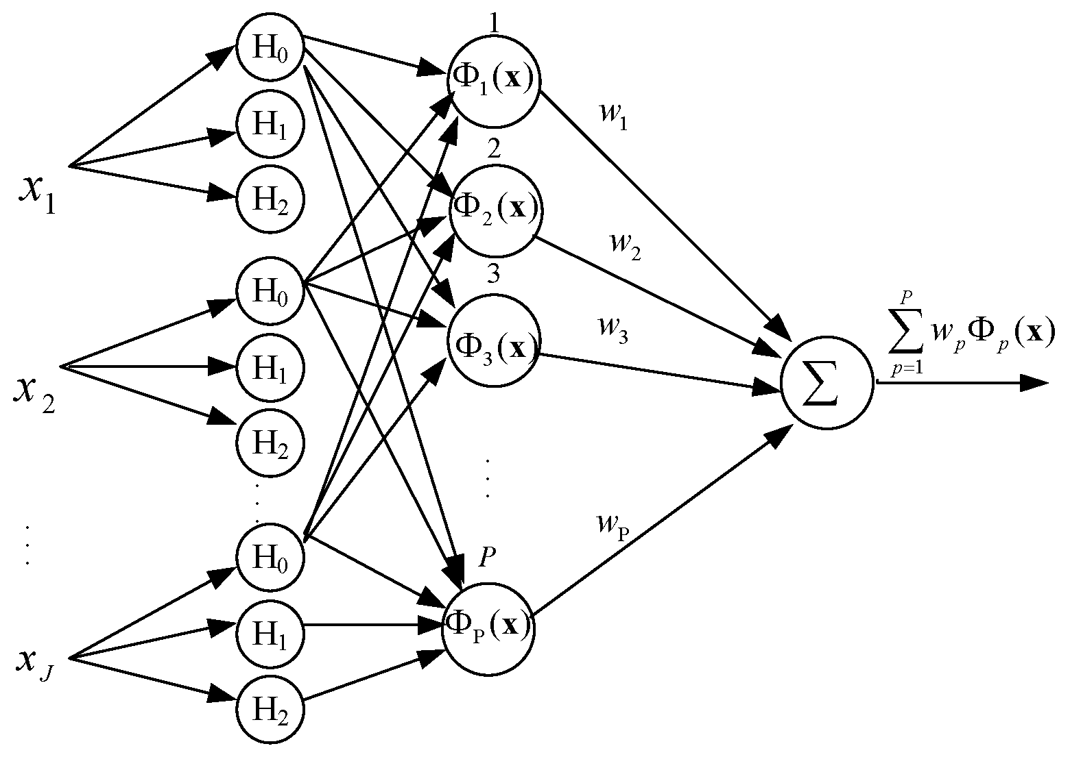
3.2. Polynomial Chaos Expansion

The emulator is an important and growing field of research that signifies a major achievement in surrogate modeling, including the support vector regression [34], multivariate adaptive regression splines [35], extreme learning machines [36], regularized minimal-energy tensor-product splines [37], and polynomial chaos expansions (PCE) [10,11]. Among them, PCE builds a polynomial approximation of a model whose inputs are random variables. There are three advantages of PCE: (i) it allows for uncertainty quantification of input parameters, (ii) it can be evaluated much faster than the stochastic response itself, and (iii) its exact analytical expression. PCE has been widely adopted in various applications, including curve fitting, forecasting, prediction, and function approximation [10]. Therefore, the PCE emulator is used to quickly evaluate a design. The PCE with second-order chaos polynomial factor is composed of three layers as shown in Figure 1.
The PCE utilizes orthogonal polynomials as a basis for the fitting of response outputs based on a probabilistic data set. We randomly sample Π   x ’s from search space and evaluate   F a ( x ^ ) using exact evaluation, where x ^ = x μ σ are the normal standard of x , and µ and σ represent the mean and standard deviation, respectively. We represent these Π sampled designs as ( x ^ i ,   F a ( x ^ i ) ). The PCE can approximate F ( x ^ ) using sums of orthonormal polynomials.
F ( x ^ ) = p = 1 P w p Φ p ( x ^ )
where P denotes the quantity of PCE terms; w p are the expansion coefficients; and Φ p ( x ^ ) are multivariate orthogonal polynomial basis functions, which are built as a product of univariate polynomials as follows.
Φ p ( x ^ ) = k = 1 K H p ( x ^ k )
where K is the dimension of a multivariate orthogonal polynomial, which is obtained by the input data through the Hermite polynomials H p ( ) . These data points of Φ p ( x ^ ) can be extracted from the input variables in the modeling process through the Hermite polynomials. For example, if P = 2, H 0 ( x ^ ) = 1 , H 1 ( x ^ ) = x ^ , and H 2 ( x ^ ) = x ^ 2 1 . The least-square-minimization method is used to determine the expansion coefficients w p , p = 1 , , P .
[ w 1 w P ] = [ Φ T Φ ] 1 Φ T [ F a ( x ^ 1 ) F a ( x ^ Π ) ]
The setting of Π must be larger than the setting of P, i.e., Π > P. The matrix Φ is determined as follows.
Φ = [ Φ 1 ( x ^ 1 ) Φ 2 ( x ^ 1 ) Φ P ( x ^ 1 ) Φ 1 ( x ^ Π ) Φ 2 ( x ^ Π ) Φ P ( x ^ Π ) ]
The PCE is trained offline to significantly decrease the computing burden. After training the PCE, the model can be generalized with a new design x to predict F ( x ^ ) .

3.3. Improved Beluga Whale Optimization

In the diversification phase, we can adapt state-of-the-art optimization techniques with the assistance of the PCE to look for N candidates from the whole search space. Since the BWO explores several regions at the same time, it is more suitable for the specific requirements. In essence, BWO uses the following three behaviors: pair swim, prey, and whale fall. The pair swims behavior is corresponding to exploration. Beluga whales engage in social interactions under different postures, such as two beluga whales swimming in close pairs in a synchronized or mirrored manner. The preying behavior is corresponding to exploitation. Beluga whales cooperatively feed and move based on the location of nearby companions. Beluga whales prey by sharing each other’s location information, considering the top candidates and others. Exploration is related to global search as well as exploitation is related to local search. In the first one, we are interested in exploring the search space looking for good solutions, whereas, in the second one, we want to refine the solution and try to avoid big jumps in the search space. The whale fall is corresponding to imitating small changes in the groups. During the migration and foraging, some beluga whales do not survive and fall into the depths of the ocean.
The proposed IBWO has three algorithmic parameters, including a balance factor between exploration and exploitation (Bf), the probability of whale fall (Wf), and the jump strength of Levy flight (Cf). BWO has a lack of diversity, which could lead to being trapped in local optimum and premature convergence. To overcome these drawbacks, the three algorithmic parameters Bf, Wf, and Cf are iteratively modified to intensify exploration in the former process and exploitation in the latter process. The variation of Bf decreases exponentially with increased iterations. A large Bf focuses on finding promising regions at the beginning, then a small Bf focuses on searching near already found promising designs near the end. The variation of Wf and Cf are also exponentially decreased as iterations increase to strengthen exploitation.
The following notations are used in IBWO. Ψ depicts the number of beluga whales, t max denotes the maximum number of iterations, x i t = [ x i , 1 t , , x i , J t ] T and r i t = [ r i , 1 t , , r i , J t ] T are the positions of the ith beluga whale and a randomly selected beluga whale at iteration t, respectively, and x * = [ x 1 * , , x J * ] T is the position of the elite beluga whale. B f t [ B f _ min , B f _ max ] , W f t [ W f _ min , W f _ max ] , and C f t [ C f _ min , C f _ max ] depict the balance factor Bf, probability Wf, and jump strength Cf at iteration t, respectively, where B f _ min , W f _ min , C f _ min are lower bound, and B f _ max , W f _ max , C f _ max are upper bound.
The details of the IBWO algorithm are explained as follows (Algorithm 1).
Algorithm 1: The IBWO
Step 1: Configuration of parameters
Set parameters to Ψ , B f _ min , B f _ max , W f _ min , W f _ max , C f _ min , C f _ max , and t max . Create an index variable t and initialize it to 0.
Step 2: Initialize the population
Initialization of a population with Ψ beluga whales.
x i 0 = Y + r a n d [ 0 , 1 ] × ( U Y ) ,   i = 1 , , Ψ .
where r a n d [ 0 , 1 ] is a random number in the range 0 to 1, and Y and U represent the lower and upper bounds, respectively.
Step 3: Ranking
(a)
Compute f ( x i t ) of every beluga whale cooperated with PCE, i = 1 , , Ψ .
(b)
Sort the Ψ beluga whales on the basis of their fitness from the least to the biggest, then determine the elite x * .

Step 4: Modify three algorithmic parameters
B f t = B f _ min + ( B f _ max B f _ min ) × exp ( ln ( B f _ min B f _ max ) × t t max )
W f t = W   f _ m a x × exp ( W   f _ m a x W f _ m i n × t t m a x )
C f t = C f _ min + ( C f _ max C f _ min ) × ( 1 exp ( C f _ max C f _ min × ( t t max 1 ) ) )

Step 5: Exploration and exploitation
If B f t > 0.5 , perform exploration.
x i , j t + 1 = { x i , p t + ( x r , q t x i , p t ) × ( 1 + r a n d [ 0 , 1 ] ) × sin ( 2 π r a n d [ 0 , 1 ] ) , j = e v e n x i , p t + ( x r , q t x i , p t ) × ( 1 + r a n d [ 0 , 1 ] ) × cos ( 2 π r a n d [ 0 , 1 ] ) , j = o d d , i = 1 , , Ψ
where r is an arbitrarily chosen beluga whale, p and q are random numbers selected from J-dimension, when x i , j t + 1 < Y j , set x i , j t + 1 = Y j , and when x i , j t + 1 > U j , set x i , j t + 1 = U j .
Else if B f t 0.5 , perform exploitation.
x i t + 1 = r a n d [ 0 , 1 ] x * r a n d [ 0 , 1 ] x i t + C   f t L F ( x r t x i t ) , i = 1 , , Ψ .
where r is an arbitrarily chosen beluga whale, x * is the elite beluga whale, C   f t denotes the jump strength of Levy flight, and LF denotes the following Levy flight function,
L F = 0 . 05   × u | v | 1 β ×   ( Γ ( 1 + β ) × sin ( π β / 2 ) Γ ( ( 1 + β ) / 2 ) × β × 2 β - 1 2 ) 1 β
where u and v indicate the mean and standard derivation in Gauss distribution with u = 0, Γ denotes the Gamma function, and β = 1.5 is a default value. When x i , j t + 1 < Y j , set x i , j t + 1 = Y j , and when x i , j t + 1 > U j , set x i , j t + 1 = U j .
Step 6: Whale fall
If B f t W f t ,
x i t + 1 = r a n d [ 0 , 1 ] x i t r a n d [ 0 , 1 ] x r t + r a n d [ 0 , 1 ] ( U V ) e 2 Ψ W f t × t t max , i = 1 , , Ψ .
where r is a randomly selected beluga whale. When x i , j t + 1 < Y j , set x i , j t + 1 = Y j , and when x i , j t + 1 > U j , set x i , j t + 1 = U j .
Step 7: Replace elitism
Compute F ( x i t + 1 ) and F ( x * ) cooperated with PCE and adopt the greedy approach between x i t + 1 and x * . If F ( x i t + 1 ) < F ( x * ) , set x * = x i t + 1 .
Step 8: Termination
If t t max , terminate; else, set t = t + 1 and return to Step 2.
The IBWO stops after the t max iterations have been executed. When the IBWO is suspended, the Ψ beluga whales are ordered on the basis of their fitness. Although the IBWO is designed for continuous variables, a real value can be rounded to the nearest integer through the bracket function z i , j t max = x i , j t max , where x i , j t max and z i , j t max Z . Then, the prior N beluga whales are chosen to constitute the candidate subset.

3.4. Advanced Optimal Computing Budget Allocation

To increase the computing efficiency of the original OCBA, the AOCBA is utilized to determine a superior design from the candidate subset. The AOCBA allocates the computational effort sequentially to all the competing alternatives based on the means and variances. In the original OCBA, all replications must be performed at every iteration to calculate the statistics of competing alternatives. The AOCBA just needs to carry out incremental replications every iteration to calculate the statistics of competing alternatives. In the AOCBA, more computing budget is allocated to simulating critical alternatives, and less is allocated to non-critical alternatives. Emphasizing little critical alternatives not only saves computational effort but also reduces the variances of critical alternatives. AOCBA is developed to improve the computing efficiency of OO by distributing the computational effort reasonably. OO theory allocates identical computational effort to every competing alternative, while AOCBA allocates computational effort to a competing alternative based on its performance. Thus, AOCBA proposes a way of asymptotically optimal allocation of computing budget among competing alternatives.
The number of incremental replications can be allocated to critical designs through the statistics obtained from the N candidates. Let C a represent the available computational effort, L 0 indicate the essential replications allocated to each candidate, and L n denote the replications assigned to the n th candidate. A one-time incremental computational effort, Δ, is provided in every iteration. Typically, the best setting of Δ is problem-dependent and can be found by experimentation. A large setting of Δ results in a waste of computational effort to accomplish an unnecessarily high confidence level, while a small setting of Δ performs the allocating procedure many times. The AOCBA aims at maximizing the probability of correct selection given that L 1 + L 2 + + L N = C a by intelligently allocating C a to L 1 ,…, ,…, L N . The available computational budget C a is defined as C a = N × L a τ , where L a is the replications adopted in the exact evaluation, and τ depicts a speed-up factor [38,39] (Algorithm 2).
Algorithm 2: The AOCBA
Step 1. Define the values of L 0 , set l = 0 , L n l = L 0 , n = 1 , , N , and calculate the available computational effort C a = N × L a τ .
Step 2. Add a one-time incremental computing budget Δ to n = 1 N L n l , and update the replications.
L j l + 1 = ( n = 1 N L n l + Δ ) × θ j l / ( θ b l + n = 1 , n b N θ n l )
L b l + 1 = θ b l θ j l × L j l + 1
L n l + 1 = θ n l θ j l × L j l + 1
where θ n l θ j l = ( δ n l × ( f ¯ b l f ¯ j l ) δ j l × ( f ¯ b l f ¯ n l ) ) 2 , θ b l = δ b l n = 1 , n b N ( θ n l δ n l ) 2 , f ¯ n l = 1 L n l k = 1 L n l f k ( x n ) , δ n l = 1 L n l h = 1 L n l ( f k ( x n ) f ¯ n l ) 2 for all n j b , b = arg min n f ¯ n l , x n represents the nth candidate, and f k ( x n ) denotes the penalized objective value of x n at the kth replication.
Step 3. Perform incremental replications of max [ 0 , L n l + 1 L n l ] to the nth candidate, and calculate the incremental mean ( f ^ n l + 1 ) and incremental standard deviation ( δ ^ n l + 1 ).
f ^ n l + 1 = 1 ( L n l + 1 L n l ) k = L n l + 1 L n l + 1 f k ( x n )
δ ^ n l + 1 = 1 ( L n l + 1 L n l ) k = L n l + 1 L n l + 1 (   f k ( x n ) f ^ n l + 1 ) 2

Step 4. Compute the updated mean ( f ¯ n l + 1 ) and updated standard deviation ( δ   n l + 1 ) of the n th candidate for overall replications.
f ¯ n l + 1 = 1 L n l + 1 ( L n l × f ¯ n l + ( L n l + 1 L n l ) × f ^ n l + 1 )
δ n l + 1 = 1 ( L n l + 1 1 ) × ( L n l ( f ¯ n l ) 2 + ( L n l 1 ) ( δ n l ) 2 + ( L n l + 1 L n l ) ( f ^ n l + 1 ) 2 + ( L n l + 1 L n l 1 ) ( δ ^ n l + 1 ) 2 L n l + 1 ( f ^ n l + 1 ) 2 )
Step 5. If n = 1 N L n l C a , stop and determine the optimal x * with the minimum objective value; else, let l = l + 1 and go to Step 1.

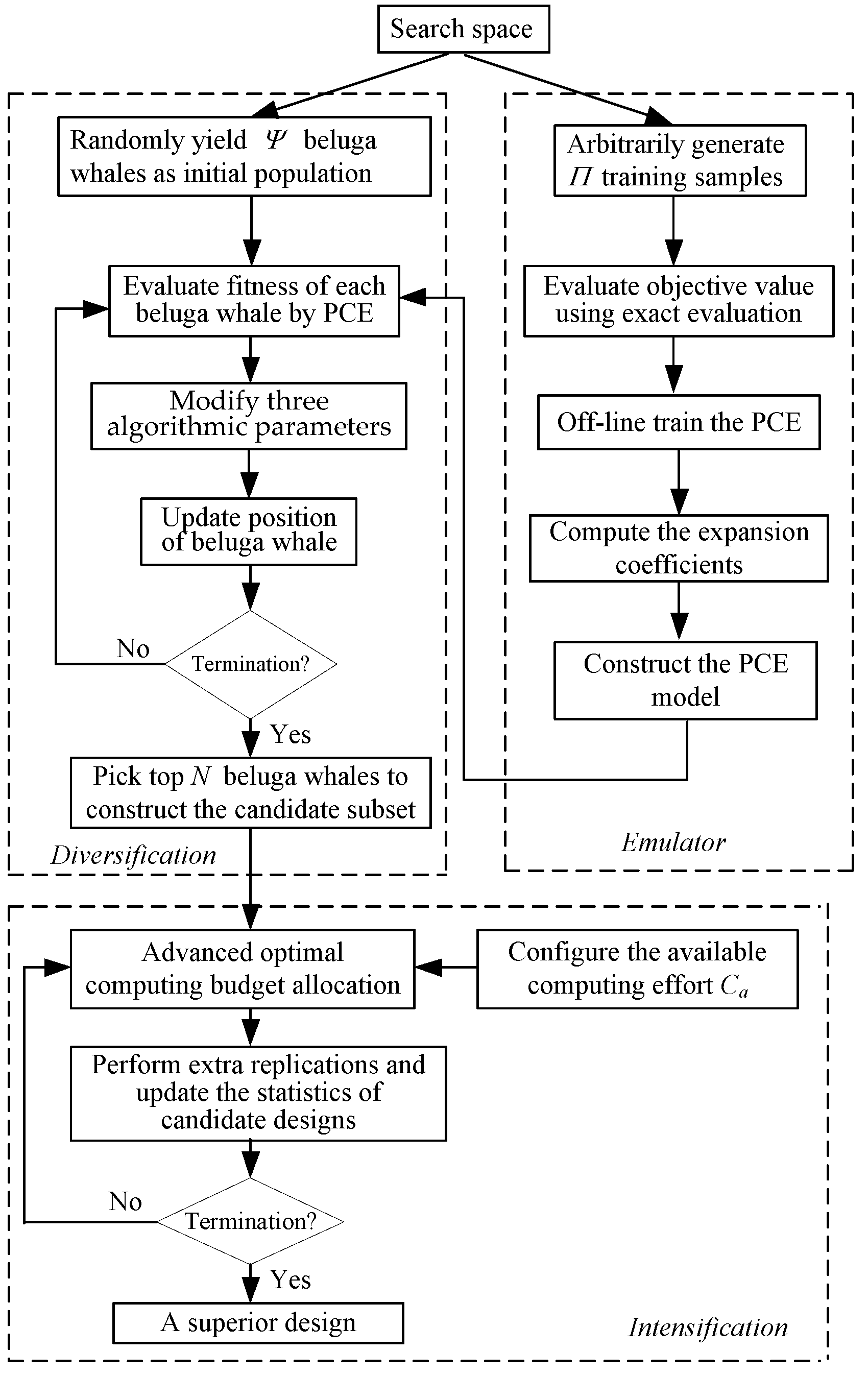
3.5. The BWOO Algorithm

The flowchart of the BWOO algorithm (Algorithm 3) is presented in Figure 2.
Algorithm 3: The BWOO
Step 1: Define the values of Ψ , B f _ min , B f _ max , W f _ min , W f _ max , C f _ min , C f _ max , t max , N , L a , L 0 , and Δ .
Step 2: Randomly select Π x ’s from the search space, evaluate f a ( x ) using exact evaluation, and train the PCE offline using these Π designs.
Step 3: Generate Ψ x ’s to be the initial population, then apply the IBWO algorithm to those beluga whales that cooperated with PCE. After the IBWO algorithm terminates, rank all the final Ψ x ’s based on their approximate fitness from the lowest to the highest, and choose the prior N x ’s to construct a candidate subset.
Step 4: Apply the AOCBA algorithm to the N candidates and determine the optimum x * , which is the superior design.

4. Optimal Staffing Cost in the Emergency Department Healthcare

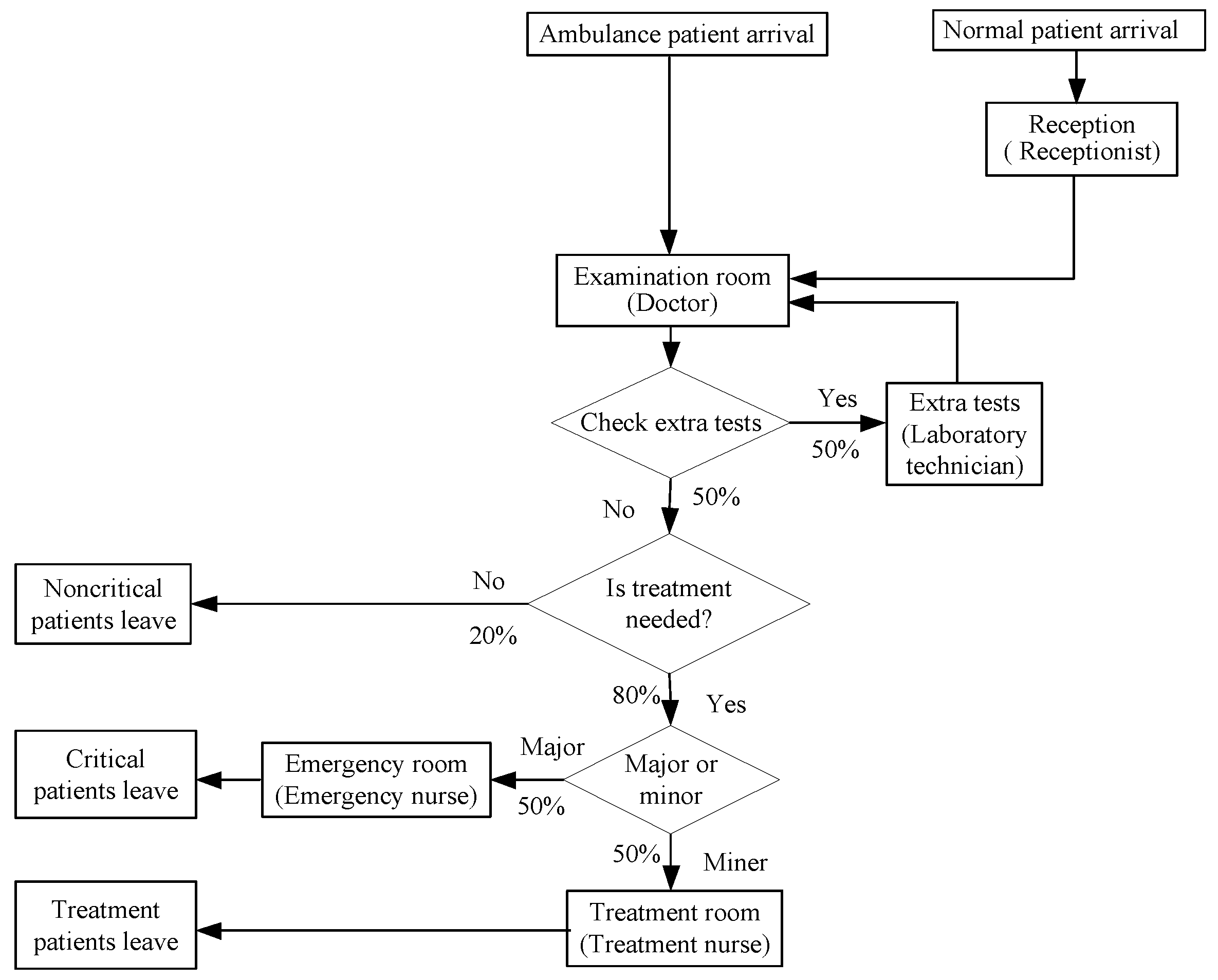
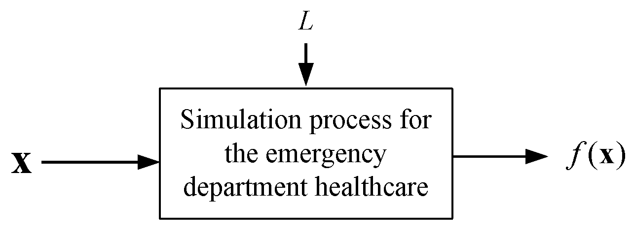
4.1. Emergency Department Healthcare

Most emergency departments have a recognizable patient arrival pattern, which follows a process as depicted in Figure 3. The patient flow process is modeled through a discrete-event simulation modeling with the following five assumptions. (i) The arrival patient to the reception follows a nonstationary Poisson process with a rate of λ(t). (ii) The arrival patient to the examination room follows a Poisson process with a constant rate. (iii) The routing probabilities of various patients are given at each location. (iv) The number of staff at each location decides the allocation of the system. (v) The distribution of service time and the rates are given.
Now, the optimal staffing cost in the emergency department healthcare is formulated as a SOPSC as follows.
min   h ( x )
  subject   to   E [ g 1 ( x ) ] d 1
E [ g 2 ( x ) ] d 2
Y x U
where x = [ x 1 , , x 5 ] T indicates a design, x 1 ~ x 5 depicts the number of receptionists, doctors, laboratory technicians, treatment nurses, and emergency nurses, respectively, E [ g 1 ( x ) ] represents the average waiting time of critical patients, d 1 is prespecified requirement values of critical patients, E [ g 2 ( x ) ] represents the average waiting time of treatment patients, d 2 is prespecified requirement values of treatment patients, h ( x ) is the staffing cost, and Y and U denote the lower and upper bounds, respectively.
The target of the SOPSC is to find the optimal number of staff x * to minimize staffing cost h ( x ) subject to integrality conditions, two constraints, and limits of staff members. The sample mean is one of the most common alternatives to estimate the value of E [ g i ( x ) ] .
g ¯ i ( x ) = 1 L = 1 L g i ( x ) , i = 1 , 2 .
where L represents the quantity of replications, and g i ( x ) is the estimation of the th replication. Since the constraints are soft, the penalty function is employed for handling the two inequality constraints.
min f ( x ) = h ( x ) + η × i = 1 2 p e i ( x )
where η depicts a penalty factor,   f ( x ) is a penalized cost function, and p e i ( x ) denotes the quadratic penalty function.
p e i ( x ) = { 0 , i f   g ¯ i ( x ) d i , ( g ¯ i ( x ) d i ) 2 , else , i = 1 , 2 .
Figure 4 describes the input/output relationship of the emergency department healthcare, where x depicts a design and   f ( x ) depicts the penalized cost function. Let L a indicate the sufficiently large value of L , and the exact evaluation of (31) is defined as L = L a . For simplicity,   f a ( x ) is denoted as the penalized cost function of x obtained by an exact evaluation.

4.2. Application of the BWOO Method

4.2.1. Constitute the Emulator

Four procedures were utilized for constructing the PCE emulator to evaluate a design. (i) Arbitrarily chose Π   x ’s from search space and calculate   f a ( x ) by exact evaluation, then indicate these Π designs and their estimations as x i and f a ( x i ) , respectively. (ii) Set the number of PCE terms, i.e., P = 2. (iii) Pre-compute the matrix of multivariate orthogonal polynomial basis functions. (iv) Compute the expansion coefficients.

4.2.2. Construct the Candidate Subset

With the assistance of the PCE emulator, N candidates were selected by the IBWO. First of all, Ψ beluga whales were randomly generated to be the initial population. The fitness of a beluga whale was calculated using the PCE emulator. When the IBWO stopped after t max iterations, the Ψ beluga whales were sorted based on their fitness. The former N beluga whales were selected to constitute the candidate subset.

4.2.3. Find the Superior Design

Eventually, the AOCBA method was adopted to seek a superior design from the N candidates. In general, the number of N cannot be too large to improve efficiency. On the other hand, some outstanding designs will miss when the setting of N is too small. Reference [38] suggested that a suitable value of L 0 is between 5 to 20, and an appreciate the value of Δ is smaller than 100 but larger than 10% of N.

5. Practical Applications

5.1. Practical Example

A practical example of an emergency department adopted and extended from the stochastic resource problem 3 in [40] is used to verify the BWOO method. Because of operating cost considerations, at most 5 receptionists, 7 doctors, 6 laboratory technicians, 8 treatment nurses, and 10 emergency nurses can be employed. The target is to find how many staff members could be employed to minimize staffing costs while delivering a specific level of care. We assume that receptionists, doctors, laboratory technicians, and both treatment nurses and emergency nurses earn $40, $120, $50, and $30, respectively.
The arrival pattern of walk-in patients follows a nonstationary Poisson process based on Table 2. The arrival pattern of ambulance patients follows a Poisson process with a constant rate of 2 per hour. Distributions of service time at each stage are listed in Table 3. The lower and upper bounds are the two parameters in the parentheses of the uniform distribution. The min, mode, and max are the three parameters in the parentheses of the triangular distribution. We run for 100 more days and adopt a four-day warm-up period. We have conducted six cases of different parameters d1 and d2. Parameters d1 and d2 indicate pre-specified requirements of the average waiting time for critical patients and treatments for patients, respectively. The six cases are obtained by permutations using different values of d1 (2, 2.5, and 3 h) and d2 (2 and 2.5 h).
There are 8549 arbitrarily selected designs to train the PCE. The number of samples Π = 8549 was obtained by the sampling size formula using a confidence interval of 1% and a confidence level of 95% [41]. The performance of a sample was evaluated by an exact evaluation.
The penalty factor was η = 10 4 . A large penalty factor is assured to amplify the penalty function for infeasible designs. The lower and upper bounds were Y = [ 1 , 1 , 1 , 1 , 1 ] T and U = [ 5 , 7 , 6 , 8 , 10 ] T , respectively. Thus, the size of the search space is 77,760. The parameters used in IBWO were B f _ min = 0.5 , B f _ max = 1 , W f _ min = 0.05 , W f _ max = 0.3 , C f _ min = 0.1 , C f _ max = 2 , t max = 100 , and Ψ = 40 . Various hand-tuned experiments demonstrate that IBWO utilizing the above parameters is well-performed. Figure 5 illustrates the curves of three factors Bf, Wf, and Cf over 100 iterations. The IBWO explored the search space in preceding iterations as well as exploited the certain region in later iterations. The number of candidates was N = 10. The parameters used in AOCBA were L 0 =20, Δ =10 and L a = 10 4 . The speed-up factor τ corresponding to N = 10 is 3.4 [38]. Thus, the available computing effort C a was 29,412.
Table 4 presents the superior design x * , cost, and CPU times of six cases. For example, the optimization model in Case IV gives a design that costs $630 and staff assignment as follows: 1 receptionist, 3 doctors, 1 laboratory technician, 3 treatment nurses, and 3 emergency nurses, such that a limited average waiting time for both critical patients and treatment of patients of 2.5 h. Figure 6 displays the convergence curve of the best-so-far candidate solution for Case IV. The CPU time consumes less than one minute for six cases, which demonstrates that the BWOO can meet the requirement of real-time application.

5.2. Performance Comparison

The BWOO algorithm was compared to five metaheuristic methods for case I: GA [14], ant colony optimization (ACO) [42], clonal selection algorithm (CSA) [43], whale optimization algorithm (WOA) [44], and equilibrium optimization (EO) [45]. A population size of 40, roulette wheel selection, single-point crossover with a crossover probability of 0.8, and uniform mutation with a mutation rate of 0.02 were adopted in the GA. In the employed ACO, a population size of 40, an initial pheromone of 0.1, a global pheromone volatile factor of 0.3, the local pheromone evaporation rate of 0.5, the relative importance of information with 1, and the control factor between the relative proportion of the exploitation and biased exploration with 0.9 were utilized. A population size of 40, a strength of mutation of 10, and a receptor editing rate of 0.05 were adopted in the CSA. In the WOA, a population size of 40, and the shape of a logarithmic spiral of 2 were employed. In the EO, a population of particles of 40, a generation rate of 0.5, a diversification factor of 3, and the exploitation factor of 1 were employed.
The exact evaluation was used to calculate the objective value for five metaheuristic methods. Because of randomness, 30 trials were conducted to verify the reliability of six methods. Since the five metaheuristic methods need more computation times to seek the optimum, the search processes terminated after they had spent 30 min of computation time. Table 5 illustrates the statistical results and average CPU times over 30 trials for 6 approaches. The averages of the best-so-far objective value obtained by GA, ACO, CSA, WOA, and EO were 13.16%, 15.79%, 18.42%, 10.53%, and 11.40% larger than that obtained by BWOO, respectively. Experimental results illustrate that the BWOO outperforms five metaheuristic methods.
Finally, an analysis concerning rank percentage was conducted to illustrate the rank of a superior design in the search space. Because it is impossible to decide the ranks of all designs, a representative subset, Ω , is constructed to represent the characteristics of the large search space. The rank percentage of a superior design is defined as r | Ω | × 100 % , where r indicates the rank of a superior design in Ω . Generally, 11,556 designs were arbitrarily chosen from the whole search space to constitute the representative subset. The objective values of all samples were computed using exact evaluation. The value of | Ω | = 11556 was calculated by the sampling size formula with a confidence interval of 1% and a confidence level of 98% [41]. Table 5 also illustrates the average rank percentages resulting from 6 methods. The standard error of the mean (S.E.M.) resulting from BWOO was 2.73. The small S.E.M. illustrates that most of the superior designs resulting from the BWOO are fairly close to the optimum over 30 trials.

6. Conclusions and Outlooks

To solve the SOPSC in a reasonable time, an algorithm integrating BWO into OO was developed. The BWOO composes of three phases: emulator, diversification, and intensification. The PCE emulator was efficient in rapidly evaluating a design. The BWOO adopted the IBWO for diversification and the AOCBA for intensification. The BWOO was adopted for the optimal staffing cost in the emergency department healthcare, which is modeled as a SOPSC. A practical emergency department with six cases was utilized to test the BWOO algorithm. The CPU time consumes less than one minute for six cases, which demonstrates that the BWOO can meet the real-time requirement. The BWOO was compared to five metaheuristic methods—GA, ACO, CSA, WOA, and EO cooperated with an exact evaluation. Test results demonstrated that most of the superior designs resulting from the BWOO are fairly close to the optimum over 30 trials. Since the BWOO usually obtains a near optimum in a reasonable time, the limitation of the proposed method is that it does not provide a globally optimal solution. The PCE emulator can be replaced by the essential replications L 0 adopted in the AOCBA to resolve this limitation. Futures researches will focus on applying OO to resolve stochastic dominance-constrained optimization problems, such as risk-averse stochastic optimization problems and conditional value-at-risk optimization problems.

Author Contributions

S.-C.H. Horng designed and conceived the experiments; S.-C.H. Horng performed the experiments; S.-S.L. Lin analyzed the data; S.-S.L. Lin contributed reagents and analysis tools; S.-C.H. Horng wrote the paper. All authors have read and agreed to the published version of the manuscript.

Funding

This research was supported in part by the National Science and Technology Council in Taiwan, under Grant MOST111-2221-E-324-021.

Institutional Review Board Statement

Not applicable.

Informed Consent Statement

Not applicable.

Data Availability Statement

Not applicable.

Conflicts of Interest

The authors declare no conflict of interest.

Nomenclature

x = [ x 1 , , x J ] T A design vector
h ( x ) Deterministic cost function
E [ g i ( x ) ] The expectations of the ith constrained function
INumber of constraints (unit)
d i Pre-specified requirement values
Y = [ Y 1 , , Y J ] T Lower bound
U = [ U 1 , , U J ] T Upper bound
g ¯ i ( x ) Sample mean
LNumber of replications (unit)
g i ( x ) Estimation of the th replication
η Penalty factor
  f ( x ) Penalized cost function
p e i ( x ) Quadratic penalty function
L a The replications of the exact evaluation (unit)
  f a ( x ) Penalized cost function through an exact evaluation
PThe number of PCE terms (unit)
w p Expansion coefficients
Φ p ( x ^ ) Multivariate orthogonal polynomial basis functions
H p ( ) Hermite polynomials
Π Number of training samples (unit)
Φ Mapping vector of the expansion coefficients
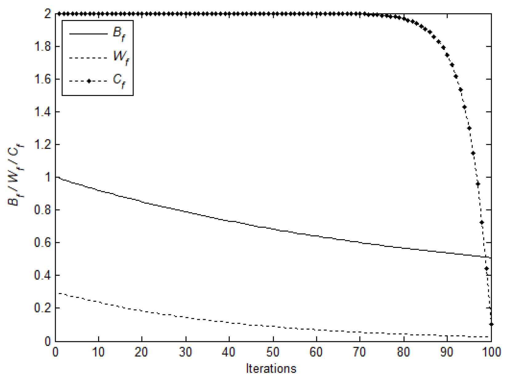
BfBalance factor between exploration and exploitation
WfProbability of whale fall (percentage)
CfJump strength of Levy flight
Ψ Total number of beluga whales (unit)
t max Maximum number of iterations (unit)
x i t = [ x i , 1 t , , x i , J t ] T The position of the ith beluga whale at iteration t
r i t = [ r i , 1 t , , r i , J t ] T The position of a randomly selected beluga whale at iteration t
x * = [ x 1 * , , x J * ] T The position of the elite beluga whale
B f _ min The lower bound of Bf
B f _ max The upper bound of Bf
W f _ min The lower bound of Wf
W f _ max The upper bound of Wf
C f _ min The lower bound of Cf
C f _ max The upper bound of Cf
LFLevy flight function
C a The available computational effort (units)
N Number of candidates (unit)
L 0 The essential replications (units)
L n The replications allocated to the nth candidate (units)
ΔA one-time incremental computational effort
τ A speed-up factor
f ^ n l + 1 Incremental mean
δ ^ n l + 1 Incremental standard deviation
f ¯ n l + 1 Updated mean for overall replications
δ   n l + 1 The updated standard deviation for overall replications
λ ( t ) The arrival interval rate of a patient (1/unit time)
x = [ x 1 , , x 5 ] T A design vector
E [ g 1 ( x ) ] Average waiting time of critical patients (time unit)
E [ g 2 ( x ) ] Average waiting time of treatment patients (time unit)
Π Number of randomly chosen samples (unit)
Ω A representative subset
r The rank of a superior design in Ω

References

  1. Ta, T.A.; Mai, T.; Bastin, F.; L’Ecuyer, P. On a multistage discrete stochastic optimization problem with stochastic constraints and nested sampling. Math. Program. 2021, 190, 1–37. [Google Scholar] [CrossRef]
  2. Lu, X.N.; Peng, Z.L.; Zhang, Q.; Yang, S.L. Event-based optimization approach for solving stochastic decision problems with probabilistic constraint. Optim. Lett. 2021, 15, 569–590. [Google Scholar] [CrossRef]
  3. Latour, A.L.D.; Babaki, B.; Fokkinga, D.; Anastacio, M.H.; Hoos, H.H.; Nijssen, S. Exact stochastic constraint optimisation with applications in network analysis. Artif. Intell. 2022, 304, 103650. [Google Scholar] [CrossRef]
  4. Ho, Y.C.; Zhao, Q.C.; Jia, Q.S. Ordinal Optimization: Soft Optimization for Hard Problems; Springer: New York, NY, USA, 2007. [Google Scholar]
  5. Long, T.; Jia, Q.S.; Wang, G.M.; Yang, Y. Efficient real-time EV charging scheduling via ordinal optimization. IEEE Trans. Smart Grid 2021, 2, 4029–4038. [Google Scholar] [CrossRef]
  6. Horng, S.C.; Lee, C.T. Integration of ordinal optimization with ant lion optimization for solving the computationally expensive simulation optimization problems. Appl. Sci. 2021, 11, 136. [Google Scholar] [CrossRef]
  7. Horng, S.C.; Lin, S.S. Coupling elephant herding with ordinal optimization for solving the stochastic inequality constrained optimization problems. Appl. Sci. 2020, 10, 2075. [Google Scholar] [CrossRef] [Green Version]
  8. Horng, S.C.; Lin, S.S. Ordinal optimization to optimize the job-shop scheduling under uncertain processing times. Arab. J. Sci. Eng. 2022, 47, 9659–9671. [Google Scholar] [CrossRef]
  9. Horng, S.C.; Lin, S.S. Incorporate seagull optimization into ordinal optimization for solving the constrained binary simulation optimization problems. J. Supercomput. 2023, 79, 5730–5758. [Google Scholar] [CrossRef]
  10. Liu, Y.; Zhao, G.; Li, G.; He, W.X.; Zhong, C.T. Analytical robust design optimization based on a hybrid surrogate model by combining polynomial chaos expansion and Gaussian kernel. Struct. Multidiscip. Optim. 2022, 65, 335. [Google Scholar] [CrossRef]
  11. Yao, W.; Zheng, X.H.; Zhang, J.; Wang, N.G.; Tang, G.J. Deep adaptive arbitrary polynomial chaos expansion: A mini-data-driven semi-supervised method for uncertainty quantification. Reliab. Eng. Syst. Saf. 2023, 229, 108813. [Google Scholar] [CrossRef]
  12. Geiersbach, C.; Loayza-Romero, E.; Welker, K. Stochastic approximation for optimization in shape spaces. SIAM J. Optim. 2021, 31, 348–376. [Google Scholar] [CrossRef]
  13. Zhou, X.J.; Wang, X.Y.; Huang, T.W.; Yang, C.H. Hybrid intelligence assisted sample average approximation method for chance constrained dynamic optimization. IEEE Trans. Industr. Inform. 2021, 17, 6409–6418. [Google Scholar] [CrossRef]
  14. Yu, C.L.; Lahrichi, N.; Matta, A. Optimal budget allocation policy for tabu search in stochastic simulation optimization. Comput. Oper. Res. 2023, 150, 106046. [Google Scholar] [CrossRef]
  15. Cheng, D.L. Water allocation optimization and environmental planning with simulated annealing algorithms. Math. Probl. Eng. 2022, 2022, 2281856. [Google Scholar] [CrossRef]
  16. Zhang, Q.B.; Yang, S.X.; Liu, M.; Liu, J.X.; Jiang, L. A new crossover mechanism for genetic algorithms for Steiner tree optimization. IEEE Trans. Cybern. 2022, 52, 3147–3158. [Google Scholar] [CrossRef]
  17. Xu, H.Q.; Gu, S.; Fan, Y.C.; Li, X.S.; Zhao, Y.F.; Zhao, J.; Wang, J.J. A strategy learning framework for particle swarm optimization algorithm. Inf. Sci. 2023, 619, 126–152. [Google Scholar] [CrossRef]
  18. Wang, Y.; Liu, Z.; Wang, G.G. Improved differential evolution using two-stage mutation strategy for multimodal multi-objective optimization. Swarm Evol. Comput. 2023, 78, 101232. [Google Scholar] [CrossRef]
  19. Daneshyar, S.A.; Charkari, N.M. Biogeography based optimization method for robust visual object tracking. Appl. Soft Comput. 2022, 122, 108802. [Google Scholar] [CrossRef]
  20. Beccaria, M.; Niccolai, A.; Zich, R.E.; Pirinoli, P. Shaped-beam reflectarray design by means of social network optimization (SNO). Electronics 2021, 10, 744. [Google Scholar] [CrossRef]
  21. Tang, J.; Liu, G.; Pan, Q.T. A review on representative swarm intelligence algorithms for solving optimization problems: Applications and trends. IEEE/CAA J. Autom. Sin. 2021, 8, 1627–1643. [Google Scholar] [CrossRef]
  22. Chopraa, N.; Ansarib, M.M. Golden jackal optimization: A novel nature-inspired optimizer for engineering applications. Expert Syst. Appl. 2022, 198, 116924. [Google Scholar] [CrossRef]
  23. Zamani, H.; Nadimi-Shahraki, M.H.; Gandomi, A.H. Starling murmuration optimizer: A novel bio-inspired algorithm for global and engineering optimization. Comput. Methods Appl. Mech. Eng. 2022, 392, 114616. [Google Scholar] [CrossRef]
  24. Braik, M.; Hammouri, A.; Atwan, J.; Al-Betar, M.A.A.; Awadallah, M.A. White shark optimizer: A novel bio-inspired meta-heuristic algorithm for global optimization problems. Knowl.-Based Syst. 2022, 243, 18457. [Google Scholar] [CrossRef]
  25. Zhao, S.J.; Zhang, T.R.; Ma, S.L.; Chen, M. Dandelion Optimizer: A nature-inspired metaheuristic algorithm for engineering applications. Eng. Appl. Artif. Intell. 2022, 114, 105075. [Google Scholar] [CrossRef]
  26. Ahwazian, A.; Amindoust, A.; Tavakkoli-Moghaddam, R.; Nikbakht, M. Search in forest optimizer: A bioinspired metaheuristic algorithm for global optimization problems. Soft Comput. 2022, 26, 2325–2356. [Google Scholar] [CrossRef]
  27. Hashim, F.A.; Hussien, A.G. Snake Optimizer: A novel meta-heuristic optimization algorithm. Knowl.-Based Syst. 2022, 242, 108320. [Google Scholar] [CrossRef]
  28. Zhong, C.T.; Li, G.; Meng, Z. Beluga whale optimization: A novel nature-inspired metaheuristic algorithm. Knowl.-Based Syst. 2022, 251, 109215. [Google Scholar] [CrossRef]
  29. Sasanfar, S.; Bagherpour, M.; Moatari-Kazerouni, A. Improving emergency departments: Simulation-based optimization of patients waiting time and staff allocation in an Iranian hospital. Int. J. Healthc. Manag. 2021, 14, 1449–1456. [Google Scholar] [CrossRef]
  30. Wang, H.X.; Xie, F.; Li, J.; Miu, F. Modelling, simulation and optimisation of medical enterprise warehousing process based on FlexSim model and greedy algorithm. Int. J. Bio-Inspired Comput. 2022, 19, 59–66. [Google Scholar] [CrossRef]
  31. Meng, Y.Z.; Chen, R.R.; Deng, T.H. Two-stage robust optimization of power cost minimization problem in gunbarrel natural gas networks by approximate dynamic programming. Pet. Sci. 2022, 19, 2497–2517. [Google Scholar] [CrossRef]
  32. Dey, B.K.; Seok, H. Intelligent inventory management with autonomation and service strategy. J. Intell. Manuf. 2022. [Google Scholar] [CrossRef] [PubMed]
  33. Estrin, R.; Friedlander, M.P.; Orban, D.; Saunders, M.A. Implementing a smooth exact penalty function for equality-constrained nonlinear optimization. SIAM J. Sci. Comput. 2020, 42, A1809–A1835. [Google Scholar] [CrossRef]
  34. Uemoto, T.; Naito, K. Support vector regression with penalized likelihood. Comput. Stat. Data Anal. 2022, 174, 107522. [Google Scholar] [CrossRef]
  35. Zuo, Q.L. Settlement prediction of the piles socketed into rock using multivariate adaptive regression splines. J. Appl. Sci. Eng. 2023, 26, 111–119. [Google Scholar]
  36. Zou, W.D.; Xia, Y.Q.; Cao, W.P. Back-propagation extreme learning machine. Soft Comput. 2022, 26, 9179–9188. [Google Scholar] [CrossRef]
  37. Huang, S.H.; Mahmud, K.; Chen, C.J. Meaningful trend in climate time series: A discussion based on linear and smoothing techniques for drought analysis in Taiwan. Atmosphere 2022, 13, 444. [Google Scholar] [CrossRef]
  38. Chen, C.H.; Lee, L.H. Stochastic Simulation Optimization: An Optimal Computing Budget Allocation; World Scientific: New Jersey, NJ, USA, 2010. [Google Scholar]
  39. Yaseri, A.; Maghami, M.H.; Radmehr, M. A four-stage yield optimization technique for analog integrated circuits using optimal computational effort allocation and evolutionary algorithms. IET Comput. Digit. Tech. 2022, 16, 183–195. [Google Scholar] [CrossRef]
  40. Chiu, C.C.; Lin, J.T. An efficient elite-based simulation-optimization approach for stochastic resource allocation problems in manufacturing and service systems. Asia-Pac. J. Oper. Res. 2022, 39, 2150030. [Google Scholar] [CrossRef]
  41. Ryan, T.P. Sample Size Determination and Power; John Wiley and Sons: New Jersey, NJ, USA, 2013. [Google Scholar]
  42. Al-Ebbini, L.M.K. An efficient allocation for lung transplantation using ant colony optimization. Intell. Autom. Soft Comput. 2021, 35, 1971–1985. [Google Scholar] [CrossRef]
  43. Wang, Y.; Li, T.; Liu, X.J.; Yao, J. An adaptive clonal selection algorithm with multiple differential evolution strategies. Inf. Sci. 2022, 604, 142–169. [Google Scholar] [CrossRef]
  44. Chakraborty, S.; Sharma, S.; Saha, A.K.; Saha, A. A novel improved whale optimization algorithm to solve numerical optimization and real-world applications. Artif. Intell. Rev. 2022, 55, 4605–4716. [Google Scholar] [CrossRef]
  45. Amroune, M. Wind integrated optimal power flow considering power losses, voltage deviation, and emission using equilibrium optimization algorithm. Energy Ecol. Environ. 2022, 7, 369–392. [Google Scholar] [CrossRef]
Figure 1. Framework of a PCE with second-order chaos polynomial factor.
Mathematics 11 01854 g001
Figure 2. Flowchart of the BWOO algorithm.
Mathematics 11 01854 g002
Figure 3. Patient flow process of an emergency department.
Mathematics 11 01854 g003
Figure 4. The input/output relationship of the emergency department healthcare.
Mathematics 11 01854 g004
Figure 5. Variations of Bf, Wf, and Cf over iterations.
Mathematics 11 01854 g005
Figure 6. The convergence curve of the best-so-far candidate solution for Case IV.
Mathematics 11 01854 g006
Table 1. Research gaps and contributions of the previous author(s).
AuthorsMethodCategoryObjectives
Geiersbach et al. [12]Stochastic approximationGradient-basedConstrained optimization
Zhou et al. [13]Sample average approximationGradient-basedConstrained optimization
Yu et al. [14]Tabu searchHumanCombinatorial optimization
Cheng [15]Simulated annealingPhysicsNumerical optimization
Zhang et al. [16]Genetic algorithmEvolutionaryGlobal optimization
Xu et al. [17]Particle swarm optimizationSwarmGlobal optimization
Wang et al. [18]Differential evolutionEvolutionaryGlobal optimization
Daneshyar & Charkari [19]Biogeography-based optimizationSwarmGlobal optimization
Beccaria et al. [20]Social network optimizationHumanCombinatorial optimization
Chopraa & Ansarib [22]Golden jackal optimizationSwarmGlobal optimization
Zamani et al. [23]Starling murmuration optimizerSwarmGlobal optimization
Braik et al. [24]White shark optimizerSwarmGlobal optimization
Zhao et al. [25]Dandelion optimizerSwarmGlobal optimization
Ahwazian et al. [26]Search in forest optimizerSwarmGlobal optimization
Hashim & Hussien [27]Snake optimizerSwarmGlobal optimization
Zhong et al. [28]Beluga whale optimizationSwarmGlobal optimization
Sasanfar et al. [29]Exhaustive searchOtherCombinatorial optimization
Wang et al. [30]Greedy approachOtherCombinatorial optimization
Meng et al. [31]Approximate dynamic programmingGradient-basedCombinatorial optimization
Table 2. Walk-in arrival rates.
t0246810121416182022
λ(t)5.253.834.878.2597.757.7586.53.25
Table 3. Service time distributions.
LocationDistribution
ReceptionUni (5,10)
Extra testsTri (10,20,30)
ExaminationUni (10,20)
Re-examinationUni (7,12)
Treatment Uni (20,30)
EmergencyUni (60,120)
Table 4. The superior design x * , cost, and CPU times of six cases.
Cased1d2 x * CostCPU Time (s)
I2 2 [3,4,4,3,8]T 1130 57.3
II2 2.5 [2,5,1,4,8]T 1090 55.8
III2.5 2 [2,3,2,3,6]T 810 56.9
IV2.5 2.5 [1,3,1,3,3]T 630 57.2
V3 2 [1,3,4,3,6]T 870 55.5
VI3 2.5 [1,3,1,2,2]T 570 56.4
Table 5. Statistic results and average CPU times of six methods.
MethodsMin.Max.AOV AOV § × 100 % S.D.S.E.M.Average Rank PercentageAverage CPU Time (s)
BWOO1120116011400152.730.02%57.6
GA with exact evaluation12401350129013.16%509.134.84%1797
ACO with exact evaluation12301390132015.79%8515.525.72%1800
CSA with exact evaluation13101430135018.42%7012.787.37%1795
WOA with exact evaluation12201310126010.53%407.302.21%1798
EO with exact evaluation12401340127011.40%458.223.95%1799
AOV: average of the best-so-far objective value; § ∗: AOV obtained by BWOO.
Disclaimer/Publisher’s Note: The statements, opinions and data contained in all publications are solely those of the individual author(s) and contributor(s) and not of MDPI and/or the editor(s). MDPI and/or the editor(s) disclaim responsibility for any injury to people or property resulting from any ideas, methods, instructions or products referred to in the content.

