Article

Generic Model of Max Heteroassociative Memory Robust to Acquisition Noise

by
Valentín Trujillo-Mora
1,
Marco Moreno-Ibarra
2,
Francisco Marroquín-Gutiérrez
3 and
Julio-César Salgado-Ramírez
3,*
1
Ingeniería en Computación, Universidad Autónoma del Estado de México, Zumpango 55600, Mexico
2
Centro de Investigación en Computación, Instituto Politécnico Nacional, Mexico City 07700, Mexico
3
Ingeniería Biomédica, Universidad Politécnica de Pachuca (UPP), Zempoala 43830, Mexico
*
Author to whom correspondence should be addressed.
Mathematics 2023, 11(9), 2015; https://doi.org/10.3390/math11092015
Submission received: 21 March 2023 / Revised: 13 April 2023 / Accepted: 20 April 2023 / Published: 24 April 2023
(This article belongs to the Special Issue Applications of Mathematical Modeling and Neural Networks)

Abstract

:
Associative memories are a significant topic in pattern recognition, and therefore, throughout history, numerous memory models have been designed due to their usefulness. One such model is the associative memory minmax, which is highly efficient at learning and recalling patterns as well as being tolerant of high levels of additive and subtractive noise. However, it is not efficient when it comes to mixed noise. To solve this issue in the associative memory minmax, we present the generic model of heteroassociative memory max robust to acquisition noise (mixed noise). This solution is based on understanding the behavior of acquisition noise and mapping the location of noise in binary images and gray-scale through a distance transform. By controlling the location of the noise, the associative memories minmax become highly efficient. Furthermore, our proposed model allows patterns to contain mixed noise while still being able to recall the learned patterns completely. Our results show that the proposed model outperforms a model that has already solved this type of problem and has proven to overcome existing methods that show some solution to mixed noise. Additionally, we demonstrate that our model is applicable to all associative minmax memories with excellent results.

1. Introduction

In this section, we will provide a description of what an associative memory is; additionally, we will briefly descibe the morphological associative memories for their contributions as pioneers in the associative memories minmax, for their ability to work with real numbers, and for being the first to present a model that suggests a kernel. We will also discuss the concept of noise and how it appears in acquisition media. This description is crucial since noise can have a significant impact on associative memories, rendering them useless. By understanding noise, it becomes possible to control it effectively. Furthermore, we will present related papers that demonstrate the importance of the model proposed in this paper.
Associative memories have been extensively researched due to their remarkable versatility. These models have captured the attention of researchers because they can accurately recall an associated pattern using very little information. They are capable of tolerating a high degree of noise without affecting their performance [1,2,3,4,5,6,7,8]. As a result of their outstanding performance, associative memories have found numerous applications across various fields [7,9,10,11,12,13,14,15,16,17,18,19], including medicine [9,10,20] and robotics [1,21,22,23]. Associative memories can be categorized according to their design into two main types: those that are based on the algebra of the reals [24,25,26,27,28,29,30,31,32,33,34,35,36] and those that are based on the minmax algebra [2,3,4,5,6,7,16,18,37,38]. In this paper, we will focus specifically on memories in minmax algebra. It is worth noting that the morphological associative memories, which emerged in the 1990s, were the first to use this particular algebraic approach [2,3], during the 2000s, a new type of memory called α β memories was developed [16,18] and another memory model based on minmax algebra was developed in 2021 [6]. The benefits offered by memory models based on minmax algebra have spurred numerous advances in this field [16,17,18,19,37,38,39,40]. One of the main challenges facing associative memories in minmax algebra is the creation of a kernel—a subset of the input pattern x—that remains unaffected by noise. This is a non-trivial problem, as the behavior of noise must be accounted for during the construction of the kernel. If noise affects the kernel, memories based on minmax algebra will not work [2,3,6,16,18,37,38]. This paper proposes a novel solution to the aforementioned challenge faced by associative memories in minmax algebra.
An associative memory is an algorithm that takes in a previously learned input pattern, processes it, and, as a result, generates an output pattern that is associated with the input pattern. Typically, the input pattern x contains noise, yet the memory is still able to accurately recall the associated pattern y. The x pattern is called the input pattern, and the y pattern is called the output pattern or recalled pattern. Both patterns are column vectors, and the association between them is defined by the ordered pair ( x , y ) .
An associative memory is defined as follows:
{ ( x ω , y ω ) | ω { 1 , 2 , , p } } .
where p denotes the cardinality of the finite set of associations. Equation (1) is known as the fundamental set, while the patterns x ω and y ω are referred to as the fundamental patterns. We will refer to any element of the pattern x ω or y ω as x j ω or y j ω , respectively, where j represents the position of the element in the vector. If the x pattern is affected by noise, it will be represented as x ˜ .
Associative memories are comprised of two phases: the learning phase and the recalling phase. During the learning phase, the input pattern x is related to the output pattern y, thereby constructing the associative memory M. In the recalling phase, the memory M is presented with a noise pattern x ˜ and responds by returning the corresponding output pattern y. This process is illustrated in Figure 1.
Associative memories are classified into two types: autoassociative memories and heteroassociative memories. A memory is autoassociative if x μ = y μ μ 1 , 2 , , p and is heteroassociative if μ 1 , 2 , , p for which x μ y μ .
In this paper, we will focus on morphological memories, as they are the pioneers in the field. Although the construction of associative memories in minmax algebra varies in the way of associating input patterns with output patterns, they apply minmax algebra in the same way. Therefore, when applying kernel creation models to morphological memories, they are also functional for α β memories [38] and, by extension, to the memory proposed by Gamino and Díaz-De-León [6,41].

1.1. Morphological Associative Memories

There are two types of morphological associative memories: max or ⋁ associative memories and min or ⋀ associative memories. Both memories are designed to work in autoassociative and heteroassociative modes. Equation (2) defines the fundamental set of morphological associative memories.
x μ , y μ | μ = 1 , 2 , , p ,
A R , x μ = x 1 μ x 2 μ x n μ A n y y μ = y 1 μ y 2 μ y m μ A m .

1.1.1. Morphological Max Associative Memory or M Memory

Equation (3) describes the learning phase of the morphological Max or M associative memory.
m i j = μ = 1 p y i μ x j μ .
Equation (4) outlines the process for recalling stored information in the M morphological memory.
y i = j = 1 n m i j + x j ω .

1.1.2. Morphological Min Associative Memory or W Memory

The learning phase of the W associative memory is defined by Equation (5).
w i j = μ = 1 p y i μ x j μ .
The recalling phase is defined by Equation (6).
y i = j = 1 n w i j + x j ω .
When referring to notations such as W x y , it means that a memory of type W was constructed by associating the input pattern x with the output pattern y. Additionally, reference will be made to patterns x c , which will signify that the complement of pattern x is being used.

1.2. Noise

The impact of noise on information has been a source of inspiration for the development of the minmax associative memories. These designs aim to tolerate large amounts of noise while still producing reliable results [2,3,16,17,18,37]. Noise can significantly affect the quality of an image, and various factors such as light and temperature can introduce noise. As a result, image processing techniques are developed to reduce or eliminate noise [42]. Noise can also be generated during image transmission and acquisition processes [22], which has sparked interest in the field of image processing [22,42,43,44,45,46]. As you can see, noise is an interesting topic due to the disruption it causes, which makes it difficult to deal with.
Noise is often modeled as a Gaussian distribution, and it is typically caused by physical phenomena such as thermal agitation, and the discrete nature of light. These phenomena are inherent in the continuous processes of image acquisition and transmission, which are the main sources of noise. The random nature of noise is a result of these physical processes. According to the Central Limit Theorem, the sum of a large number of random variables, including noise, tends to follow a Gaussian distribution [22,42,44]. Noise, regardless of its type, can be categorized as additive, subtractive, or mixed (salt and pepper). Figure 2 provides an intuitive illustration of these types of noise.
The behavior of noise is a crucial aspect of the performance of minmax memories. For instance, the W memory fails to recall patterns with additive noise, while the M memory fails with subtractive noise. However, both memories are affected by mixed noise, which is therefore a critical concern for minmax associative memories. The main objective of minmax associative memories is to address the impact of mixed noise by constructing a kernel that ensures the accurate retrieval of the original pattern. This kernel model involves the creation of a kernel, denoted as z, that satisfies the condition z x where x represents the input pattern. The kernel should also be free of any noise. Previous research [2,3,37] has focused on developing effective kernel models to achieve perfect recall despite the presence of mixed noise. The choice of kernel for the minmax memories is a non-trivial problem, as stated by the authors of morphological memories. They argue that there is no unique approach to creating the kernel z [2,37]. However, if the kernel satisfies the mentioned conditions, it can be used for all minmax memories.
The original kernel model for minmax memory, proposed in ref. [2], is as follows:
  • Learning phase: In the learning phase, the input pattern x undergoes a process of obtaining the kernel, which is not yet defined. The resulting kernel, denoted as z, is a subset of x. The kernel z is learned in the autoassociative mode with the M memory. Afterward, both z and its associated output pattern y are learned in the heteroassociative mode with the W memory. Figure 3 provides a graphical representation of this phase.
    Figure 3. Kernel model learning phase.
    Figure 3. Kernel model learning phase.
    Mathematics 11 02015 g003
  • Recalling phase. the pattern x ˜ that has been affected by mixed noise is presented to memory M z z , resulting in the pattern z. The generated z pattern is then presented to memory W z y , which produces the expected y pattern. The recovery phase is illustrated in Figure 4.
    Figure 4. Kernel model recalling phase.
    Figure 4. Kernel model recalling phase.
    Mathematics 11 02015 g004
The authors of [38] proposed a new and efficient model of minimum heteroassociative memory that is robust to mixed noise. They claimed that if the behavior and distribution of the noise are known, it is possible to build a kernel that can recover the learned patterns even when affected by noise. They also demonstrated that by mapping the noise at distances obtained by a distance transform in the image complement, it is possible to construct an effective kernel. The model is as follows:
The learning phase is illustrated in Figure 5.
The recalling phase process is illustrated in Figure 6.
The minimum heteroassociative memory model presented in [38] has strengths but also areas for improvement. For instance, while the current model simulates the acquisition noise in gray-scale images, it does not account for the geometric noise generated by the acquisition device. However, we will incorporate this type of noise into our model. When working with the complement of information, as the authors of this model have shown, they are dealing with more information, which means more noise. Consequently, the minimum memory will fail. Based on the above, we will present a kernel construction model based on maximum heteroassociative memory that uses a kernel with less information and is robust to mixed noise. This approach has better results compared with the kernel model of the heteroassociative memory minimum.

1.3. Related Works

There are several models of associative memories within minmax algebra. The model of morphological associative memories, proposed by Ritter, Sussner, and Díaz-de-León, introduces morphological associative memories as the pioneering minmax associative memory model and the initial proposal of the kernel model, which we will refer to as the original model [2]. Subsequently, the same authors put forth the bidirectional model of morphological associative memories while still using the original kernel creation model. Sussner, one of the authors of morphological memories, presents a methodology for constructing kernels for these memories. He suggests how to select elements from input vectors to form kernels and defines the allowable level of noise for complete recall under mixed noise by means of the original kernel approach. The presented results demonstrate his hypothesis [37].
The second model of minmax associative memories comprises the α β associative memories, which rely on maximums and minimums of order relations for both the learning and recalling processes [18]. In contrast, morphological associative memories are founded on the maximums and minimums of sums. The bidirectional α β memories have also been developed and have exhibited favorable outcomes when paired with the original kernel model [16,17].
Gamino and Díaz-de-León introduce a novel model of minmax associative memories utilizing their defined operators, boxplus and boxminus, along with a unary operation named projection. These memories exhibit robustness to additive and subtractive noise but do not employ the kernel model as they do not address mixed noise [6]. Furthermore, these authors propose a new binary associative memory model named “New binary associative memory model based on the XOR operation”, where they utilize maxima of the xor operator and minima of xnor for pattern learning and retrieval [41]. The authors employ a different method than the original model to create the kernel.
The aforementioned research shows the creation of minmax associative memory models using the original model, except for Gamino and Díaz-de-León’s models. The particularity of these memory models is that they operate on the maximus and minimus of inverse operators, which makes the original model for kernel creation applicable to them. Although there are methodologies for kernel creation such as those proposed by Sussner in ref. [37] and Yiannis in ref. [7], they do not reference the behavior of mixed noise or how it is acquired. They analyze the pattern information and through their proposals, they determine what noise is and isolate it. Our proposal is to analyze the behavior of mixed noise to create a kernel model that contains no noise and can be used for any minmax memory model [38]. Additionally, we present a generic model for this type of associative memory that, even if the kernel is affected by mixed noise, generates complete retrievals, a situation that the original model does not allow. Furthermore, the execution of the generic model we are presenting is faster than all kernel generation models for minmax memories.

2. Materials and Methods

In this section, we will present the process of creating mixed-noise-robust kernels based on the heteroassociative memory max. Additionally, we will present a method to model geometric noise in gray-scale images based on a distance transform. For binary images, we will use the Fast Distance Transform, and for gray-scale images, we will consider the difference in gray tone between the original image and the image affected by acquisition noise as the distance transform.

2.1. Fast Distance Transform (FDT)

Since noise can be mapped to a particular distance [38], the FDT is a useful tool for modeling it. The FDT is designed in two steps, which are:
  • Read each pixel in the binary image from top to bottom and from left to right, then assign each pixel c R , where R is the region of interest, as presented in Equation (7).
    δ ( c ) = 1 + m i n ( δ ( p j ) : p j E ) .
    E is one of the following sets shown in Figure 7. Only the points assigned in E are used in the first part of the transformation.
    Figure 7. d 4 and d 8 metrics for the first step.
    Figure 7. d 4 and d 8 metrics for the first step.
    Mathematics 11 02015 g007
  • Read the binary image from bottom to top and from right to left, then, each pixel c R , where R is the region of interest, is assigned as shown in Equation (8).
    δ ( c ) = m i n { δ ( c ) , 1 + m i n { δ ( p i ) : p i D } } .
    D is one of the sets shown in Figure 8. Note that, only the points assigned in D are used in the second part of the transformation.
    Figure 8. d 4 and d 8 metrics for the second step.
    Figure 8. d 4 and d 8 metrics for the second step.
    Mathematics 11 02015 g008
    Figure 9 illustrates the result of the FDT.
From now on, when we mention δ 1 we are referring to the FDT of the binary image 1 or 2, depending on the number after δ .

2.2. Noise

In this section, we will present algorithms that simulate the probability distribution of acquisition noise for both binary and gray-scale images.
Algorithm 1 simulates the acquisition noise for binary images by obtaining the FDT for both the original image ( δ 1 ) and the complement of the image δ 2 . The vector p r contains the percentage of noise at the distances defined in ref. [38]. If distances c 1 and c 2 are greater than 0 and less than the maximum distance d, then it determines if r is within the probability range for affecting the pixel with noise. If r falls within the range, the pixel’s value is changed from black to white or vice versa.
Algorithm 1:  Noise probability distribution algorithm for binary images.
Mathematics 11 02015 i001
The result of applying Algorithm 1 can be seen in Figure 10, where it is evident that the noise is mainly distributed at the edges, i.e., in the first distances where the noise is mapped.
Algorithm 2 describes how to generate acquisition noise, including geometric noise. Geometric noise is introduced by the electronic elements of the scanner during image acquisition and presents itself as a texture with well-defined geometry on the image. Each scanner has its own particular geometric noise [38]. To generate acquisition noise, including geometric noise, a finite convolution is performed as follows: x y I ( x , y ) f ( i , j ) , where the operator ⊕ denotes the sum, I ( x , y ) represents the original gray-scale image, and f ( i , j ) denotes a 5 × 5 Gaussian filter.
Algorithm 2: Noise probability distribution algorithm for gray-scale images.
Mathematics 11 02015 i002
Algorithm 2 explains the process of generating acquisition noise, including geometric noise. Figure 11 displays the outcome of applying Algorithm 2, demonstrating that the resulting image has noise in the form of a rectangular texture that affects all the pixels of the original image.
Definition 1.
Let f be a function from P to A, that is, f : P A , the function affected by the noise is expressed by:
f * = f + r = π ( t ) + ψ ( τ ( f ) ) + κ ( P ) .
where:
  • π ( t ) is a time-dependent random function of t and independent from f.
  • ψ ( τ ( f ) ) is a random function depending on a measure τ taken from the obtained data.
  • κ ( P ) is a p-dependent random function of p f , P -domain of the noise information.
π ( t ) represents the transmission noise and is independent from the transmitted information. ψ ( τ ( f ) ) is the acquisition noise that is based on a measure τ . κ ( P ) is known as geometric noise.
Noise can be illustrated as shown in Figure 12. Since π ( t ) will be left out of this paper. It is assumed that π ( t ) is 0, therefore, the noise to be considered is phi ψ ( τ ( f ) ) and κ ( P ) .
Definition 2.
The probability that a point p P is affected by noise r since its distance measure τ ( p ) = i is expressed as:
P r ( p | τ ( p ) = i ) .
where τ ( p ) represents a particular distance taken from the FDT affected by noise and obtained from ψ ( τ ( f ) ) .
Lemma 1.
Let P r ( p | τ ( p ) = d 1 ) ( p | τ ( p ) = d 2 ) = 0 if d 1 d 2 .
Proof. 
By contradiction; suppose that, P r ( p | τ ( p ) = d 1 ) ( p | τ ( p ) = d 2 ) 0 , then, there is a noise event in p with τ ( p ) = d 1 and τ ( p ) = d 2 , but τ is a measure, therefore it is a mapping and does not have different values. □
Corollary 1.
P r ( p | τ ( p ) ) = d 1 and P r ( p | τ ( p ) ) = d 2 are independent events.
Proof. 
Direct consequence of the Lemma 1. Since τ is a distance measure, the probability that an event in p will affect the noise at this distance is unique. However, the only way to affect a different distance is through another noise probability event; therefore, P r ( p | τ ( p ) ) = d 1 is independent from P r ( p | τ ( p ) ) = d 2 . □
Corollary 2.
P r ( p | τ ( p ) = d 1 ) ( p | τ ( p ) = d 2 ) = P r ( p | τ ( p ) = d 1 ) + ( p | τ ( p ) = d 2 ) .
Proof. 
Corollary 1 showed that ( p | τ ( p ) = d 1 ) is an independent event from ( p | τ ( p ) = d 2 ) ; that is, the probabilities that a noise event in p will affect two different distances at different times are different; this indicates that the union of the two probabilities is the sum of both probabilities, therefore,
P r ( p | τ ( p ) = d 1 ) ( p | τ ( p ) = d 2 ) = P r ( p | τ ( p ) = d 1 ) + ( p | τ ( p ) = d 2 ) .
Lemma 2.
p r d = d 1 d 2 ( p | τ ( p ) = d ) = d = d 1 d 2 P r ( p | τ ( p ) = d ) .
Proof. 
By Lemma 1 and Corollary 2 we have:
p r d = d 1 d 2 ( p | τ ( p ) = d ) = d = d 1 d 2 P r ( p | τ ( p ) = d ) .
Theorem 1.
P r ( p | d 1 τ ( p ) d 2 ) = d = d 1 d 2 P r ( p | τ ( p ) = d ) .
Proof. 
P r ( p | d 1 τ ( p ) d 2 ) = P r ( d = d 1 d 2 ( p | τ ( p ) = d ) ,
Then by Lemma 2 we have:
P r ( p | d 1 τ ( p ) d 2 ) = d = d 1 d 2 P r ( p | τ ( p ) = d ) = d = d 1 d 2 ( p | τ ( p ) = d ) .
Corollary 3.
P r ( p | d 1 τ ( p ) d 1 ) = d = d 1 d 2 P r ( p | τ ( p ) = d ) .
Proof. 
Direct consequence of Theorem 1 with d 1 = d 1 and d 2 = d 1 . □
Corollary 4.
P r ( p | d 1 τ ( p ) d 2 ) = 1 d = d 1 d 2 P r ( p | τ ( p ) = d ) , where P r refers to the complementary probability to P r .
Proof. 
1 = d = P r ( p | τ ( p ) = d ) , 1 = d = d 1 1 P r ( p | τ ( p ) = d ) + d = d 1 d 2 P r ( p | τ ( p ) = d ) + d = d 2 + 1 P r ( p | τ ( p ) = d ) , 1 = P r ( p | τ ( p ) < d 1 τ ( p ) > d 2 ) + P r ( p | d 1 τ ( p ) d 2 ) .
therefore:
P r ( p | d 1 τ ( p ) d 2 ) = 1 d = d 1 d 2 P r ( p | τ ( p ) = d ) .
Lemma 3.
P r ( p | r is additive ) = d = 1 ( p | τ ( p ) = d ) .
Proof. 
By definition, additive noise exists in the complement of the region, therefore τ ( p ) < 0 and
P r ( p | r is additive ) = P r ( d = 1 ( p | τ ( p ) = d ) ) = d = 1 ( p | τ ( p ) = d ) .
Lemma 4.
P r ( p | r is subtractive ) = d = 1 ( p | τ ( p ) = d ) .
Proof. 
By definition, subtractive noise exists in the region, therefore τ ( p ) > 0 and
P r ( p | r is subtractive ) = P r ( d = 1 ( p | τ ( p ) = d ) ) = d = 1 ( p | τ ( p ) = d ) .

2.3. Optimal Kernel Based on FDT

The function ψ ( τ ) represents the distribution of acquisition noise. Assuming that the noise is distributed from the edges to their surroundings, Theorem 1 and Corollary 3 show that there is a range of distances from d 1 to d 2 where the probability of noise affecting the region is high. Since the noise is distributed over the edges, the kernel can be constructed by eliminating positive distances, which are the distances affected by subtractive noise between the distances d 1 and d 2 defined by Theorem 1 and Lemma 4. By obtaining the FDT-based kernel, the characteristic features of the pattern are preserved even though distances near the edge are eliminated. Figure 13 illustrates this concept schematically.
Definition 3.
Given a function ψ ( τ ) and the distances d 1 (the distance that is likely to be affected by noise in the region complement) and d 2 (the distance that is likely to be affected by noise in the region) that satisfy P r ( p | d 1 τ ( p ) d 2 ) we will proceed to build the optimal binary kernel as follows:
  • Delete up to distance d 2 of δ 1 .
  • Binarize the deleted δ 1 .
Definition 4.
Given a function ψ ( τ ) and the distances d 1 and d 2 that were chosen to satisfy P r ( p | d 1 τ ( p ) d 2 ) , we will proceed to build the gray-scale optimal kernel by erode the image. The term erode is used to indicate that the gray-scale is decreasing numerically.
Based on Theorem 1, Corollaries 1–4, and Lemmas 1–4 along with the acquisition noise distribution function ψ ( τ ) , it is possible to propose a generic model of heteroassociative max memories that is robust to mixed noise.
The new generic model is defined as follows:
Let A be a matrix a i j m × r and B a matrix b i j r × n whose terms are integers.
Definition 5.
The maximum product of A and B, denoted by C = A B , is a matrix c i j m × n whose ij-th component c i j is defined as:
c i j = k = 1 r a i k + b k j .

2.3.1. Learning Phase

The heteroassociative max memory for the learning phase is building as follows:
M = ω = 1 p y ω x ω t = m i j m × n .
m i j = ω = 1 p y i ω x j ω .

2.3.2. Recalling Phase

The recalling phase consists of applying Definition 11 between max memory and the input pattern x ω , where ω 1 , 2 , , p in order to get a column vector of m dimension:
y = M x ω .
where the i-th component of the vector y is:
y i = j = 1 n m i j + x j ω .
Theorem 2.
Let x ˜ ω ω = 1 , , k be the distorted version of the pattern x ω . W Mathematics 11 02015 i003 x ˜ ω = y ω will be true if and only if
x ˜ j ω x j ω j = 1 , , n .
for each index row i { 1 , , m } an index column exists j i { 1 , , n } such that:
x ˜ j i ω = x j i ω ( ω ω [ y i ω y i ω + x j i ω ] ) .
Proof. 
Suppose x ˜ ω denotes the distorted version of x ω and ω = 1 , , k , W Mathematics 11 02015 i003 x ˜ ω = y ω , then:
y i ω = ( M x ˜ ω ) i = l = 1 n ( m i l + x ˜ l ω ) m i j + x ˜ j ω i = 1 , , m and j = 1 , , n .
thus,
x ˜ j ω y i ω m i j i = 1 , , m y j = 1 , , n , x ˜ i = 1 m ( y i ω m i j ) j = 1 , , n , x ˜ j ω i = 1 m [ y i ω ω = 1 k ( y i ω x j ω ) ] j = 1 , , n , x ˜ j ω i = 1 m [ y i ω + ω = 1 k ( x j ω y i ω ) ] j = 1 , , n , x ˜ j ω i = 1 m [ y i ω + ω ω ( x j ω y i ω ) ( x j ω y i ω ) ] j = 1 , , n , x ˜ j ω i = 1 m [ ω ω ( y i ω y i ω + x j ω ) x j ω ] j = 1 , , n , x ˜ j ω x j ω i = 1 m [ ω ω ( y i ω y i ω + x j ω ) ] x j ω j = 1 , , n , x ˜ j ω x j ω .
This shows that the inequality obtained in (16) is sufficient for x ˜ j ω to be recalled. Then,
x ˜ j ω x j ω [ ω ω ( y i ω y i ω + x j ω ) ] j = 1 , , n and i = 1 , , m .
Now, suppose the set obtained in (20) does not contain the equivalence for i = 1 , , m , i.e., it is assumed that there are indices of row i { 1 , , m } such that:
x ˜ j μ > x j ω ω ω ( y i ω y i ω + x j ω ) j = 1 , , n .
then
( M x ˜ ω ) i = j = 1 n ( m i j + x ˜ j ω ) , > j = 1 n m i j + x j ω ω 1 [ y i ω y i ω + x j ω ] , = j = 1 n m i j + ω = 1 k [ y i ω y i ω + x j ω ] , = j = 1 n [ m i j + y i ω ω = 1 k ( y i ω x j ω ) ] , = j = 1 n [ m i j + y i ω w i j ] , = y i ω .
Thus, ( M x ˜ ω ) i > y i ω which contradicts the hypothesis that W x ˜ ω = y ω . This indicates that for each row index there must be a column index of j i that satisfies (17).
The opposite will now be proofed. Suppose that
x ˜ j ω x j ω i = 1 m ω ω [ y i ω y i ω + x j ω ] j = 1 , , n .
for the first part of the proof, the inequality is true if and only if
x ˜ j ω y i ω m i j i = 1 , , m y j = 1 , , n .
or, equivalently, if and only if
m i j + x ˜ j ω y i ω j = 1 , , m y i = 1 , , n ,
j = 1 n ( m i j + x ˜ j ω ) y i ω i = 1 , , m , ( M X Y X ˜ ) i y i ω i = 1 , , m .
this implies that M X Y x ˜ ω y ω ω = 1 , , k therefore, if it is proven that M X Y x ˜ ω y ω ω = 1 , , k , then as a result M X Y x ˜ ω = y ω ω . Now, let ω { 1 , , k } and i { 1 , , m } be arbitrarily chosen, then
( M X Y x ˜ ω ) i = j = 1 n ( m i j + x ˜ j ω ) , m i j i + x ˜ j i ω , = m i j i + x j i ω ω 1 [ y i ω y i ω + x j i ω ] , = m i j i + ω = 1 k [ y i ω y i ω + x j i ω ] , = m i j i + y i ω ω = 1 k ( y i ω x j i ω ) , = m i j i + y i ω m i j i , = y i ω .
This shows that M X Y x ˜ ω y ω . □
Remark 1.
Equation (16) shows that the new max heteroassociative memory model is robust to mixed noise and is directly related to acquisition noise.
Theorem 3.
The generic maximum heteroassociative memory model is robust to mixed noise in a parameterized way by d within ψ ( τ ) and it is true that E ( d ) 1 d P r ( p | τ ( p ) = i ) f o r d > d 1 where E ( d ) is the probability of success in the complete recall of altered patterns with mixed noise.
Proof. 
Lemma 4 shows that additive noise is located on the negative side of the ψ ( τ ) curve, which is expressed as P r ( p | r being aditive ) = d = 1 ( p | τ ( p ) = d ) . It has been determined that the noise is distributed across the edges. However, by performing pattern erosion, the model gets robust to mixed noise from a distance d 1 where d 1 > 0 . Thus, the probability of success in the recall of those patterns affected by mixed noise in this generic model of associative memories M is expressed as 1 i = d 1 P r ( p | τ ( p ) = i where d 1 > 0 . On the other hand, Theorem 2 showed that it is a sufficient condition for the pattern’s recovery if the following condition is fulfilled, i.e., x ˜ j ω x j ω j = 1 , , n and Equation (17) guarantees that for each row index i there must be a column index of j i so that a complete recall may occur; this implies that the M heteroassociative memory model, as such, is robust to high percentages of mixed noise; therefore, it can be demonstrated that:
E ( d ) 1 d P r ( p | τ ( p ) = i ) f o r d > d 1 .
Corollary 5.
The probability of full recall of the heteroassociative memory M is 0, if and only if, when parameterizing by d, d P r ( p | τ ( p ) = i ) holds.
Proof. 
Direct consequence of Theorem 3: Given that E ( d ) 1 d P r ( p | τ ( p ) = i ) and d is positive, the same expression can be presented as E ( d ) 1 d P r ( p | τ ( p ) = i ) . However, the complement of E ( d ) is expressed as d P r ( p | τ ( p ) = i ) , which indicates that if the above is true, then, there is a 100 % probability that the memory will fail. □
Corollary 6.
The generic heteroassociative memory model M with mixed noise, may fail in full pattern recall if the noise is sufficient enough to turn X ω pattern into a subset of another pattern X γ where ω γ .
Proof. 
Direct consequence of not complying with Equation (17). □
The Corollary 6 is of utmost importance since it is sufficient to have a row index i in memory M that does not contain a column index j of X for the recall to be incomplete. This implies that in case y ˜ ω X ω X γ , where ω γ , is not fulfilled, the pattern shall contain additive noise.

2.3.3. Generic Model of Max Heteroassociative Memories Robust to Mixed Noise

Given an acquisition noise distribution function ψ ( τ ) , where it is highlighted that the noise is distributed over distances close to distance 0, i.e., by the edges, and taking Theorem 3 as a reference, we will proceed to propose another novel model of min heteroassociative memory that is robust to mixed noise.
Learning phase.
  • Obtain z x by ψ ( τ ) and Theorem 3.
  • Perform the learning process with M z y .
Figure 14 shows the learning process of the model of maximum heteroassociative memory.
Recalling phase.
  • Perform the recall process with memory M z y .
Figure 15 graphically shows the recall process of the maximum heteroassociative memories model that is robust to mixed noise.

3. Results

In this section, we will present the results of the performance of the generic model of heteroassociative max memories. Firstly, we will define the experimental setup that was employed, and then we will present the comparisons between the generic model of heteroassociative max memories and the model of heteroassociative min memories.

3.1. Experimental Schema

The experimental scheme followed is outlined in Figure 16 and includes the following steps:
  • The patterns x are processed using ψ ( τ ) , E ( d ) 1 d P r ( p | τ ( p ) = i ) to obtain the kernles z x .
  • During the learning phase, the patterns z x and y are used to create the heteroassociative memory maximum M z y .
  • Acquisition noise is generated in binary or gray-scale images, depending on the image type. The resulting noise patterns are denoted as x ˜ .
  • The patterns x ˜ are introduced to the max heteroassociative memory, M z y , which yields the output pattern y.
  • The recovered patterns y are compared with the original patterns y to determine if they match. If they match, the recall is considered complete; otherwise, the recovery is deemed a failure. The performance tables display the results of the comparison.
Steps 1 and 2 are performed only once, while steps 3 to 5 are repeated 1000 times.
Figure 16. Experimental schema.
Mathematics 11 02015 g016

3.2. Fundamental Sets

In this section, we will present the fundamental sets used to evaluate the performance of the generic model of max heteroassociative memory.
The binary fundamental sets used in this study are illustrated in Figure 17. These sets have the following characteristics:
  • Fundamental set 1 comprises the letters a, j, p, and y, each of them with a size of 100 × 100 pixels.
  • Fundamental set 1 comprises the letters A, H, T, and X, each of them with a size of 100 × 100 pixels.
  • The fundamental set 3 comprises three binarized faces of size 150 × 150 , referred to as binary 1, binary 2, and binary 3.
    Figure 17. Binary fundamental sets.
    Figure 17. Binary fundamental sets.
    Mathematics 11 02015 g017
Figure 18 displays the gray-scale fundamental sets used in this study. These sets are characterized as follows:
  • Fundamental set 4 comprises the letters A, B, E, and Q, each of them with a size of 110 × 110 pixels.
  • The fundamental set 5 comprises three gray-scale faces of size 150 × 150 , referred to as gray 1, gray 2, and gray 3.
    Figure 18. Gray-scale.
    Figure 18. Gray-scale.
    Mathematics 11 02015 g018

3.3. Acquisition Noise Distribution

3.3.1. Acquisition Noise Distribution in Binary Images

According to the findings of ref. [38], acquisition noise can be modeled as a Gaussian distribution due to its behavior. When the noise distribution is mapped in the FDT and the mapping histogram is obtained, the Gaussian distribution is generated, as shown in Figure 19. It is important to note that there is no distance of 0 since the FDT generates distances ranging from n to 1 and 1 to n. In Figure 19, the left side of the Gaussian distribution represents subtractive noise, while the right side represents additive noise. Moreover, 50 % of the noise is generated at the edges, i.e., at distances of 1 and 1, and the noise is distributed from the distance of 20 to 20. For more details about the probability distribution of noise by distance, refer to ref. [38].
Figure 20 illustrates the process of generating patterns with acquisition noise. First, the complement of x is obtained, denoted as x c . Furthermore, δ 1 is generated for x and δ 2 for x c . The noise distribution proposed in [38] is used to map the negative side of the Gaussian distribution at the corresponding distances in δ 1 and the positive side of the distribution at the corresponding distances in δ 2 . Finally, δ 1 and δ 2 are united, and the resulting union is binarized to generate x ˜ .

3.3.2. Acquisition Noise Distribution in Gray-Scale Images

The algorithm presented in [38] simulates acquisition noise in gray-scale images and demonstrates that the resulting distribution is highly similar to that of scanned images. However, the visual appearance of the simulated noise is different because geometric noise is not taken into account, as shown in Figure 21.
To determine the type of noise present in a gray-scale scanned image, a pixel-by-pixel subtraction is performed between the original and scanned images. The difference represents the distance the original pixel moved, where negative differences indicate additive noise and positive differences indicate subtractive noise. By assigning black and white colors to additive and subtractive noise, respectively, a binary image can be generated. This article introduces Algorithm 2, which adds geometric noise to a gray-scale image in addition to acquisition noise. The algorithm convolves the image with a 5 × 5 Gaussian filter based on the Pascal triangle of the binomial ( a + b ) 4 , with the central point of the filter set to 36. In ref. [38], they showed that from a distance of 35, the heteroassociative memory model min completely retrieved the gray-scale patterns. The resulting image with simulated geometric noise appears slightly textured, similar to the scanned image. Subtracting the original image from the image with geometric noise produces a softer binarization compared with subtracting the original image from the scanned image because the image with geometric noise is generated under controlled conditions, whereas scanned images are not. In summary, the proposed algorithm adds geometric noise and acquisition noise based on the noise distribution proposed in ref. [38]. Figure 22 illustrates the aforementioned process.
The geometric acquisition noise simulation algorithm will be utilized to introduce noise into the patterns to be retrieved by the generic model of maximum heteroassociative memories.

3.4. Generic Model of Max Heteroassociative Memory

In Section 3.1, we described the experimental setup used to evaluate the performance of the generic maximum heteroassociative memory model, which was repeated 1000 times for each fundamental set. We utilized the fundamental sets described in 
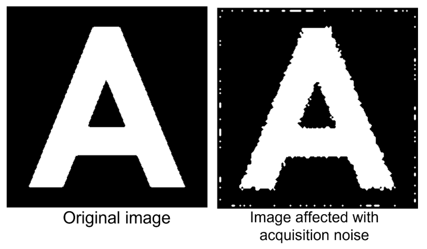
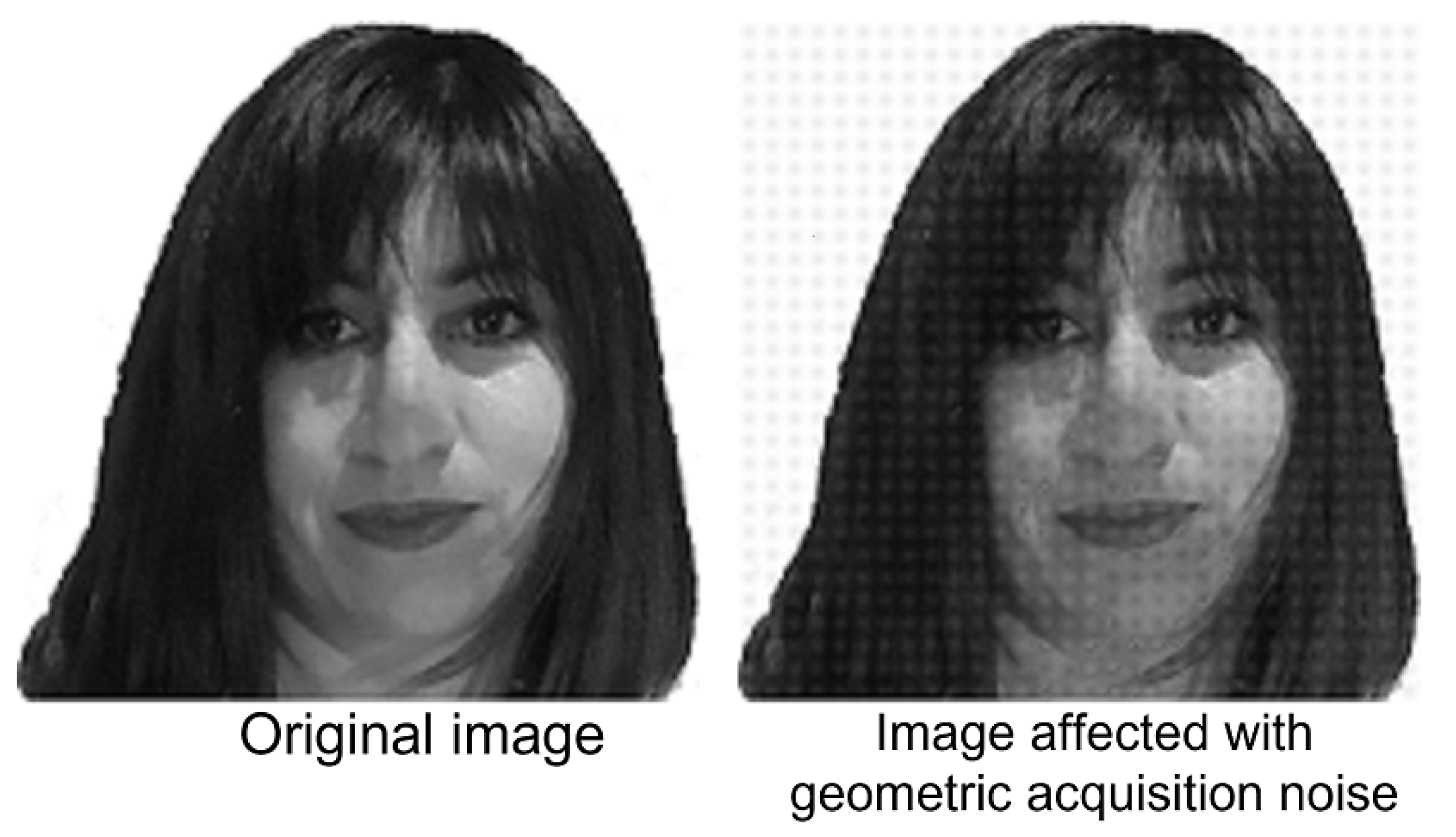
Section 3.2. We generated acquisition noise for binary images and geometric acquisition noise for gray-scale images, as detailed in Section 3.3.1 and 
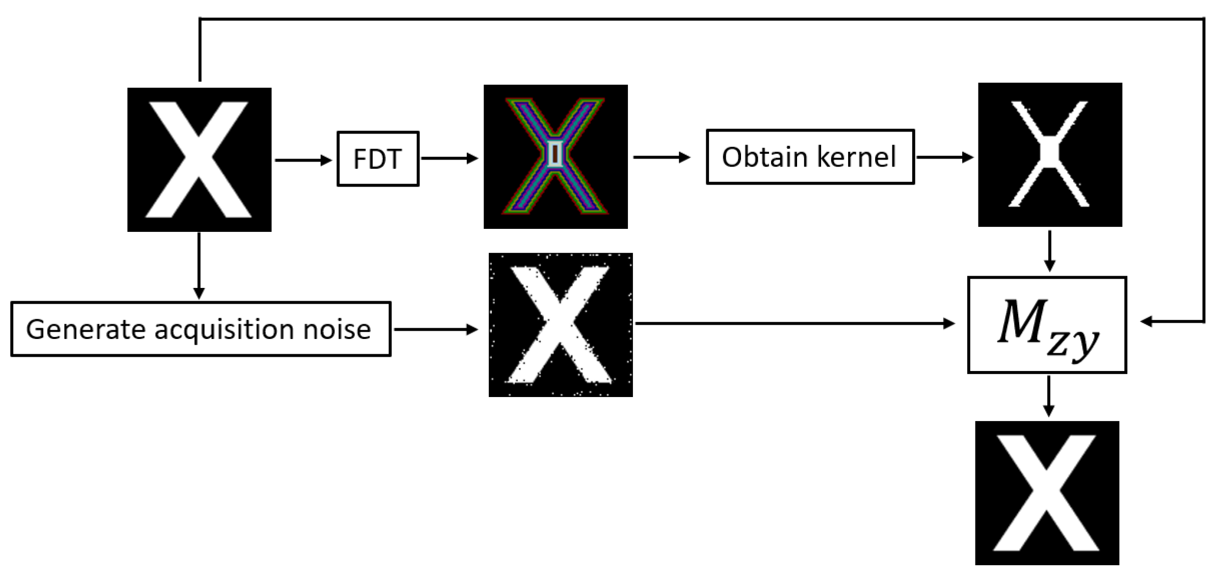
Section 3.3.2, respectively. To illustrate the process followed for binary patterns and gray-scale patterns in evaluating the performance of the generic maximum heteroassociative memory model, we have included Figure 23 and Figure 24.
According to the noise distribution proposed in [38], the percentages of noise distribution mapped to distances for binary images are specified in Table 1.
The Table 2 defines the percentages of noise distribution mapped to distances for binary images, where the total mixed noise up to distance d = 5 is 81 % . To create the kernel, a set of mapped pixels needs to be preserved at any distance d from the original pattern, where noise is less likely to alter them. Based on Theorem 3, it is possible to define the probability of the generic model of maximum heteroassociative memory completely recalling the patterns. The success probability is presented in Table 2.
The performance of the generic maximum heteroassociative memory model for fundamental set 1 is presented in Table 3. The recall percentage for a distance of 1 is above 70 % , which is very good for two reasons. Firstly, the expected probability of success for this distance is at least 19 % , which is met. Secondly, the original kernel model has 0 % recoveries with altered kernels with mixed noise. The expected probability of success can be defined by eliminating distance 1 and conserving distances 2 onward for kernel construction, which is 72 % . Table 3 shows that the generic max heteroassociative memory model meets the expected probability for distances 2, 3, and 4. From distance 5 onward, the pattern is recovered completely at 100 % . These results are in compliance with Theorem 3. 
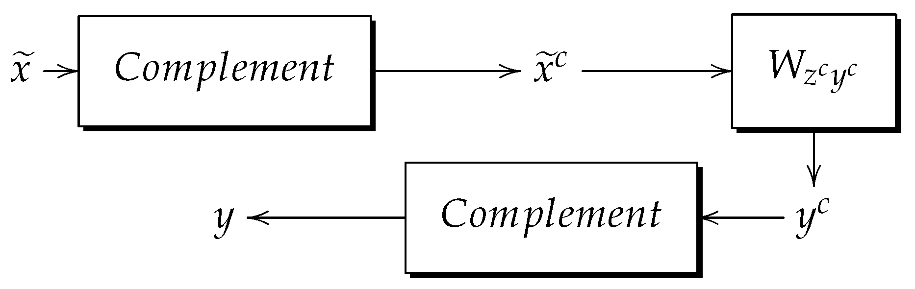
Table 3 also shows the percentages of complete recovery using the heteroassociative memory min, which meets the expected probability of success but has a lower recovery than the generic max heteroassociative memory model. This is because noise is presented where there is information, the more information there is, the more noise is presented. The kernel for the heteroassociative memory min works with the pattern complement, and because of the characteristics of the fundamental patterns used in this article, there is more information and therefore more noise, causing the heteroassociative memory to fail more times than the generic max heteroassociative memory model.
Table 4 demonstrates the performance of the generic heteroassociative memory max and confirms the results in Table 3 that meet the definition of Theorem 3, indicating the robustness of the generic model max to mixed noise. Although pattern H had the lowest performance in retrieval, it still satisfied Theorem 3. The minimum heteroassociative memories also performed well. These tables demonstrate that because the noise is concentrated at the edges, FDT enables the mapping of noise to the affected distances, making it easy to eliminate those distances affected by the noise. This approach facilitates the creation of kernels without noise, which would benefit the models of associative memories.
Table 5 is particularly interesting as it demonstrates the performance of max heteroassociative memories using binary images of faces. The recall percentages exceed what is expected according to Theorem 3. This type of image is particularly relevant for this type of memory as it tests its performance not with artificial patterns but with real patterns. As expected, min heteroassociative memories perform worse than generic heteroassociative memories max, as the creation of their kernel contains more information and therefore more noise.
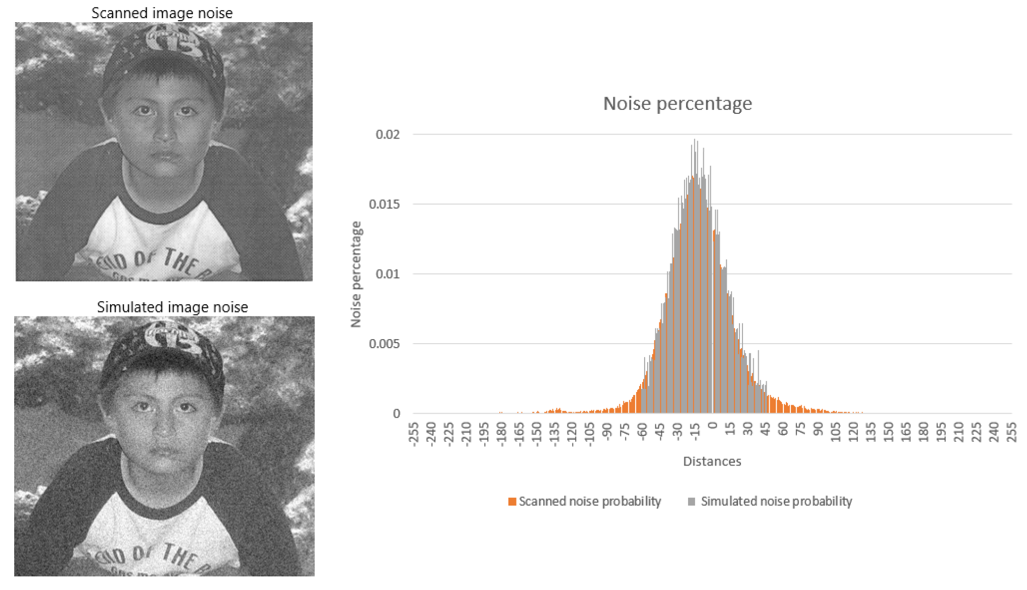
The probability distribution of mixed noise affecting distances in gray-scale images, as reported in ref. [38], ranges from distance 189 to distance 187, with their respective probabilities. This noise is concentrated at these distances, accounting for 100 % of the noise. Negative distances indicate additive noise, while positive distances indicate subtractive noise. To calculate the probability of complete recovery in the generic heteroassociative memory max, Theorem 3 must be applied. Table 6 displays the success rates for distances ranging from 10 to 100.
Table 7 demonstrates the performance of the generic max heteroassociative memory with fundamental set 4. Both memories exceed the expected probability of success in complete pattern recovery, as shown in Table 6. Furthermore, it is evident that the recall rate is 100 % from distance 35, indicating that both memories are robust to mixed noise. Overall, the proposed model meets expectations for all five fundamental sets.
Table 8 presents the performance of the max heteroassociative memory with the fundamental set 5. Despite the low performance observed for distances below 30, which did not meet the expected percentage shown in Table 6, the model is still valid. From a distance of 30 onward, it exceeds the expected success rate, demonstrating its robustness to mixed noise. The poor performance for distance 10 can be attributed to the 28 % probability of failure, but it does not invalidate the model. Although the minimum heteroassociative memory also performed well, it had lower performance than the generic max heteroassociative memory. As previously mentioned, the kernel created for the heteroassociative memory min uses the complement of the pattern, which leads to more information acquisition and subsequently more noise. This type of noise causes the associative memories in minmax algebra to fail.
The preceding results demonstrate a comparison between robust heteroassociative memory models, min and max, against mixed noise. It is evident that the generic max heteroassociative model outperforms the min heteroassociative model. The comparison was made using morphological associative memories, which offered the advantage of using both binary and grayscale images. The results indicate that the generic max heteroassociative memory model is not only faster, but it also builds the kernel with less information, resulting in a lower probability of noise interference and, therefore, a better performance than that of the robust heteroassociative model min against acquisition noise.
Having demonstrated that the generic model of max heteroassociative memory robust to acquisition noise outperforms the heteroassociative memory min model, we proceeded to apply the generic model of maximum heteroassociative memory to the maximum memory α β and to the max memory proposed by Gamino and Díaz-de-Leon (G-DL) [6]. We only did it for the binary case, as these memories are designed specifically for this purpose. The results of our experiment are presented in Table 9.
Table 9 indicates that the three memory models have very similar performance, which is not surprising given that they employ a generic model of maximum heteroassociative memory robust to acquisition noise and share the same fundamental set. The difference lies in the fact that Algorithm 1 generates acquisition noise randomly, resulting in distinct noise patterns for each iteration. Had the same noise patterns been applied to the generic model of maximum heteroassociative memory robust to acquisition noise across all three memory models, the results would likely have been virtually identical.
This demonstrates that the proposed model works effectively for any type of memory based on the minmax algebra, regardless of the type of operators utilized. Furthermore, the results indicate that the proposed model is superior to kernel generation models for existing minmax memories in the state of the art. Additionally, the method used to obtain the kernel aligns with the requirements of the original kernel model proposed by morphological memories. These findings suggest that, irrespective of the associative memory model employed, if the behavior of noise is known and can be mapped using a distance transform, it is feasible to create noise-free kernels. Furthermore, even when kernels are affected by noise, the proposed model offers a high probability of complete recall.
The patterns used in the fundamental set 4 are synthetic, but those in the fundamental set 5 are not. They are actual faces, which enhances the reliability of the generic heteroassociative memory max. The results demonstrate that the design of the max generic heteroassociative memory successfully meets its definitions, as its performance surpasses the expected percentages of success in pattern recovery. However, when the recalled patterns are not successful, they exhibit mixed noise, as demonstrated in Corollary 6. 
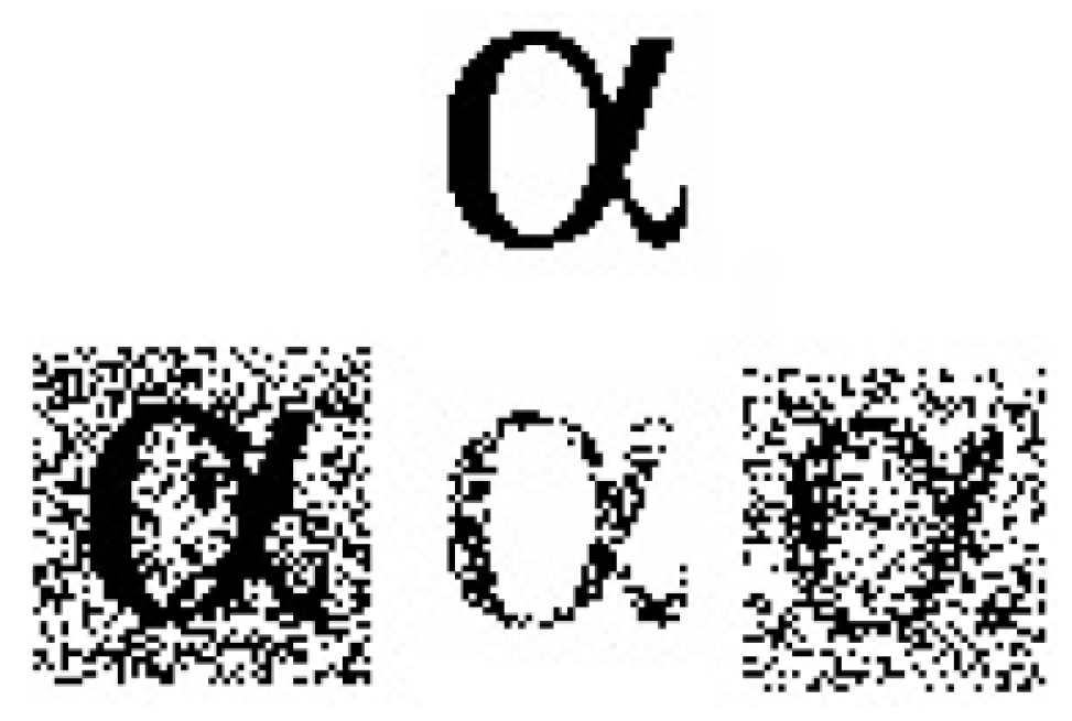
Figure 25 illustrates the appearance of poorly recovered patterns, confirming Corollary 6. Notably, the poorly recovered patterns retain many of the original pattern’s characteristics.

4. Discussion and Conclusions

Acquisition noise is known to appear, distribute, and grow at the edges of images. Nevertheless, it can be modeled using a Gaussian distribution through a distance transform. The distance transform has proved to be a useful tool for modeling acquisition noise in binary and gray-scale images.
It has been demonstrated that the generic maximum heteroassociative memory model achieves the expected probability of success in pattern recall. The generic model of max heteroassociative memory robust to acquisition noise allows patterns to be recalled even if the kernel is altered with mixed noise, whereas the original model does not allow for this. The minimum heteroassociative memory model shows superior results compared with the original model.
In order to verify its performance and advantages, the proposed model was compared with the then-new model of heteroassociative memory minimum robust to acquisition noise using morphological memory max. Table 3, Table 4 and Table 5 demonstrate that the proposed model performed better than the minimum heteroassociative model for the binary case. Moreover, the new model showed that for gray-scale images, it outperformed the heteroassociative min-memory model, as shown in Table 7 and Table 8. These results make it clear that the model of heteroassociative memory max robust to acquisition noise exceeds the heteroassociative memory min model.
To determine the performance of the proposed model of heteroassociative memory max robust to acquisition noise, three models of associative minmax memories were used: morphological, α β , and the memory proposed by Gamino and Díaz-de-León, all of which were designed to work in minmax algebra. The three memories were tested using the proposed model for the binary case, as the α β and G-DL memories were designed for this specific case. Table 9 shows that the morphological memories performed better than the other two memories, although the difference in recoveries is minimal. This may be attributed to the fact that the noise patterns to be retrieved are different for each attempt. These results demonstrate that the proposed model is functional for different associative memories in minmax algebra. In conclusion, the proposed model is functional for all associative memories in minmax algebra and outperforms the heteroassociative memory min model in robustness to acquisition noise.
Associative memories continue to be a topic of study for their applications in problem-solving in engineering. An example of this is the use of bidirectional discrete neural networks with associative memory (BAM) of the Cohen-Grossberg type for problems related to symmetry and their application in numerous engineering designs [47]. Additionally, associative memories have been applied in medicine, including non-invasive visual stimulation with EEG signals [48] and personalized frequency-modulated transcranial electrical stimulation for improving associative memory [49]. The practicality of using associative memories for problem-solving in various human endeavors is evident, which makes the current model of the maximum generic heteroassociative memory applicable to solving the aforementioned problems.

Author Contributions

Conceptualization, J.-C.S.-R.; validation, F.M.-G., J.-C.S.-R. and M.M.-I.; formal analysis, J.-C.S.-R., V.T.-M. and M.M.-I.; writing—original draft preparation, J.-C.S.-R. and V.T.-M.; writing—review and editing, F.M.-G., J.-C.S.-R., M.M.-I. and V.T.-M.; visualization, V.T.-M., F.M.-G. and J.-C.S.-R.; supervision, J.-C.S.-R. and M.M.-I. All authors have read and agreed to the published version of the manuscript.

Funding

This research received no external funding.

Data Availability Statement

Not applicable.

Acknowledgments

We thank the Universidad Politécnica de Pachuca, the Universidad Autonoma del Estado de México, the Centro de Investigación en Computación and CONACYT for the support provided.

Conflicts of Interest

The authors declare no conflict of interest.

References

  1. Bosch, H.; Kurfess, F. Information storage capacity of incompletely connected associative memories. Neural Netw. 1998, 11, 869–876. [Google Scholar] [CrossRef] [PubMed]
  2. Ritter, G.X.; Sussner, P.; Diaz-de-Leon, J. Morphological associative memories. IEEE Trans. Neural Netw. 1998, 9, 281–293. [Google Scholar] [CrossRef] [PubMed]
  3. Ritter, G.X.; Diaz-de-Leon, J.; Sussner, P. Morphological bidirectional associative memories. IEEE Neural Netw. 1999, 12, 851–867. [Google Scholar] [CrossRef] [PubMed]
  4. Santana, A.X.; Valle, M. Max-plus and min-plus projection autoassociative morphological memories and their compositions for pattern classification. Neural Netw. 2018, 100, 84–94. [Google Scholar]
  5. Sussner, P. Associative morphological memories based on variations of the kernel and dual kernel methods. Neural Netw. 2003, 16, 625–632. [Google Scholar] [CrossRef] [PubMed]
  6. Gamino, A.; Díaz-de-León, J. A new method to build an associative memory model. IEEE Lat. Am. Trans. 2021, 19, 1692–1701. [Google Scholar] [CrossRef]
  7. Yiannis, B. A new method for constructing kernel vectors in morphological associative memories of binary patterns. Comput. Sci. Inf. Syst. 2011, 8, 141–166. [Google Scholar] [CrossRef]
  8. Yong, K.; Pyo, G.; Sik, D.; Ho, D.; Jun, B.; Ryoung, K.; Kim, J. New iris recognition method for noisy iris images. Pattern Recognit. Lett. 2012, 33, 991–999. [Google Scholar]
  9. Aldape-Pérez, M.; Yáñez-Márquez, C.; López-Yáñez, I.; Camacho-Nieto, O.; Argüelles-Cruz, A. Collaborative learning based on associative models: Application to pattern classification in medical datasets. Comput. Hum. Behav. 2015, 51, 771–779. [Google Scholar] [CrossRef]
  10. Aldape-Pérez, M.; Alarcón-Paredes, A.; Yáñez-Márquez, C.; López-Yáñez, I.; Camacho-Nieto, O. An Associative Memory Approach to Healthcare Monitoring and Decision Making. Sensors 2018, 18, 2960. [Google Scholar] [CrossRef]
  11. Masuyama, N.; Islam, N.; Seera, M.; Kiong, C. Application of emotion affected associative memory based on mood congruency effects for a humanoid. Neural Comput. Appl. 2017, 28, 737–752. [Google Scholar] [CrossRef]
  12. Tarkov, M.S. Oscillatory neural associative memories with synapses based on memristor bridges. Opt. Mem. Neural Netw. 2016, 25, 219–227. [Google Scholar] [CrossRef]
  13. Knoblauch, A. Neural associative memory with optimal bayesian learning. Neural Comput. 2011, 23, 1393–1451. [Google Scholar] [CrossRef] [PubMed]
  14. Rendeiro, D.; Sacramento, J.; Wichert, A. Taxonomical associative memory. Cogn. Comput. 2014, 6, 45–65. [Google Scholar] [CrossRef]
  15. Heusel, J.; Löwe, M.; Vermet, F. On the capacity of an associative memory model based on neural cliques. Stat. Probab. Lett. 2015, 106, 256–261. [Google Scholar] [CrossRef]
  16. Acevedo-Mosqueda, M.; Yáñez-Márquez, C.; López-Yáñez, I. Alpha-Beta bidirectional associative memories: Theory and applications. Neural Process. Lett. 2007, 26, 1–40. [Google Scholar] [CrossRef]
  17. Acevedo, M.E.; Yáñez-Márquez, C.; Acevedo, M.A. Bidirectional associative memories: Different approaches. Acm Comput. Surv. 2013, 45, 1–30. [Google Scholar] [CrossRef]
  18. Yáñez-Márquez, C.; López-Yáñez, I.; Aldape-Pérez, M.; Camacho-Nieto, O.; Argüelles-Cruz, A.; Villuendas-Rey, Y. Theoretical Foundations for the Alpha-Beta Associative Memories: 10 Years of Derived Extensions, Models, and Applications. Neural Process. Lett. 2018, 48, 811–847. [Google Scholar] [CrossRef]
  19. Luna-Benoso, B.; Flores-Carapia, R.; Yáñez-Márquez, C. Associative memories based on cellular automata: An application to pattern recognition. Appl. Math. Sci. 2013, 7, 857–866. [Google Scholar] [CrossRef]
  20. Tchapet, J.; Njafa, S.G.; Engo, N. Quantum associative memory with linear and non-linear algorithms for the diagnosis of some tropical diseases. Neural Netw. 2018, 97, 1–10. [Google Scholar] [CrossRef]
  21. Zhu, Z.; You, X.; Philip, Z. An adaptive hybrid pattern for noise-robust texture analysis. Pattern Recognit. 2015, 48, 2592–2608. [Google Scholar] [CrossRef]
  22. Kim, H.; Hwang, S.; Park, J.; Yun, S.; Lee, J.; Park, B. Spiking Neural Network Using Synaptic Transistors and Neuron Circuits for Pattern Recognition With Noisy Images. IEEE Electron. Device Lett. 2018, 39, 630–633. [Google Scholar] [CrossRef]
  23. Peng, X.; Wen, J.; Li, Z.; Yang, G. Rough Set Theory Applied to Pattern Recognition of Partial Discharge in Noise Affected Cable Data. IEEE Trans. Dielectr. Electr. Insul. 2017, 24, 147–156. [Google Scholar] [CrossRef]
  24. Steinbuch, K. Die Lernmatrix. Kybernetik 1961, 1, 36–45. [Google Scholar] [CrossRef]
  25. Willshaw, D.; Buneman, O.; Longuet-Higgins, H. Non-holographic associative memory. Nature 1969, 222, 960–962. [Google Scholar] [CrossRef]
  26. Amari, S. Learning patterns and pattern sequences by self-organizing nets of threshold elements. IEEE Trans. Comput. 1972, C-21, 1197–1206. [Google Scholar] [CrossRef]
  27. Anderson, J.A. A simple neural network generating an interactive memory. Math. Biosci. 1972, 14, 197–220. [Google Scholar] [CrossRef]
  28. Kohonen, T. Correlation matrix memories. IEEE Trans. Comput. 1972, 100, 353–359. [Google Scholar] [CrossRef]
  29. Nakano, K. Associatron-A model of associative memory. IEEE Trans. Syst. Man. Cybern. 1972, SMC-2, 380–388. [Google Scholar] [CrossRef]
  30. Kohonen, T.; Ruohonen, M. Representation of associated data by matrix operators. IEEE Trans. Comput. 1973, c-22, 701–702. [Google Scholar] [CrossRef]
  31. Kohonen, T.; Ruohonen, M. An adaptive associative memory principle. IEEE Trans. Comput. 1973, c-24, 444–445. [Google Scholar] [CrossRef]
  32. Anderson, J.A.; Silverstein, J.; Ritz, S.; Jones, R. Distinctive features, categorical perception, and probability learning: Some applications of a neural model. Psichol. Rev. 1977, 84, 413–451. [Google Scholar] [CrossRef]
  33. Amari, S. Neural theory of association and concept-formation. Biol. Cybern. 1977, 26, 175–185. [Google Scholar] [CrossRef] [PubMed]
  34. Hopfield, J. Neural networks and physical systems with emergent collective computational abilities. Proc. Natl. Acad. Sci. USA 1982, 79, 2554–2558. [Google Scholar] [CrossRef]
  35. Hopfield, J. Neurons with graded respose have collective computational properties like those of two-state neurons. Proc. Natl. Acad. Sci. USA 1984, 81, 3088–3092. [Google Scholar] [CrossRef]
  36. Karpov, Y.L.; Karpov, L.E.; Smetanin, Y.G. Associative Memory Construction Based on a Hopfield Network. Program. Comput. Softw. 2020, 46, 305–311. [Google Scholar] [CrossRef]
  37. Sussner, P. Observations on morphological associative memories and the kernel method. Neurocomputing 2000, 31, 167–183. [Google Scholar] [CrossRef]
  38. Salgado-Ramírez, J.C.; Vianney Kinani, J.M.; Cendejas-Castro, E.A.; Rosales-Silva, A.J.; Ramos-Díaz, E.; Díaz-de-Léon-Santiago, J.L. New Model of Heteroasociative Min Memory Robust to Acquisition Noise. Mathematics 2022, 10, 148. [Google Scholar] [CrossRef]
  39. Estevão, E.; Sussner, P.; Bustince, H.; Fernández, J. Theta-Fuzzy Associative Memories (Theta-FAMs). IEEE Trans. Fuzzy Syst. 2015, 23, 313–326. [Google Scholar] [CrossRef]
  40. Estevão, E.; Sussner, P.; Sandri, S. Tunable equivalence fuzzy associative memories. Fuzzy Sets Syst. 2016, 292, 242–260. [Google Scholar]
  41. Díaz de León, J.L.; Gamino Carranza, A. New binary associative memory model based on the XOR operation. AAECC 2022, 33, 283–320. [Google Scholar] [CrossRef]
  42. Xiao, Y.; Zeng, J.; Michael, Y. Restoration of images corrupted by mixed Gaussian-impulse noise via l1–l0 minimization. Pattern Recognit. 2011, 44, 1708–1720. [Google Scholar] [CrossRef]
  43. Chervyakov, N.; Lyakhov, P.; Kaplun, D.; Butusov, D.; Nagornov, N. Analysis of the Quantization Noise in Discrete Wavelet Transform Filters for Image Processing. Electronics 2018, 7, 135. [Google Scholar] [CrossRef]
  44. Fan, Y.; Zhang, L.; Guo, H.; Hao, H.; Qian, K. Image Processing for Laser Imaging Using Adaptive Homomorphic Filtering and Total Variation. Photonics 2020, 7, 30. [Google Scholar] [CrossRef]
  45. Liu, D.; Wen, B.; Jiao, J.; Liu, X.; Wang, Z.; Huang, T.S. Connecting Image Denoising and High-Level Vision Tasks via Deep Learning. IEEE Trans. Image Process. 2020, 29, 3695–3706. [Google Scholar] [CrossRef]
  46. Khan, A.; Jin, W.; Haider, A.; Rahman, M.; Wang, D. Adversarial Gaussian Denoiser for Multiple-Level Image Denoising. Sensors 2021, 21, 2998. [Google Scholar] [CrossRef]
  47. Stamov, T. Discrete Bidirectional Associative Memory Neural Networks of the Cohen–Grossberg Type for Engineering Design Symmetry Related Problems: Practical Stability of Sets Analysis. Symmetry 2022, 14, 216. [Google Scholar] [CrossRef]
  48. Bjekić, J.; Paunovic, D.; Živanović, M.; Stanković, M.; Griskova-Bulanova, I.; Filipović, S.R. Determining the Individual Theta Frequency for Associative Memory Targeted Personalized Transcranial Brain Stimulation. J. Pers. Med. 2022, 12, 1367. [Google Scholar] [CrossRef]
  49. Bjekić, J.; Živanović, M.; Paunović, D.; Vulić, K.; Konstantinović, U.; Filipović, S.R. Personalized Frequency Modulated Transcranial Electrical Stimulation for Associative Memory Enhancement. Brain Sci. 2022, 12, 472. [Google Scholar] [CrossRef]
Figure 1. Associative memories phases.
Mathematics 11 02015 g001
Figure 2. Additive noise, subtractive noise, and mixed noise, respectively.
Mathematics 11 02015 g002
Figure 5. Learning process of the minimum heteroassociative memory model.
Mathematics 11 02015 g005
Figure 6. Recall process of the model of min heteroassociative memories.
Mathematics 11 02015 g006
Figure 9. Left image is binary image and right image is the FDT.
Mathematics 11 02015 g009
Figure 10. Left image is a binary image and right image is the FDT.
Mathematics 11 02015 g010
Figure 11. The image on the left is the original gray-scale image, while the image on the right is the noise image.
Mathematics 11 02015 g011
Figure 12. Noise scheme.
Mathematics 11 02015 g012
Figure 13. Schema for obtaining the noiseless Kernel.
Mathematics 11 02015 g013
Figure 14. Learning process of the model of maximum heteroassociative memories.
Mathematics 11 02015 g014
Figure 15. Recalling process of the model of max heteroassociative memories.
Mathematics 11 02015 g015
Figure 19. The distribution of absolute and relative frequencies of acquisition noise in binary images.
Mathematics 11 02015 g019
Figure 20. Process of generating patterns with acquisition noise.
Mathematics 11 02015 g020
Figure 21. Scanned image vs simulated image noise distributions.
Mathematics 11 02015 g021
Figure 22. Binary image as result of difference between original image and noise image.
Mathematics 11 02015 g022
Figure 23. Visual scheme of generic max heteroassociative memory for binary images.
Mathematics 11 02015 g023
Figure 24. Visual scheme of generic max heteroassociative memory for gray-scale images.
Mathematics 11 02015 g024
Figure 25. Failed patterns recalled.
Mathematics 11 02015 g025
Table 1. Acquisition noise distribution in binary images.
fromtoNoise Probabilities SumAcumulated Noise
distances 1 1 0.5 0.5
distances 2 2 0.15 0.65
distances 3 3 0.08 0.73
distances 4 4 0.05 0.78
distances 5 5 0.03 0.81
Table 2. Probability of complete recalling success in binary images.
fromtoRecalling Success Probability
distances15 1 0.81 = 0.19
distances25 1 0.27 = 0.73
distances35 1 0.16 = 0.84
distances45 1 0 . 0.8 = 0.92
distances55 1 0.03 = 0.97
Table 3. Performance of the generic max model vs. min model in fundamental set 1.
Max ModelMin Model
Pattern d = 1 d = 2 d = 3 d = 4 d = 5 d = 1 d = 2 d = 3 d = 4 d = 5
a74.1%80.7%92.9%99.3%100%70.8%78.2%90.1%97.1%100%
f72.6%82.9%91.0%98.9%100%70.3%80.9%89.8%95.8%100%
j76.8%83.0%95.4%99.7%100%74.2%81.1%90.8%98.3%100%
p73.1%81.6%91.3%99.3%100%71.8%78.9%90.3%97.7%100%
y77.9%83.6%98.2%100%100%75.3%79.8%98.1%98.4%100%
Table 4. Performance of the generic max model vs. min model in fundamental set 2.
Max ModelMin Model
Pattern d = 1 d = 2 d = 3 d = 4 d = 5 d = 1 d = 2 d = 3 d = 4 d = 5
A80.5%85.1%90.8%98.4%100%78.9%83.6%89.9%96.3%100%
H57.3%88.7%94.4%93.9%100%56.8%83.9%90.7%97.8%100%
T84.9%94.8%90.7%99.3%100%80.8%90.7%87.9%97.3%100%
X69.7%81.3%92.7%93.5%100%66.9%79.7%90.8%91.6%100%
Table 5. Performance of the generic max model vs. min model in fundamental set 3.
Max ModelMin Model
Pattern d = 1 d = 2 d = 3 d = 4 d = 5 d = 1 d = 2 d = 3 d = 4 d = 5
binary142.7%75.9%88.4%86.2%100%39.6%87.2%88.1%85.9%100%
binary277.6%89.0%93.6%99.8%100%70.5%88.2%92.7%99.2%100%
binary363.2%84.1%87.8%96.5%100%62.9.1%83.2%96.2%96.5%100%
Table 6. Probability of complete recovery success.
fromtoNoise Probabilities SumSuccess Probability
distances101870.281 − 0.28 = 0.72
distances201870.221 − 0.22 = 0.78
distances301870.161 − 0.16 = 0.84
distances401870.121 − 0.12 = 0.88
distances501870.091 − 0.09 = 0.91
distances601870.071 − 0.07 = 0.93
distances701870.051 − 0.05 = 0.95
distances801870.031 − 0.03 = 0.97
distances901870.021 − 0.02 = 0.98
distances1001870.021 − 0.02 = 0.98
Table 7. Performance of the generic max model vs. min model in fundamental set 4.
Max ModelMin Model
Pattern d = 10 d = 30 d = 35 d = 10 d = 30 d = 35
A75.1%92.3%100%74.9%90.8%100%
B72.7%90.8%100%71.4%90.0%100%
E77.8%97.9%100%76.1%96.2%100%
Q78.3%98.2%100%77.2%96.9%100%
Table 8. Performance of the generic max model vs. min model in fundamental set 5.
Max ModelMin Model
Pattern d = 10 d = 30 d = 35 d = 10 d = 30 d = 35
gray119.6%95.6%100%18.9%93.7%100%
gray224.9%93.5%100%24.4%91.6%100%
gray387.2%99.1%100%77.9%97.3%100%
Table 9. Performance of the generic model on morphological memories, α β , and G-DL using fundamental set 2.
Morphological α β G-DL
Pattern d = 1 d = 2 d = 3 d = 4 d = 5 d = 1 d = 2 d = 3 d = 4 d = 5 d = 1 d = 2 d = 3 d = 4 d = 5
A80.5%85.1%90.8%98.4%100%80.1%85.3%90.2%97.6%100%80.7%89.9%97.9%98.2%100%
H57.3%88.7%94.4%93.9%100%57.4%87.6%94.7%93.1%100%56.9%93.8%93.4%93.7%100%
T84.9%94.8%90.7%99.3%100%84.1%94.3%90.3%98.9%100%83.7%94.8%99.5%99.5%100%
X69.7%81.3%92.7%93.5%100%68.3%81.0%93.2%93.4%100%69.2%81.5%92.8%93.7%100%
Disclaimer/Publisher’s Note: The statements, opinions and data contained in all publications are solely those of the individual author(s) and contributor(s) and not of MDPI and/or the editor(s). MDPI and/or the editor(s) disclaim responsibility for any injury to people or property resulting from any ideas, methods, instructions or products referred to in the content.

