Optical Solitons for the Concatenation Model with Differential Group Delay: Undetermined Coefficients

Abstract

In the current study, the concatenation model of birefringent fibers is explored for the first time, and we present optical soliton solutions to the model. The integration algorithm used to achieve this retrieval is the method of undetermined coefficients, which yields a wide range of soliton solutions. The parameter constraints arise naturally during the derivation of the soliton solutions, which are essential for such solitons to exist.

1. Introduction

While there exists an abundance of models that govern the propagation of solitons across transcontinental and transoceanic distances through an optical fiber, an interesting equation that was proposed about a decade ago in 2014 by Ankiewicz et al. is the concatenation model [1,2]. This model is a combination of three well-known equations that describe the dynamics of soliton transmission across intercontinental distances. They are the nonlinear Schrödinger Equation (NLSE), the Lakshmanan–Porsezian–Daniel (LPD) model, and the Sasa–Satsuma Equation (SSE). These three models are concatenated in sequence, hence the name.

Recently, the concatenation model has gained further importance and has attracted considerable attention from a wide range of perspectives. The soliton solutions were derived through the use of undetermined coefficients. The conservation laws were also enumerated after they were identified by the multiplier approach. The model was also addressed numerically with the Laplace–Adomian decomposition scheme. The trial equation approach was also implemented, and Painleve analysis was carried out [3,4,5,6,7]. These studies were all conducted for the scalar version of the model. It is now time to turn the page and move on.

The current paper addresses the concatenation model in birefringent fibers, again with the help of undetermined coefficients. A full spectrum of solitons is thus made available, along with the solvability conditions, which are listed as parameter constraints. After providing a brief introduction to the model in birefringent fibers, in the rest of the paper, we explain the derivation of these solitons in detail using the integration algorithm. The results are then presented with full transparency.

Governing Model

The concatenation model for polarization-preserving fibers can be stated as follows:

$$\begin{array}{ccc}\hfill i{u}_t+a{u}_{xx}+b{\left|u\right|}^{2}u& +& c_1\left[{\sigma }_1{u}_{xxxx}+{\sigma }_2{\left(u_x\right)}^2{u}^{*}+{\sigma }_3{\left|u_x\right|}^{2}u+{\sigma }_4{\left|u\right|}^2{u}_{xx}+{\sigma }_5{u}^2{u}_{xx}^{*}+{\sigma }_6{\left|u\right|}^{4}u\right]\hfill \\ & +& i{c}_2\left[{\sigma }_7{u}_{xxx}+{\sigma }_8{\left|u\right|}^2{u}_x+{\sigma }_9{u}^2{u}_x^{*}\right]=0.\hfill \end{array}$$

(1)

Equation (1) is the concatenation model that is formed by joining three well-studied models in fiber optics, namely NLSE, the LPD equation, and the SSE. It must be noted that when $c_1=c_2=0$, we have the NLSE; while if $c_1=0$, we recover the SSE; and when $c_2=0$, we obtain the LPD model. Thus, Equation (1), as it stands, is the model that is generated by concatenating the three globally familiar models from nonlinear fiber optics.

For birefringent fibers, Equation (1) is split into two components as:

$$\begin{array}{ccc}& & i{q}_t+a_1{q}_{xx}+\left(b_1{\left|q\right|}^2+c_1{\left|r\right|}^2\right)q\hfill \\ & +& c_{11}\left[{\sigma }_{11}{q}_{xxxx}+\left\{{\alpha }_1{\left(q_x\right)}^2+{\beta }_1{\left(r_x\right)}^2\right\}{q}^{*}+\left({\gamma }_1{\left|q_x\right|}^2+{\lambda }_1{\left|r_x\right|}^2\right)q+\left({\delta }_1{\left|q\right|}^2+{\zeta }_1{\left|r\right|}^2\right)q_{xx}\right.\hfill \\ & +& \left.\left({\mu }_1{q}^2+{\rho }_1{r}^2\right)q_{xx}^{*}+\left(f_1{\left|q\right|}^4+g_1{\left|q\right|}^2{\left|r\right|}^2+h_1{\left|r\right|}^4\right)q\right]\hfill \\ & +& i{c}_{21}\left[{\sigma }_{71}{q}_{xxx}+\left({\eta }_1{\left|q\right|}^2+{\theta }_1{\left|r\right|}^2\right)q_x+\left({\epsilon }_1{q}^2+{\tau }_1{r}^2\right)q_x^{*}\right]=0,\hfill \end{array}$$

(2)

and

$$\begin{array}{ccc}& & i{r}_t+a_2{r}_{xx}+\left(b_2{\left|r\right|}^2+c_2{\left|q\right|}^2\right)r\hfill \\ & +& c_{12}\left[{\sigma }_{12}{r}_{xxxx}+\left\{{\alpha }_2{\left(r_x\right)}^2+{\beta }_2{\left(q_x\right)}^2\right\}{r}^{*}+\left({\gamma }_2{\left|r_x\right|}^2+{\lambda }_2{\left|q_x\right|}^2\right)r+\left({\delta }_2{\left|r\right|}^2+{\zeta }_2{\left|q\right|}^2\right)r_{xx}\right.\hfill \\ & +& \left.\left({\mu }_2{r}^2+{\rho }_2{q}^2\right)r_{xx}^{*}+\left(f_2{\left|r\right|}^4+g_2{\left|r\right|}^2{\left|q\right|}^2+h_2{\left|q\right|}^4\right)r\right]\hfill \\ & +& i{c}_{22}\left[{\sigma }_{72}{r}_{xxx}+\left({\eta }_2{\left|r\right|}^2+{\theta }_2{\left|q\right|}^2\right)r_x+\left({\epsilon }_2{r}^2+{\tau }_2{q}^2\right)r_x^{*}\right]=0.\hfill \end{array}$$

(3)

Equations (2) and (3) represent the concatenation model split into two components for a birefringent fiber. For $j=1,2$, $a_j$ represents the chromatic dispersion along the two components, while $b_j$ accounts for self-phase modulation, and $c_j$ represents the cross-phase modulation. Then, ${\sigma }_{1j}$ represents the fourth-order dispersions along the two components. Next up, ${\alpha }_j$, ${\beta }_j$, ${\gamma }_j$, ${\lambda }_j$, ${\delta }_j$, ${\zeta }_j$, ${\mu }_j$, ${\rho }_j$, $f_j$, $g_j$, and $h_j$ are the respective split-ups of the coefficients ${\sigma }_2$ to ${\sigma }_6$ from the LPD model, along the two components for a birefringent fiber. ${\sigma }_{7j}$ represents the coefficients of the fourth-order dispersion along the components, while in Equation (1), this effect is represented by the coefficient of ${\sigma }_7$. Finally, ${\eta }_j$, ${\theta }_j$, ${ϵ}_j$, and ${\tau }_j$ are the components of soliton self-frequency shift along the two components of a birefringent fiber, which are designated by ${\sigma }_8$ and ${\sigma }_9$ in the SSE part.

The concatenation model of (2) and (3) describes the propagation of solitons in birefringent optical fibers. It is composed of three main equations, namely the NLSE, the LPD model, and the SSE. These three equations are concatenated or combined to form a more comprehensive model that can describe the behavior of solitons in a wide range of situations. The NLSE is a fundamental equation in nonlinear optics and describes the propagation of light in a medium with a nonlinear refractive index. It is used to model the propagation of solitons in fiber optic communication systems. The LPD model is a modified version of the NLSE that includes additional terms to account for the effects of birefringence, which is the property of a medium that causes light to split into two polarized components. This model is used to study the behavior of solitons in birefringent fibers. The SSE is another important equation in soliton theory that describes the propagation of solitons in dispersive media. It is a generalization of the NLSE and is used to study the behavior of solitons in media with higher-order dispersion.

By combining these three equations into a single model, the concatenation model provides a more complete and accurate description of the behavior of solitons in birefringent optical fibers. It has many applications in fiber optic communication systems, where solitons are used to transmit information over long distances with minimal distortion.

It must be noted that the preliminary model was introduced about a decade ago [1,2]. It is not yet known what the exact form of an optical fiber would be or where such a form would be applicable. With a conjecture that it would make sense for erbium-doped fiber, in the present study, the governing model (1) is split and considered with differential group delay for the first time. This is proposed as a purely analytical model before any laboratory testing.

The integration of the coupled system (2) and (3) requires the following hypothesis to be applied:

$$\begin{array}{c}\hfill q(x,t)=P_1(x,t)e^{i\left(-\kappa x+\omega t+\Theta \right)},\end{array}$$

(4)

and

$$\begin{array}{c}\hfill r(x,t)=P_2(x,t)e^{i\left(-\kappa x+\omega t+\Theta \right)}.\end{array}$$

(5)

On the basis of this hypothesis, the waveform is described by the function $P(x,t)$, which is unique for each type of soliton; $\Theta$ is a phase constant; the wave number is represented by $\omega$; and the soliton frequency is given by $\kappa$. Inserting these hypotheses into (2) and (3) leads to the real part identity

$$\begin{array}{ccc}& & -[\omega +{\kappa }^2{a}_l+{\kappa }^3(c_{2l}{\sigma }_{7l}-\kappa c_{1l}{\sigma }_{1l})]P_l+[b_l-\kappa c_{2l}({\epsilon }_l-{\eta }_l)-{\kappa }^2{c}_{1l}({\alpha }_l-{\gamma }_l+{\delta }_l+{\mu }_l)]P_l^3\hfill \\ & & +c_{1l}{f}_l{P}_l^5+c_{1l}{g}_l{P}_l^3{P}_2^2+c_{1l}{h}_l{P}_l{P}_{\overline{l}}^4+[c_l-\kappa (\kappa c_{1l}({\beta }_l+{\xi }_l+{\rho }_l-{\lambda }_l)+c_{2l}({\tau }_l-{\theta }_l))]P_l{P}_{\overline{l}}^2\hfill \\ & & +c_{1l}({\alpha }_l+{\gamma }_l)P_l{\left(\frac{\partial P_l}{\partial x}\right)}^2+c_{1l}({\beta }_l+{\lambda }_l)P_l{\left(\frac{\partial P_{\overline{l}}}{\partial x}\right)}^2+c_{1l}[({\delta }_l+{\mu }_l)P_l^2+({\xi }_l+{\rho }_l)P_{\overline{l}}^2]\frac{{\partial }^2{P}_l}{\partial x^2}\hfill \\ & & +[a_l+3\kappa (c_{2l}{\sigma }_{7l}-2\kappa c_{1l}{\sigma }_{1l})]\frac{{\partial }^2{P}_l}{\partial x^2}+c_{1l}{\sigma }_{1l}\frac{{\partial }^4{P}_l}{\partial x^4}=0,\hfill \end{array}$$

(6)

while the imaginary counterpart reduces to

$$\begin{array}{ccc}& & \frac{\partial P_l}{\partial t}-[2\kappa a_l-(4k{c}_{1l}{\sigma }_{1l}-3c_{2l}{\sigma }_{7l}){\kappa }^2]\frac{\partial P_l}{\partial x}+[c_{2l}({\epsilon }_l+{\eta }_l)-2\kappa c_{1l}({\alpha }_l+{\delta }_l-{\mu }_l)]P_l^2\frac{\partial P_l}{\partial x}\hfill \\ & & +[c_{2l}({\theta }_l+{\tau }_l)-2\kappa c_{1l}({\xi }_l-{\rho }_l)]P_{\overline{l}}^2\frac{\partial P_l}{\partial x}-2\kappa {\beta }_l{c}_{1l}{P}_l{P}_{\overline{l}}\frac{\partial P_{\overline{l}}}{\partial x}+(c_{2l}{\sigma }_{7l}-4\kappa c_{1l}{\sigma }_{1l})\frac{\partial P_l}{\partial x^3}=0,\hfill \end{array}$$

(7)

where $\overline{l}=3-l$ and $l=1,2.$ Equation (7) shows that the speed can be retrieved as

$$v=-2\kappa (a_l+c_{2l}{\sigma }_{7l}\kappa ),$$

(8)

after considering

$$\begin{array}{ccc}& & c_{2l}({\epsilon }_l+{\eta }_l)=2\kappa c_{1l}({\alpha }_l+{\delta }_l-{\mu }_l),\hfill \end{array}$$

(9)

$$\begin{array}{ccc}& & c_{2l}({\theta }_l+{\tau }_l)=2\kappa c_{1l}(\xi -{\rho }_l),\hfill \end{array}$$

(10)

$$\begin{array}{ccc}& & {\beta }_l=0,\hfill \end{array}$$

(11)

$$\begin{array}{ccc}& & c_{2l}{\sigma }_{7l}=4\kappa c_{1l}{\sigma }_{1l}.\hfill \end{array}$$

(12)

Additionally, comparing the two values of the speed yields

$$a_1=a_2=a,c_{21}=c_{22}=c_7,{\sigma }_{71}={\sigma }_{72}={\sigma }_7.$$

(13)

Thus, as a direct consequence, the speed is rewritten as

$$v=-2\kappa (a+c_7{\sigma }_7\kappa ),$$

(14)

while in view of constraints (9)–(12), the real part of Equation (6) is recast as

$$\begin{array}{ccc}& & -(\omega +a{\kappa }^2+3c_{1l}{\sigma }_{1l}{\kappa }^4)P_l+[b_l-\kappa c_7({\epsilon }_l-{\eta }_l)-c_{1l}{\kappa }^2({\alpha }_l-{\gamma }_l+{\delta }_l+{\mu }_l)]P_l^3\hfill \\ & & +c_{1l}{f}_l{P}_l^5+c_{1l}{g}_l{P}_l^3{P}_{\overline{l}}^2+c_{1l}{h}_l{P}_l{P}_{\overline{l}}^4+[c_l-\kappa (\kappa c_{1l}({\xi }_l+{\rho }_l-{\lambda }_l)+c_7({\tau }_l-{\theta }_l))]P_l{P}_{\overline{l}}^2\hfill \\ & & +c_{1l}({\alpha }_l+{\gamma }_l)P_l{\left(\frac{\partial P_l}{\partial x}\right)}^2+c_{1l}{\lambda }_l{P}_l{\left(\frac{\partial P_{\overline{l}}}{\partial x}\right)}^2+c_{1l}[({\delta }_l+{\mu }_l)P_l^2+({\xi }_l+{\rho }_l)P_{\overline{l}}^2]\frac{{\partial }^2{P}_l}{\partial x^2}\hfill \\ & & +(a+6c_{1l}{\sigma }_{1l}{\kappa }^2)\frac{{\partial }^2{P}_l}{\partial x^2}+c_{1l}{\sigma }_{1l}\frac{{\partial }^4{P}_l}{\partial x^4}=0.\hfill \end{array}$$

(15)

It must be noted from (8) that the speeds of the solitons along the two components of a birefringent fiber appear to be different. This is because the parameters and coefficients are chosen generally. Then, equating the two components of the soliton velocity yields a number of parameter constraints and relations given by (13), leading to the recovery of the single speed at which the soliton travels along the two components, as expressed by (14).

Throughout the next section, we will explore the integrability of the real part Equation (15) from the point of view of four different types of soliton solutions.

2. Soliton Solutions

Soliton solutions are a type of mathematical solution that describes a self-reinforcing solitary wave that maintains its shape and velocity over a significant distance. These solutions arise in various fields, including physics, engineering, and applied mathematics, where they have important applications in areas such as optical fiber communications, plasma physics, and water waves. The study of solitons began in the 19th century when Scottish engineer John Scott Russell observed a solitary wave on a canal in Scotland. It was not until the 1960s, however, that the theory of solitons began to take shape with the development of the NLSE, which is a mathematical model that describes the behavior of solitons. Today, researchers continue to study soliton solutions in various settings, developing new models and methods for their analysis and application. The study of solitons remains an active area of research, with many new discoveries and applications expected in the years to come.

We now proceed to secure optical solitons with the concatenation model with differential group delay ((2) and (3)). Four different solitons are explored in the next four subsections by studying the integrability of the real part Equation (15) according to the corresponding waveform ($P_l(x,t)$).

The principle of undetermined coefficients is fairly simple. With an appropriate hypothesis of the soliton solutions that can be deciphered from the scalar version of the model, namely (1), the governing model is simplified after inserting this hypothesis into the two components. The real and imaginary components are separated. The imaginary component gives way to the velocity of the soliton, along with a few parameter constraints. The real part gives a relation from which the coefficients of the linearly independent functions are set to zero. This yields the relation between the soliton amplitude and width, along with a few more parameter constraints. Thus, a complete picture of the soliton, along with its essential parameter relations, is derived. It is applicable to bright, dark, and singular solitons. A transparent shortcoming of this approach is that it fails to recover soliton radiation and cannot be applied to derive multiple soliton solutions.

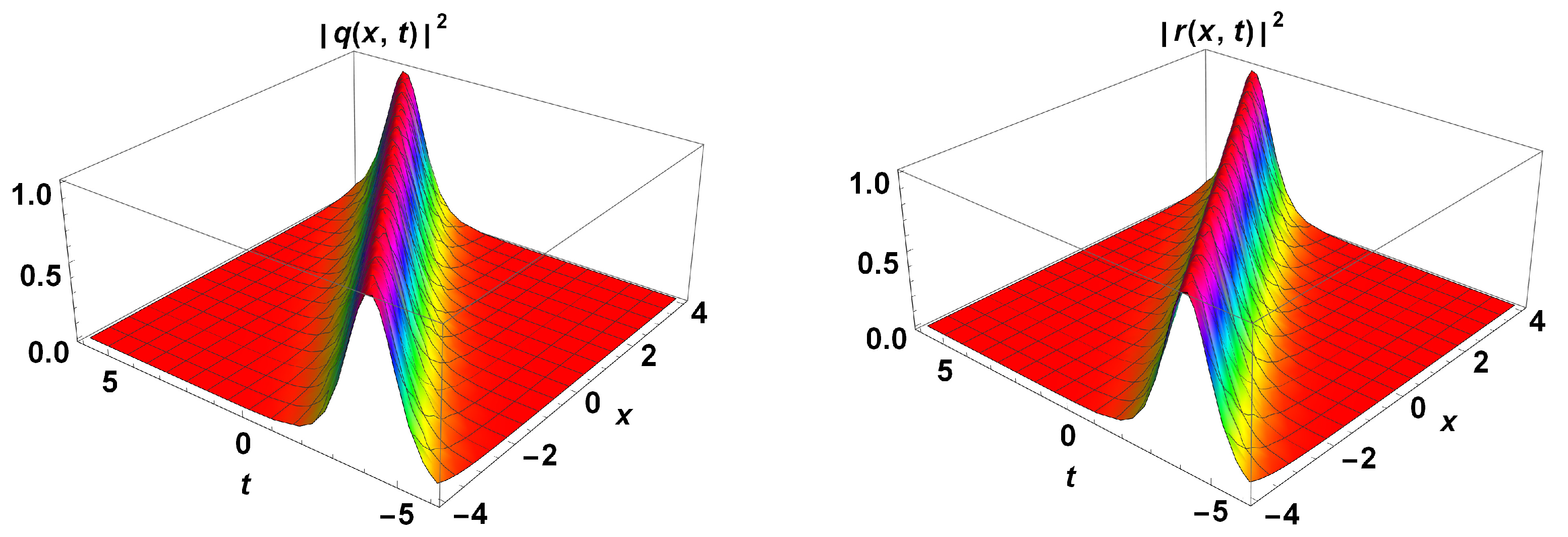
2.1. Bright Solitons

Bright solitons are a type of soliton solution that describes a self-reinforcing wave that has a maximum amplitude at its center. They are called “bright” solitons because they can be easily observed in optical systems, where they appear as bright pulses of light. Bright soliton solutions are important in many areas of physics, including fiber optics, plasma physics, and Bose–Einstein condensates. Bright soliton solutions are typically described by the NLSE, which is a mathematical model that takes into account the nonlinearity of the wave equation. These solutions are characterized by their ability to maintain their shape and velocity over long distances, and they are highly stable, making them ideal for use in telecommunications and other applications. The study of bright soliton solutions is an active area of research, with many new models and methods for their analysis and application. Researchers continue to explore the properties of these solutions in various settings, and new discoveries are expected to emerge in the years to come. Bright soliton solutions are a fascinating and important area of study in modern physics and applied mathematics.

The first case to be addressed is the bright soliton, this waveform of which typically has a structure of the form,

$$\begin{array}{c}\hfill P_l(x,t)=A_l{sech}^{p_l}\phi ,\phi =B(x-vt),\end{array}$$

(16)

where the soliton amplitudes $A_l$$(l=1,2)$ have a width of B, which implies that there are two soliton amplitudes with a specified width. The value of the unknown exponent ($p_l$) can be determined using the principle of balance. By plugging the expression (16) into Equation (15), we obtain a simplified form of the equation,

$$\begin{array}{ccc}& & [p_l^2(a_l+6c_{1l}{\sigma }_{1l}{\kappa }^2)B^2+p_l^4{c}_{1l}{\sigma }_{1l}{B}^2-(\omega +a{\kappa }^2+3c_{1l}{\sigma }_{1l}{\kappa }^4)]A_l{sech}^{p_l}\phi \hfill \\ & & +[(b_l-\kappa c_7({\epsilon }_l-{\eta }_l)-c_{1l}{\kappa }^2({\alpha }_l-{\gamma }_l+{\delta }_l+{\mu }_l))+p_l^2{c}_{1l}({\alpha }_l+{\gamma }_l+{\delta }_l+{\mu }_l)B^2]A_l^3{sech}^{3p_l}\phi \hfill \\ & & +f_l{c}_{1l}{A}_l^5{sech}^{5p_l}\phi -p_p(1+p_l)[(a+6c_{1l}{\sigma }_{1l}{\kappa }^2)+2c_{1l}{\sigma }_{1l}(2+p_l(2+p_l))B^2]A_l{B}^2{sech}^{2+p_l}\phi \hfill \\ & & +p_l(1+p_l)(2+p_l)(3+p_l)c_{1l}{\sigma }_{1l}{A}_l{B}^4{sech}^{4+p_l}\phi -p_l[p_l{c}_{1l}({\alpha }_l+{\gamma }_l)+(1+p_l)c_{1l}({\delta }_l+{\mu }_l)]A_l^3{B}^2{sech}^{2+3p_l}\phi \hfill \\ & & +\{[c_l-\kappa (\kappa c_{1l}({\xi }_l+{\rho }_l-{\lambda }_l)+c_7({\tau }_l-{\theta }_l))]+p_l^2{c}_{1l}({\xi }_l+{\rho }_l)B^2+p_{\overline{l}}^2{\lambda }_l{c}_{1l}{B}^2\}{A}_l{A}_{\overline{l}}^2{sech}^{p_l+2p_{\overline{l}}}\phi \hfill \\ & & +g_l{c}_{1l}{A}_l^3{A}_{\overline{l}}^2{sech}^{3p_l+2p_{\overline{l}}}\phi +h_l{c}_{1l}{A}_l{A}_{\overline{l}}^4{sech}^{p_l+4p_{\overline{l}}}\phi \hfill \\ & & -[p_l(1+p_l)c_{1l}({\xi }_l+{\rho }_l)+p_{\overline{l}}^2{\lambda }_l{c}_{1l}]A_l{A}_{\overline{l}}^2{B}^2{sech}^{2+p_l+2p_{\overline{l}}}\phi =0,\hfill \end{array}$$

(17)

where, as previously defined, $\overline{l}=3-l$ and $l=1,2.$ On the last identity (17), balancing nonlinearity and second-order dispersion leads to the comparison of the exponents of ${sech}^{3p_l}\phi$ and ${sech}^{p_l+2}\phi$, from which,

$$p_l=1,$$

(18)

for $l=1,2.$ The substitution of (18) into (17) allows us to set the coefficients of the functions ${sech}^j\phi$ to zero for $j=1,3,5$. This provides us a wave number that can be expressed as follows:

$$\omega =a\left(B^2-{\kappa }^2\right)+c_{1l}{\sigma }_{1l}\left(B^4+6{\kappa }^2{B}^2-3{\kappa }^4\right),$$

(19)

with inverse width described by

$$\begin{array}{ccc}\hfill B& =& \left[\frac{(Z_4+Z_5)A_l^2-2Z_7+(c_{1l}{\lambda }_l+Z_6)A_{\overline{l}}^2}{40c_{1l}{\sigma }_{1l}}\right.\hfill \\ & \pm & {\left.\frac{\sqrt{{[(Z_4+Z_5)A_l^2-2Z_7+(c_{1l}{\lambda }_l+Z_6)A_{\overline{l}}^2]}^2+80c_{1l}{\sigma }_{1l}(Z_2{A}_l^2+Z_3{A}_{\overline{l}}^2})}{40c_{1l}{\sigma }_{1l}}\right]}^{\frac{1}{2}},\hfill \end{array}$$

(20)

provided the radicand is non-negative and the identity

$$h_l{c}_{1l}{A}_{\overline{l}}^4+f_l{c}_{1l}{A}_l^4+24c_{1l}{\sigma }_{1l}{B}^4=\left[\left(Z_4+2Z_5\right)B^2-g_l{c}_{1l}{A}_{\overline{l}}^2\right]A_l^2+\left(2Z_6+c_{1l}{\lambda }_l\right)A_{\overline{l}}^2{B}^2.$$

(21)

For simplicity, we adopted the following notations:

$$\begin{array}{ccc}& & Z_1=(\omega +a{\kappa }^2+3c_{1l}{\sigma }_{1l}{\kappa }^4),\hfill \end{array}$$

(22)

$$\begin{array}{ccc}& & Z_2=[b_l-\kappa c_7({\epsilon }_l-{\eta }_l)-c_{1l}{\kappa }^2({\alpha }_l-{\gamma }_l+{\delta }_l+{\mu }_l)],\hfill \end{array}$$

(23)

$$\begin{array}{ccc}& & Z_3=[c_l-\kappa (\kappa c_{1l}({\xi }_l+{\rho }_l-{\lambda }_l)+c_7({\tau }_l-{\theta }_l))],\hfill \end{array}$$

(24)

$$\begin{array}{ccc}& & Z_4=c_{1l}({\alpha }_l+{\gamma }_l),\hfill \end{array}$$

(25)

$$\begin{array}{ccc}& & Z_5=c_{1l}({\delta }_l+{\mu }_l),\hfill \end{array}$$

(26)

$$\begin{array}{ccc}& & Z_6=c_{1l}({\xi }_l+{\rho }_l),\hfill \end{array}$$

(27)

$$\begin{array}{ccc}& & Z_7=(a+6c_{1l}{\sigma }_{1l}{\kappa }^2).\hfill \end{array}$$

(28)

Hence, we can derive the optical soliton solution for the concatenated model ((2) and (3)) as follows:

$$\begin{array}{c}\hfill q(x,t)=A_{1}sech\left[B(x-vt)\right]e^{i\left(-\kappa x+\omega t+\Theta \right)},\end{array}$$

(29)

and

$$\begin{array}{c}\hfill r(x,t)=A_{2}sech\left[B(x-vt)\right]e^{i\left(-\kappa x+\omega t+\Theta \right)}.\end{array}$$

(30)

Above, we discussed the associated constraints for the wave numbers, speed, inverse width, and amplitudes. Plots of the bright solitons described by Equations (29) and (30) with $A_1=1$, $A_2=1$, $\kappa =1$, $a=1$, $c_7=1$, ${\sigma }_7=1$, $c_{1l}=1$, ${\sigma }_{1l}=1$, ${\lambda }_l=1$, ${\alpha }_l=1$, ${\gamma }_l=1$, ${\delta }_l=1$, ${\mu }_l=1$, ${\xi }_l=1$, ${\rho }_l=1$, $b_l=1$, ${\epsilon }_l=1$, ${\eta }_l=1$, $c_l=1$, ${\tau }_l=1$, and ${\theta }_l=1$ are illustrated in Figure 1. Bright solitons are a type of soliton solution that describes a self-reinforcing wave that has a maximum amplitude at its center.

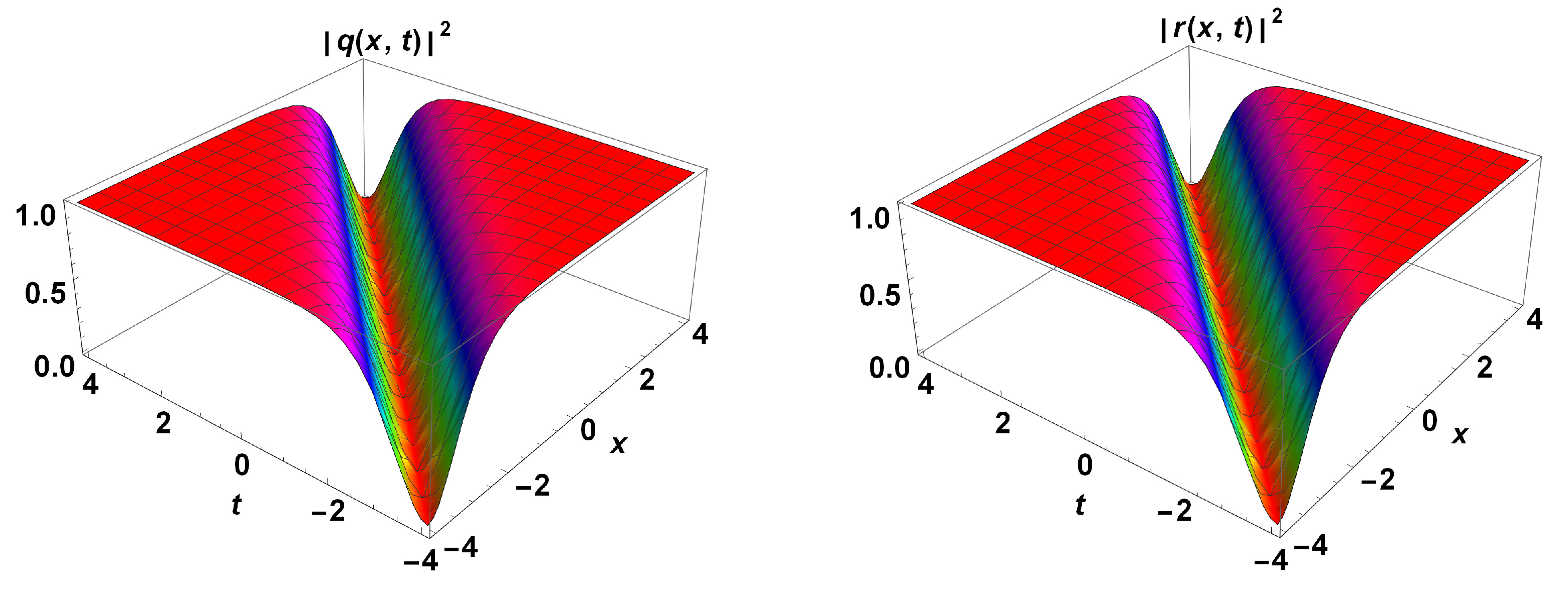
2.2. Dark Solitons

Dark solitons are another type of soliton solution that describes a self-reinforcing wave with a minimum amplitude at its center. They are called “dark” solitons because they appear as a localized dip or dark region in the waveform. Dark soliton solutions arise in many physical systems, including nonlinear optics, Bose–Einstein condensates, and ocean waves. Unlike bright solitons, dark solitons are typically unstable, meaning they eventually break up or decay over long distances. However, they are still of great interest to researchers because of their unique properties and potential applications. For example, they can be used to manipulate and control light in optical systems, and they can provide insight into the behavior of complex systems. The study of dark soliton solutions is an active area of research, with many new models and methods for their analysis and application. Researchers continue to explore the properties of these solutions in various settings, and new discoveries are expected to emerge in the years to come. Dark soliton solutions are an important area of study in modern physics and applied mathematics, with potential applications in a wide range of fields.

The second case to be considered is dark solitons, the wave form assumption ($P_l(x,t)$) of which is

$$\begin{array}{c}\hfill P_l(x,t)=A_l{tanh}^{p_l}\phi ,\phi =B(x-vt).\end{array}$$

(31)

Here, the soliton speed is represented by v, and $A_l$ and B are considered free parameters. The parameter $p_l$ is determined using the principle of balancing. By plugging (31) into (15), we arrive at the simplified expression:

$$\begin{array}{ccc}& & -\{(\omega +a{\kappa }^2+3c_{1l}{\sigma }_{1l}{\kappa }^4)+2p_l^2[(a+6c_{1l}{\sigma }_{1l}{\kappa }^2)-c_{1l}{\sigma }_{1l}(5+3p_l^2)B^2]B^2\}{A}_l{tanh}^{p_l}\phi \hfill \\ & & +\{[b_l-\kappa c_7({\epsilon }_l-{\eta }_l)-c_{1l}{\kappa }^2({\alpha }_l-{\gamma }_l+{\delta }_l+{\mu }_l)]-2p_l^2{c}_{1l}({\alpha }_l+{\gamma }_l+{\delta }_l+{\mu }_l)B^2\}{A}_l^3{tanh}^{3p_l}\phi \hfill \\ & & +f_l{c}_{1l}{A}_l^5{tanh}^{5p_l}\phi +p_l(1+p_l)[(a+6c_{1l}{\sigma }_{1l}{\kappa }^2)-4c_{1l}{\sigma }_{1l}(2+p_l(2+p_l))B^2]A_l{B}^2{tanh}^{2+p_l}\phi \hfill \\ & & +c_{1l}{\sigma }_{1l}{p}_l(1+p_l)(2+p_l)(3+p_l)A_l{B}^4{tanh}^{4+p_l}\phi \hfill \\ & & +p_l[p_l{c}_{1l}({\alpha }_l+{\gamma }_l)+(1+p_l)c_{1l}({\delta }_l+{\mu }_l)]A_l^3{B}^2{tanh}^{2+3p_l}\phi \phantom{pppp}\hfill \\ & & +\{[c_l-\kappa (\kappa c_{1l}({\xi }_l+{\rho }_l-{\lambda }_l)+c_7({\tau }_l-{\theta }_l))]-(p_l^2{c}_{1l}({\xi }_l+{\rho }_l)+{\lambda }_l{p}_{\overline{l}}^2{c}_{1l})B^2\}{A}_l{A}_{\overline{l}}^2{tanh}^{p_l+2p_{\overline{l}}}\phi \hfill \\ & & +h_l{c}_{1l}{A}_l{A}_{\overline{l}}^4{tanh}^{p_l+4p_{\overline{l}}}\phi +g_l{c}_{1l}{A}_l^3{A}_{\overline{l}}^2{tanh}^{3p_l+2p_{\overline{l}}}\phi \hfill \\ & & -p_l(1-p_l)[(a+6c_{1l}{\sigma }_{1l}{\kappa }^2)-4c_{1l}{\sigma }_{1l}(2-p_l(2-p_l))B^2]A_l{B}^2{tanh}^{p_l-2}\phi \hfill \\ & & -p_l(1-p_l)(2-p_l)(3-p_l)c_{1l}{\sigma }_{1l}{A}_l{B}^4{tanh}^{p_l-4}\phi \hfill \\ & & +p_l[p_l{c}_{1l}({\alpha }_l+{\gamma }_l)-(1-p_l)c_{1l}({\delta }_l+{\mu }_l)]A_l^3{B}^2{tanh}^{3p_l-2}\phi \hfill \\ & & +[p_l(p_l-1)c_{1l}({\xi }_l+{\rho }_l)+p_{\overline{l}}^2{\lambda }_l{c}_{1l}]A_l{A}_{\overline{l}}^2{B}^2{tanh}^{p_l+2p_{\overline{l}}-2}\phi \hfill \\ & & +[p_l(1+p_l)c_{1l}({\xi }_l+{\rho }_l)+p_{\overline{l}}^2{\lambda }_l{c}_{1l}]A_l{A}_{\overline{l}}^2{B}^2{tanh}^{p_l+2p_{\overline{l}}+2}\phi =0,\hfill \end{array}$$

(32)

where, as in the previous section, $\overline{l}=3-l$ and $l=1,2$. By inspection, the parameter $p_l$ in this case can be verified to result in (18) for both $l=1$ and $l=2$. Substituting the obtained value of $p_l$ into Equation (32) and setting the coefficients of the functions ${tanh}^j\phi$ with $j=1,3,5$ to zero results in the following expression for the wave number:

$$\omega =-a\left({\kappa }^2+2B^2\right)+c_{1l}\left[\left({\alpha }_l+{\gamma }_l\right)A_l^2+{\lambda }_l{A}_{\overline{l}}^2\right]B^2+c_{1l}{\sigma }_{1l}\left(16B^4-12{\kappa }^2{B}^2-3{\kappa }^4\right),$$

(33)

and the free parameter,

$$\begin{array}{ccc}\hfill B& =& \left[\frac{Z_7-(Z_4+Z_5)A_l^2-(Z_6+c_{1l}{\lambda }_l)A_{\overline{l}}^2}{40c_{1l}{\sigma }_{1l}}\right.\hfill \\ & \pm & {\left.\frac{\sqrt{{[(Z_4+Z_5)A_l^2-Z_7+(c_{1l}{\lambda }_l+Z_6)A_{\overline{l}}^2]}^2+40c_{1l}{\sigma }_{1l}(Z_2{A}_l^2+Z_3{A}_{\overline{l}}^2})}{40c_{1l}{\sigma }_{1l}}\right]}^{\frac{1}{2}},\hfill \end{array}$$

(34)

along with the solvability condition,

$$c_{1l}{f}_l{A}_l^4+c_{1l}{h}_l{A}_{\overline{l}}^4+\left[\left(Z_4+2Z_5\right)B^2+c_{1l}{g}_l{A}_{\overline{l}}^2\right]A_l^2+\left(2Z_6+c_{1l}{\lambda }_l\right)A_{\overline{l}}^2{B}^2+24c_{1l}{\sigma }_{1l}{B}^4=0.$$

(35)

For convenience, we adopted the notations previously given on (22)–(28). It is clear from (34) that

$$c_{1l}{\sigma }_{1l}\ne 0,$$

(36)

and that

$${\left[\left(Z_4+Z_5\right)A_l^2-Z_7+\left(c_{1l}{\lambda }_l+Z_6\right)A_{\overline{l}}^2\right]}^2+40c_{1l}{\sigma }_{1l}\left(Z_2{A}_l^2+Z_3{A}_{\overline{l}}^2\right)\ge 0,$$

(37)

along with the fact that the entire radicand on (34) must be positive. Consequently, the solution for the dark soliton in the considered system can be expressed as follows:

$$\begin{array}{c}\hfill q(x,t)=A_{1}tanh\left[B(x-vt)\right]e^{i\left(-\kappa x+\omega t+\Theta \right)},\end{array}$$

(38)

and

$$\begin{array}{c}\hfill r(x,t)=A_{2}tanh\left[B(x-vt)\right]e^{i\left(-\kappa x+\omega t+\Theta \right)}.\end{array}$$

(39)

Above, described the relationship between the respective free parameters, along with the speed (14) and wave number (33), subject to the constraints discussed above. Plots of the dark solitons described by Equations (38) and (39) with $A_1=1$, $A_2=1$, $\kappa =1$, $a=1$, $c_7=1$, ${\sigma }_7=1$, $c_{1l}=1$, ${\sigma }_{1l}=1$, ${\lambda }_l=1$, ${\alpha }_l=1$, ${\gamma }_l=1$, ${\delta }_l=1$, ${\mu }_l=1$, ${\xi }_l=1$, ${\rho }_l=1$, $b_l=1$, ${\epsilon }_l=1$, ${\eta }_l=1$, $c_l=1$, ${\tau }_l=1$, and ${\theta }_l=1$ are demonstrated in Figure 2. Dark solitons are a type of soliton solution that describes a self-reinforcing wave with a minimum amplitude at its center.

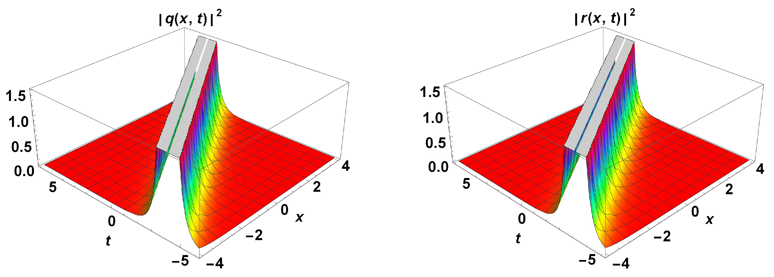
2.3. Singular Solitons

Singular solitons are a type of soliton solution that exhibits a singularity at the center of the wave profile. They are also referred to as peakons because they resemble a peaked function rather than a smooth wave. Singular solitons arise in various fields, including fluid dynamics, nonlinear optics, and plasma physics. Unlike bright and dark solitons, which have a finite energy and amplitude, singular solitons have infinite amplitude at the center of the wave profile. As a result, these solutions are typically highly unstable and cannot propagate over long distances. However, they are still of great interest to researchers because of their unique properties and potential applications. The study of singular soliton solutions is an active area of research, with many new models and methods for their analysis and application. Researchers continue to explore the properties of these solutions in various settings, and new discoveries are expected to emerge in the years to come. Singular soliton solutions are a fascinating and important area of study in modern physics and applied mathematics, with potential applications in fields such as shock wave theory and signal processing.

2.3.1. Singular Solitons (Type I)

In this case, we need to make a certain assumption regarding the waveform, which is:

$$\begin{array}{c}\hfill P_l(x,t)=A_l{csch}^{p_l}\phi ,\phi =B(x-vt).\end{array}$$

(40)

Let us assume that $A_l$ and B are independent variables that are considered as free parameters. By substituting this assumption into (15), we obtain the following result:

$$\begin{array}{ccc}& & \{p_l^2(a+6c_{1l}{\sigma }_{1l}{\kappa }^2)B^2+p_l^4{c}_{1l}{\sigma }_{1l}{B}^4-(\omega +a{\kappa }^2+3c_{1l}{\sigma }_{1l}{\kappa }^4)\}{A}_l{csch}^{p_l}\phi \hfill \\ & & +\{[b_l-\kappa c_7({\epsilon }_l-{\eta }_l)-c_{1l}{\kappa }^2({\alpha }_l-{\gamma }_l+{\delta }_l+{\mu }_l)]+p_l^2{c}_{1l}({\alpha }_l+{\gamma }_l+{\delta }_l+{\mu }_l)B^2\}{A}_l^3{csch}^{3p_l}\phi \hfill \\ & & +f_l{c}_{1l}{A}_l^5{csch}^{5p_l}\phi +p_l(1+p_l)[(a+6c_{1l}{\sigma }_{1l}{\kappa }^2)+2(2+p_l(2+p_l))c_{1l}{\sigma }_{1l}{B}^2]A_l{B}^2{csch}^{2+p_l}\phi \hfill \\ & & +p_l(1+p_l)(2+p_l)(3+p_l)c_{1l}{\sigma }_{1l}{A}_l{B}^4{csch}^{4+p_l}\phi \hfill \\ & & +p_l[p_l{c}_{1l}({\alpha }_l+{\gamma }_l)+(1+p_l)c_{1l}({\delta }_l+{\mu }_l)]A_l^3{B}^2{csch}^{2+3p_l}\phi \hfill \\ & & +\{[c_l-\kappa (\kappa c_{1l}({\xi }_l+{\rho }_l-{\lambda }_l)+c_7({\tau }_l-{\theta }_l))]+(p_{\overline{l}}^2{\lambda }_l{c}_{1l}+p_l^2{c}_{1l}({\xi }_l+{\rho }_l))B^2\}{A}_l{A}_{\overline{l}}^2{csch}^{p_l+2p_{\overline{l}}}\phi \hfill \\ & & +g_l{c}_{1l}{A}_l^3{A}_{\overline{l}}^2{csch}^{3p_l+2p_{\overline{l}}}\phi +h_l{c}_{1l}{A}_l{A}_{\overline{l}}^4{csch}^{p_l+4p_{\overline{l}}}\phi \hfill \\ & & +[p_{\overline{l}}^2{\lambda }_l{c}_{1l}+p_l(1+p_l)c_{1l}({\xi }_l+{\rho }_l)]A_l{A}_{\overline{l}}^2{B}^2{csch}^{2+p_l+2p_{\overline{l}}}\phi =0,\hfill \end{array}$$

(41)

after simplification, where $\overline{l}=3-l$ and $l=1,2.$ Balancing the cubic nonlinearity and second-order dispersion in the final equation results in the determination of $p_l$ as presented in Equation (18). We then substitute the obtained value of $p_l$ and, following the same procedure as for dark and bright solitons, gather the coefficients of ${csch}^j\phi$ for $j=1,3,5$, which results in the same wave number as that of the dark soliton solution given by Equation (19). The free parameter (B) is also determined by

$$\begin{array}{ccc}\hfill B& =& \left[\frac{-(Z_4+Z_5)A_l^2-Z_7-(c_{1l}{\lambda }_l+Z_6)A_{\overline{l}}^2}{40c_{1l}{\sigma }_{1l}}\right.\hfill \\ & \pm & {\left.\pm \frac{\sqrt{{[(Z_4+Z_5)A_l^2+2Z_7+(c_{1l}{\lambda }_l+Z_6)A_{\overline{l}}^2]}^2-80c_{1l}{\sigma }_{1l}(Z_2{A}_l^2+Z_3{A}_{\overline{l}}^2})}{40c_{1l}{\sigma }_{1l}}\right]}^{\frac{1}{2}},\hfill \end{array}$$

(42)

while the identity equation is the same as in the dark soliton case (35). Here, we again adopted the expressions given in (22)–(28). Clearly, the constraint (36) also applies here, and (37) slightly changes to

$${\left[\left(Z_4+Z_5\right)A_l^2+2Z_7+\left(c_{1l}{\lambda }_l+Z_6\right)A_{\overline{l}}^2\right]}^2-80c_{1l}{\sigma }_{1l}\left(Z_2{A}_l^2+Z_3{A}_{\overline{l}}^2\right)\ge 0.$$

(43)

As a result, the singular soliton solutions for the system described by Equations (2) and (3) are introduced as below

$$\begin{array}{c}\hfill q(x,t)=A_{1}csch\left[B(x-vt)\right]e^{i\left(-\kappa x+\omega t+\Theta \right)},\end{array}$$

(44)

and

$$\begin{array}{c}\hfill r(x,t)=A_{2}csch\left[B(x-vt)\right]e^{i\left(-\kappa x+\omega t+\Theta \right)}.\end{array}$$

(45)

As previously discussed, the relevant parameters and their corresponding constraints have been outlined above. Plots of the singular solitons described by Equations (44) and (45) with $A_1=1$, $A_2=1$, $\kappa =1$, $a=1$, $c_7=1$, ${\sigma }_7=1$, $c_{1l}=1$, ${\sigma }_{1l}=1$, ${\lambda }_l=1$, ${\alpha }_l=1$, ${\gamma }_l=1$, ${\delta }_l=1$, ${\mu }_l=1$, ${\xi }_l=1$, ${\rho }_l=1$, $b_l=1$, ${\epsilon }_l=1$, ${\eta }_l=1$, $c_l=1$, ${\tau }_l=1$, and ${\theta }_l=1$ are depicted in Figure 3. Singular solitons are a type of soliton solution that exhibits a singularity at the center of the wave profile.

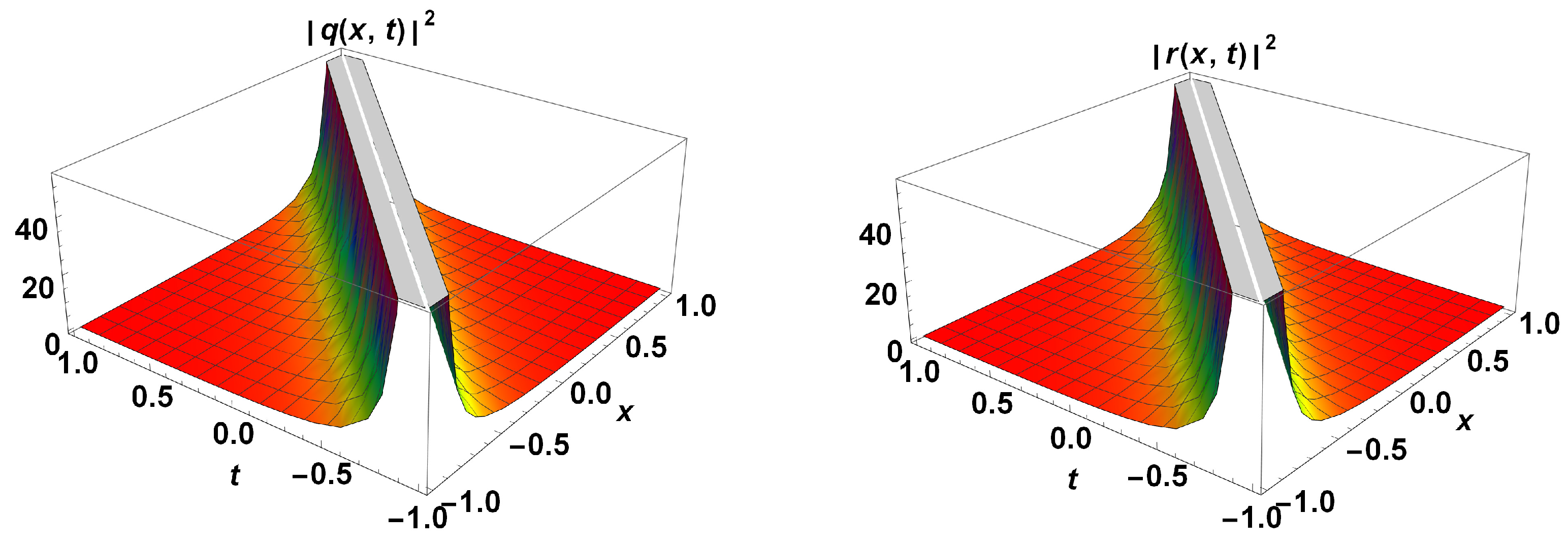
2.3.2. Singular Solitons (Type II)

In this case, the assumption for the waveform portion ($P_l(x,t)$) is

$$\begin{array}{c}\hfill P_l(x,t)=A_l{coth}^{p_l}\phi ,\phi =B(x-vt).\end{array}$$

(46)

Similarly, the parameters $A_l$ and B are considered to be free parameters. Substituting them into Equation (15) yields the following relation

$$\begin{array}{ccc}\hfill & & -\{(\omega +a{\kappa }^2+3c_{1l}{\sigma }_{1l}{\kappa }^4)+2p_l^2[(a+6c_{1l}{\sigma }_{1l}{\kappa }^2)-(5+3p_l^2)B^2]B^2\}{A}_l{coth}^{p_l}\phi \hfill \\ & & +\{[b_l-\kappa c_7({\epsilon }_l-{\eta }_l)-c_{1l}{\kappa }^2({\alpha }_l-{\gamma }_l+{\delta }_l+{\mu }_l)]-2p_l^2{c}_{1l}({\alpha }_l+{\gamma }_l+{\delta }_l+{\mu }_l)B^2\}{A}_l^3{coth}^{3p_l}\phi \hfill \\ & & +p_l(1+p_l)[(a+6c_{1l}{\sigma }_{1l}{\kappa }^2)-4(2+p_l(2+p_l))c_{1l}{\sigma }_{1l}{B}^2]A_l{B}^2{coth}^{2+p_l}\phi \hfill \\ & & +f_l{c}_{1l}{A}_l^5{coth}^{5p_l}\phi +p_l(1+p_l)(2+p_l)(3+p_l)c_{1l}{\sigma }_{1l}{A}_l{B}^4{coth}^{4+p_l}\phi \hfill \\ & & +p_l[p_l{c}_{1l}({\alpha }_l+{\gamma }_l)+(1+p_l)c_{1l}({\delta }_l+{\mu }_l)]A_l^3{B}^2{coth}^{2+3p_l}\phi \hfill \\ & & -p_l(1-p_l)[(a+6c_{1l}{\sigma }_{1l}{\kappa }^2)-4(2-p_l(2-p_l))c_{1l}{\sigma }_{1l}{B}^2]A_l{B}^2{coth}^{-2+p_l}\phi \hfill \\ & & -p_l(1-p_l)(2-p_l)(3-p_l)c_{1l}{\sigma }_{1l}{A}_l{B}^4{coth}^{-4+p_l}\phi \hfill \\ & & +p_l[p_l{c}_{1l}({\alpha }_l+{\gamma }_l)-(1-p_l)c_{1l}({\delta }_l+{\mu }_l)]A_l^3{B}^2{coth}^{-2+3p_l}\phi \hfill \\ & & +h_l{c}_{1l}{A}_l{A}_{\overline{l}}^4{coth}^{p_l+4p_{\overline{l}}}\phi +g_l{c}_{1l}{A}_l^3{A}_{\overline{l}}^2{coth}^{3p_l+2p_{\overline{l}}}\phi \hfill \\ & & +[p_{\overline{l}}^2{\lambda }_l{c}_{1l}+p_l(1+p_l)c_{1l}({\xi }_l+{\rho }_l)]A_l{A}_{\overline{l}}^2{B}^2{coth}^{2+p_l+2p_{\overline{l}}}\phi \hfill \\ & & +[p_{\overline{l}}^2{\lambda }_l{c}_{1l}-p_l(1-p_l)c_{1l}({\xi }_l+{\rho }_l)]A_l{A}_{\overline{l}}^2{B}^2{coth}^{-2+p_l+2p_{\overline{l}}}\phi \hfill \\ & & +\{[c_l-\kappa (\kappa c_{1l}({\xi }_l+{\rho }_l-{\lambda }_l)+c_7({\tau }_l-{\theta }_l))]-2[p_{\overline{l}}^2{\lambda }_l{c}_{1l}+p_l^2{c}_{1l}({\xi }_l+{\rho }_l)]B^2\}{A}_l{A}_{\overline{l}}^2{coth}^{p_l+2p_{\overline{l}}}\phi =0.\hfill \end{array}$$

(47)

In this case, the balancing algorithm and coefficients of the standalone elements, specifically ${coth}^{-2+p_l}\phi$ and ${coth}^{-4+p_l}\phi$, provide us the value of $p_l$ as presented in Equation (18). Upon substituting the obtained value of $p_l$ from Equation (18) into Equation (47), the resulting solutions and corresponding solvability conditions are identical to those obtained for the case of a dark soliton, as shown in Equations (33)–(37). Consequently, the concatenation coupled model given by Equations (2) and (3) possesses type-II singular soliton solutions, which are introduced below

$$\begin{array}{c}\hfill q(x,t)=A_{1}coth\left[B(x-vt)\right]e^{i\left(-\kappa x+\omega t+\Theta \right)},\end{array}$$

(48)

and

$$\begin{array}{c}\hfill r(x,t)=A_{2}coth\left[B(x-vt)\right]e^{i\left(-\kappa x+\omega t+\Theta \right)},\end{array}$$

(49)

where all the relevant parameters and their corresponding constraints for these solitons are identical to those for dark solitons. Plots of the singular solitons described by Equations (48) and (49) with $A_1=1$, $A_2=1$, $\kappa =1$, $a=1$, $c_7=1$, ${\sigma }_7=1$, $c_{1l}=1$, ${\sigma }_{1l}=1$, ${\lambda }_l=1$, ${\alpha }_l=1$, ${\gamma }_l=1$, ${\delta }_l=1$, ${\mu }_l=1$, ${\xi }_l=1$, ${\rho }_l=1$, $b_l=1$, ${\epsilon }_l=1$, ${\eta }_l=1$, $c_l=1$, ${\tau }_l=1$, and ${\theta }_l=1$ are presented in Figure 4. Soliton solutions that display a singularity at the center of the wave profile are referred to as singular solitons.

3. Conclusions

In the current, we paper addressed optical solitons in a birefringent fiber modeled by the concatenation-type governing equation. Three standard equations are concatenated to formulate the model. They are the most familiar NLSE, the LPD model, and the SSE. The model of study was integrated using the principle of undetermined coefficients. This resulted in the retrieval of bright, dark, and singular (both kinds) one-soliton solutions to the model, along with the applicable constraint conditions that naturally emerged during the course of the derivation of the soliton solution.

While this is a simple approach, it has its merits and shortcomings. It is simple in the sense that after picking an appropriate hypothesis and inserting it into the equation, the parameter relations and constraints naturally emerge. The imaginary part relation gives the soliton velocity and additional constraint relations that must remain valid for the solitons to exist. One of the shortcomings is that it fails to recover multisoliton solutions, unlike inverse scattering transform (IST) or the Hirota’s bilinear approach. Another disadvantage is it is unable to go past the discrete regime and provide an answer for the continuous regime. In other words, the algorithm does not yield soliton radiation. In order to recover soliton radiation, one must implement additional approaches such as IST or, beyond all order asymptotics, even applying the theory of unfoldings. Another disadvantage is that the method fails to obtain additional soliton solutions such as the straddled solitons. However, these can be recovered with the aid of Kudryashov’s approach.

With the fundamental results in place, various avenues are opened, presenting opportunities for future studies. First, an immediate burning question would be, “What are the conservation laws?”. Such laws will be investigated in a separate paper, with conserved densities derived using the multipliers approach and listed after computing the conserved quantities from the bright one-soliton solution derived in this paper.

The model proposed in this paper involves differential group delay, while in a previous report, the same model was investigated but for the scalar case [3]. Dispersion-flattened fibers can be explored in future work. This would provide a newer perspective to extract the soliton solutions and provide a new perspective of possible conservation laws.

The inclusion of perturbation terms is our next target. Thus, the perturbed concatenation model will be analyzed for its integrability. The availability of conservation laws would mean that one can compute the adiabatic parameter dynamics of the soliton parameters via the soliton perturbation theory. One can also implement the moment method or the collective variables approach to recover this kind of dynamical system.

The integrability of the perturbed model also needs to be studied to recover the soliton solution when the concatenation model includes perturbation terms. This depends on two situations. If the perturbation terms are weak, with quasimonochromaticity, one must integrate the perturbed concatenation model approximately with the use of multiscale perturbation analysis, irrespective of the type of perturbation term, be it Hamiltonian or non-Hamiltonian. Thus, a quasistationary soliton solution would be revealed, along with the resonance conditions. However, if the perturbation terms are strong but of Hamiltonian type, several integration schemes are available to integrate the perturbed concatenation model. A few such schemes are Kudryashov’s approach, Jacobi’s elliptic function scheme, and the sin-Gordon equation scheme, just to mention a few. In the final situation, when the perturbation terms are strong but non-Hamiltonian type, a slick scheme needs to be implemented that considers the model with time-dependent coefficients and applies an integration scheme possibly including the method of undetermined coefficients. This would naturally apply constraints on the parameter and the time-dependent coefficients. Some of the non-Hamiltonian perturbations to which this scheme can be successfully applied are the linear attenuation effect and Raman scattering, among others. All of these possibilities are subject to one exception. If the perturbation term(s) contain(s) maximum intensity, all of the above-mentioned integration approaches fail miserably. In that case, one must resort to approximate integration with the aid of the semi-inverse variational principle. In this case, it is only the bright one-soliton solution that can be recovered, and the retrieval of dark or singular solitons is not possible because the stationary integral is rendered divergent.

With adiabatic parameter dynamics in place, which can be recovered with the use of soliton perturbation theory, one can address the suppression of intrachannel collision of solitons with the aid of quasiparticle theory, which is yet to be developed for the concatenation model.

Then, the application of the model to additional devices apart from optical fibers can be considered. This would involve the implementation of the model for magneto-optic wave guides, Bragg grating fibers, and optical couplers, as well as for the study the concatenation model in optical metamaterials. Thus, gap solitons and magneto-optic solitons would be subsequently recovered and reported. Moreover, the governing model should addressed with fractional temporal evolution rather than linear temporal evolution as in the current paper and most previous papers. The consideration of fractional temporal evolution would lead to the slow evolution of solitons, meaning that one can successfully control the Internet bottleneck effect, which is a growing problem in the telecommunication industry. Another viable approach to this problem is to introduce the spatiotemporal dispersion (STD), in addition to pre-existing chromatic dispersion (CD). This combination if CD and STD can also be used as an engineering marvel to mitigate the Internet bottleneck effect.

One of the viable aspects to further consider with respect to this concatenation model is the nonlinearity of the CD. This can occur due to rough handling of fibers, as well as the random injection of pulses at the initial end of the fiber. When the CD becomes nonlinear, soliton transmission across intercontinental distance is stalled, and this leads to the formation of quiescent solitons—a very unwanted feature. While this aspect has already been studied for the scalar case, it must be addressed for fibers with differential group delay and dispersion-flattened fibers.

Apart from the various considerations for the analytical approaches listed thus far, one must additionally consider a model with the use of numerical algorithms. Some of the most applicable numerical schemes are the Adomian decomposition method, the improved Adomian decomposition approach, the Laplace–Adomian decomposition scheme, and the variational iteration method. Several other numerical algorithms that can be implemented to address the problem include the finite difference method, the finite element method, the finite volume scheme, and spectral approaches [8,9,10,11,12,13,14,15,16,17,18,19,20,21,22,23,24,25,26,27,28,29,30,31,32,33,34,35]. Thus, much work remains to be done in this field.