Optimal Model Averaging Estimation for the Varying-Coefficient Partially Linear Models with Missing Responses

Abstract

In this paper, we propose a model averaging estimation for the varying-coefficient partially linear models with missing responses. Within this context, we construct a HR$C_p$ weight choice criterion that exhibits asymptotic optimality under certain assumptions. Our model averaging procedure can simultaneously address the uncertainty on which covariates to include and the uncertainty on whether a covariate should enter the linear or nonlinear component of the model. The simulation results in comparison with some related strategies strongly favor our proposal. A real dataset is analyzed to illustrate the practical application as well.

1. Introduction

Model averaging, an alternative to model selection, addresses both model uncertainty and estimation uncertainty by appropriately compromising over the set of candidate models, instead of picking only one of them, and this generally leads to much smaller risk than that encountered in model selection. Over the past decade, various model averaging approaches, with optimal large sample properties have been actively proposed for complete data setting, such as the following: Mallows model averaging [1,2], optimal mean squared error averaging [3], jackknife model averaging [4,5,6], heteroscedasticity-robust $C_p$ (HR$C_p$) model averaging [7], model averaging based on Kullback–Leibler distance [8], model averaging in a kernel regression setup [9], and model averaging based on K-fold cross-validation [10], among others.

In practice, many datasets in clinical trials, opinion polls and market research surveys often contain missing values. As far as we know, compared with the large body of research regarding model averaging for fully observed data, much less attention has been paid to performing optimal model averaging in the presence of missing data. Reference [11] studied a model averaging method applicable to situations in which covariates are missing completely at random, by adapting a Mallows criterion based on the data from complete cases. Reference [12] broadened the analysis in [11] to a fragmentary data and heteroscedasticity setup. By applying the HR$C_p$ approach in [7], Reference [13] developed an optimal model averaging method in the presence of responses missing at random (MAR). In the context of missing response data, Reference [14] constructed a model averaging method based on a delete-one cross-validation criterion. Reference [15] proposed a two-step model averaging procedure for high-dimensional regression with missing responses at random.

The aforementioned model averaging methods in a missing data setting are asymptotically optimal in the sense of minimizing the squared error loss in a large sample case, but they all concentrate mainly on the simple linear regression model. In the context of missing data, it would be interesting to study model averaging in the varying-coefficient partially linear model (VCPLM) introduced by [16], which allows interactions between a covariate and an unknown function through effect modifiers. Due to its flexible specification and explanatory power, this model has received extensive attention over the past decades. Different kinds of approaches have been raised to estimate the VCPLM, such as the following: estimation process based on the local polynomial fitting method [17], the general series method [18], and profile least squares estimation [19]. References [20,21,22,23] have developed various variable selection procedures in the VCPLM. As for model averaging in the VCPLM, only the following works have been conducted. In the measurement error model and the missing data model, References [24,25], respectively, established the limiting distribution of the resulting model averaging estimators of the unknown parameters of interest under the local misspecification framework. As pointed out by [26], this framework, which was suggested by [27], is a useful tool for asymptotic analysis, but its realism is subject to considerable criticism. Additionally, these two works studied existing model averaging strategies, based on the focused information criterion, but did not consider any new model averaging method with asymptotic optimality. When all data are available, References [26,28] developed two asymptotically optimal model averaging approaches for the VCPLM, based on a Mallows-type criterion and a jackknife criterion, respectively.

As far as we know, there remains no optimal model averaging approach developed for the VCPLM with missing responses. The main goal of the current paper was to fill this gap. To the best of our knowledge, this paper is the first to study the asymptotically optimal model averaging approach for the VCPLM in the presence of responses MAR without the local misspecification assumption. However, existing results are difficult to directly extend to our setup for the following two reasons. Firstly, existing optimal model averaging approaches in the VCPLM with complete data, such as the Mallows model averaging method proposed by [26], and the jackknife model averaging method advocated by [28], cannot be directly applied to our problem. Secondly, in contrast with the case in linear missing data models, studied by [13,14], our analysis is significantly complicated by two kinds of uncertainty in the VCPLM: the uncertainty on the selection of variables, and the uncertainty on whether a covariate should be allocated to the linear or nonlinear component of the model. These uncertainties have not been investigated much by the VCPLM literature. Motivated by these two challenges, we suggest a new model averaging approach for the VCPLM with responses MAR via the HR$C_p$ criterion. This new approach was developed by introducing a synthetic response based on an inverse probability weighted (IPW) technique. Then, HR$C_p$ model averaging could be conducted easily. Under certain assumptions, the weights selected by minimizing the HR$C_p$ criterion are demonstrated to be asymptotically optimal. Furthermore, we numerically illustrate that our method is always superior to its rivals in several designs with different kinds of model uncertainty. The detailed research procedures and methods can be found in Figure 1.

The remainder of this article is organized as follows. We construct the model averaging estimator and establish its asymptotic optimality in Section 2. A simulation study is conducted in Section 3 to illustrate the finite sample performance of our strategy and a real data example is provided in Section 4. Section 5 contains some conclusions. Detailed proofs of the main results are relegated to the Appendix A.

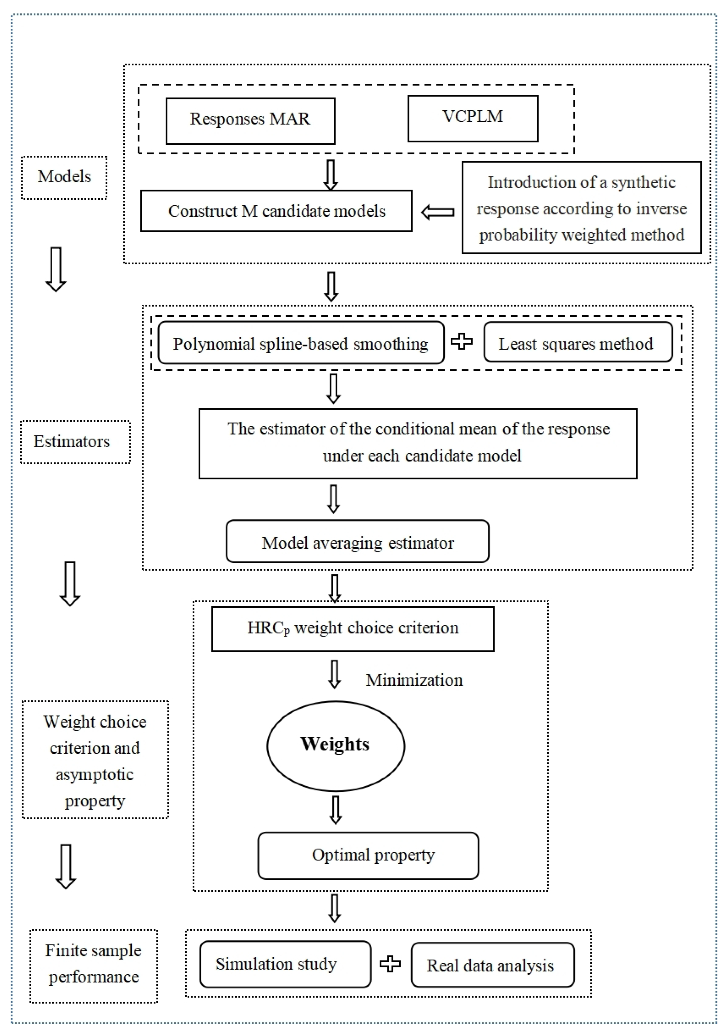
2. Model Averaging Estimation

2.1. Model and Estimators

We considered the following VCPLM:

$$y_i={\mu }_i+{ϵ}_i=X_i^{\prime }\beta +Z_i^{\prime }\alpha (u_i)+{ϵ}_i=\sum _{p=1}^{\infty }{x}_{ip}{\beta }_p+\sum _{q=1}^{\infty }{z}_{iq}{\alpha }_q(u_i)+{ϵ}_i,i=1,\dots ,n,$$

(1)

where $y_i$ is a scalar response variable, $(X_i,Z_i,u_i)$ are covariates with $X_i$ and $Z_i$ being countably infinite, $\beta$ is an unknown coefficient vector associated with $X_i$, $\alpha (·)$ is an unknown coefficient function vector associated with $Z_i$, ${ϵ}_i$ is a random statistical error with $E({ϵ}_i|X_i,Z_i,u_i)=0$ and $E({ϵ}_i^2|X_i,Z_i,u_i)={\sigma }^2$. As in [26,29], we assume that the dimension of $u_i$ is one. Model (1) is flexible enough to cover a variety of other existing models, such as the following: the linear model that was studied by [1,4], the partially linear model that was studied by [30] and the varying-coefficient model that was studied by [29]. For this model, we focus on the case where all covariates are always fully observed while some observations of the response variable may be missing. Specifically, we assume that $y_i$ is MAR in the sense that:

$$P({\delta }_i=1|y_i,X_i,Z_i,u_i)=P({\delta }_i=1|X_i,Z_i,u_i)\equiv \pi (X_i,Z_i,u_i),$$

(2)

where ${\delta }_i=1$ if $y_i$ is completely observed, otherwise ${\delta }_i=0$, and the selection probability function $\pi (X_i,Z_i,u_i)$ is bounded away from 0.

As in most literature on model averaging, we aimed to estimate the conditional mean of the response data $Y={(y_1,\dots ,y_n)}^{\prime }$, i.e., $\mu ={({\mu }_1,\dots ,{\mu }_n)}^{\prime }$, which is especially useful in prediction. However, owing to the presence of the missing data, none of the existing optimal model averaging estimations for complete data could be directly utilized in our setting. We addressed this problem by introducing a synthetic response $H_{\pi ,i}={\delta }_i{y}_i/\pi (X_i,Z_i,u_i)$. By the aforementioned MAR assumption and some simple calculations, it is easy to observe that $E(H_{\pi ,i}|X_i,Z_i,u_i)=E(y_i|X_i,Z_i,u_i)={\mu }_i$ and $\mathrm{Var}(H_{\pi ,i}|X_i,Z_i,u_i)={\sigma }_{\pi ,i}^2$, where ${\sigma }_{\pi ,i}^2=\left[{\{\pi (X_i,Z_i,u_i)\}}^{-1}-1\right]{\mu }_i^2+{\{\pi (X_i,Z_i,u_i)\}}^{-1}{\sigma }^2$. Therefore, under Model (1) and the MAR assumption, we have:

$$H_{\pi ,i}={\mu }_i+{ϵ}_{\pi ,i},i=1,\dots ,n,$$

(3)

where ${ϵ}_{\pi ,i}=H_{\pi ,i}-E(y_i|X_i,Z_i,u_i)$ satisfying $E({ϵ}_{\pi ,i}|X_i,Z_i,u_i)=0$ and $\mathrm{Var}({ϵ}_{\pi ,i}|X_i,Z_i,u_i)={\sigma }_{\pi ,i}^2$. As is apparent, in Model (3) the completely observed cases are weighted by their corresponding inverse selection probabilities, while the missing cases are weighted by zeros. Then, the analysis is conducted on the basis of the weighted data. By introducing the fully observed synthetic response $H_{\pi ,i}$, we obtain a new Model (3) the conditional expectation of which is equivalent to that of Model (1). Thus, the HR$C_p$ model averaging estimation for ${\mu }_i$, the conditional mean of Model (1), can be alternatively derived by studying the HR$C_p$ model averaging estimation for Model (3) with the synthetic data when $\pi (X_i,Z_i,u_i)$ is known.

Supposing that there are M candidate VCPLMs to approximate the true data generating process of $y_i$, which is given in (1), and the mth candidate VCPLM comprises $p_m$ covariates in $X_i$ and $q_m$ covariates in $Z_i$. Accordingly, there are M candidate models to approximate Model (3), and the mth candidate model contains the same covariates as that of the mth candidate VCPLM for (1). Specifically, the mth candidate model is:

$$H_{\pi ,i}=X_{(m),i}^{\prime }{\beta }_{(m)}+Z_{(m),i}^{\prime }{\alpha }_{(m)}(u_i)+e_{(m),i}+{ϵ}_{\pi ,i},i=1,\dots ,n,$$

(4)

where $X_{(m),i}$ is the $p_m$-dimensional sub-vector of $X_i$ and ${\beta }_{(m)}$ is the corresponding unknown coefficient vector, $Z_{(m),i}={(z_{(m),i1},\dots ,z_{(m),i{q}_m})}^{\prime }$ is the $q_m$-dimensional sub-vector of $Z_i$ and ${\alpha }_{(m)}(u_i)={({\alpha }_{(m),1}(u_i),\dots ,{\alpha }_{(m),q_m}(u_i))}^{\prime }$ is the corresponding unknown coefficient function, $e_{(m),i}={\mu }_i-X_{(m),i}^{\prime }{\beta }_{(m)}-Z_{(m),i}^{\prime }{\alpha }_{(m)}(u_i)$ denotes the approximation error of the mth candidate model. Details of the model averaging estimation procedure in our setup are provided below.

We employed the polynomial spline-based smoothing strategy to estimate each coefficient function first. Without loss of generality, suppose that the covariate u is distributed on a compact interval $[0,1]$. Denote the polynomial spline space of degree $\varrho$ on interval $[0,1]$ by $\mathsf{\Psi }$. We introduce a sequence of knots on the interval $[0,1]$: $k_{-\varrho }=\cdots =k_{-1}=k_0=0<k_1<\cdots <k_{J_n}<1=k_{J_n+1}=\cdots =k_{J_n+\varrho +1}$, where the number of interior knots $J_n$ increases with sample size n. The spline basis functions are polynomials of degree $\varrho$ on all sub-intervals $[k_j,k_{j+1})$, $j=0,\dots ,J_n-1$ and $[k_{J_n},1]$, and are $(\varrho -1)$-times continuously differentiable on $[0,1]$. Let $B(·)={(B_{-\varrho }(·),\dots ,B_{J_n}(·))}^{\prime }$ be a vector of the B-spline basis function in space $\mathsf{\Psi }$. According to B-spline theory, there exists a $B^{\prime }(u){\theta }_{(m),q}$ in $\mathsf{\Psi }$ for some $(J_n+\varrho +1)$-dimensional spline coefficient vector ${\theta }_{(m),q}={({\theta }_{(m),q,-\varrho },\dots ,{\theta }_{(m),q,J_n})}^{\prime }$ such that ${max}_{m,q}{sup}_{u\in [0,1]}|{\alpha }_{(m),q}(u)-B^{\prime }(u){\theta }_{(m),q}|=O({(J_n+\varrho +1)}^{-d})$, where ${\alpha }_{(m),q}(u)$ is the qth element of ${\alpha }_{(m)}(u)$. We would like to estimate ${\beta }_{(m)}$ and ${\theta }_{(m)}={({\theta }_{(m),1}^{\prime },\dots ,{\theta }_{(m),q_m}^{\prime })}^{\prime }$ by the least squares method based on the criterion:

$${\displaystyle \underset{{\beta }_{(m)},{\theta }_{(m)}}{min}\sum _{i=1}^n{\left\{{\displaystyle H_{\pi ,i}-X_{(m),i}^{\prime }{\beta }_{(m)}-\sum _{q=1}^{q_m}{z}_{(m),iq}{B}^{\prime }(u_i){\theta }_{(m),q}}\right\}}^2.}$$

(5)

Let $G_{(m),i}={(z_{(m),i1}{B}^{\prime }(u_i),\dots ,z_{(m),i{q}_m}{B}^{\prime }(u_i))}^{\prime }$ be an $\{q_m(J_n+\varrho +1)\}$-dimensional vector. Denote $H_{\pi }={(H_{\pi ,1},\dots ,H_{\pi ,n})}^{\prime }$, $X_{(m)}={(X_{(m),1},\dots ,X_{(m),n})}^{\prime }$ and $G_{(m)}=(G_{(m),1},\dots ,$$G_{(m),n}{)}^{\prime }$. Here, we assume that the regressor matrix ${\tilde{X}}_{(m)}=(X_{(m)},G_{(m)})$ has full column rank $l_m=p_m+\{q_m(J_n+\varrho +1)\}$. The solution to the minimization problem provided in (5) can be expressed as:

$${\widehat{\beta }}_{(m,\pi )}={\{X_{(m)}^{\prime }(I-Q_{(m)})X_{(m)}\}}^{-1}{X}_{(m)}^{\prime }(I-Q_{(m)})H_{\pi },$$

(6)

$${\widehat{\theta }}_{(m,\pi )}={(G_{(m)}^{\prime }{G}_{(m)})}^{-1}{G}_{(m)}^{\prime }(H_{\pi }-X_{(m)}{\widehat{\beta }}_{(m,\pi )}),$$

(7)

where $Q_{(m)}=G_{(m)}{(G_{(m)}^{\prime }{G}_{(m)})}^{-1}{G}_{(m)}^{\prime }$. Let ${\mathsf{\Phi }}_{(m)}=(I-Q_{(m)})X_{(m)}$, then the estimator of $\mu$ under the mth candidate model follows:

$${\widehat{\mu }}_{(m,\pi )}=X_{(m)}{\widehat{\beta }}_{(m,\pi )}+G_{(m)}{\widehat{\theta }}_{(m,\pi )}=\{Q_{(m)}+{\mathsf{\Phi }}_{(m)}{({\mathsf{\Phi }}_{(m)}^{\prime }{\mathsf{\Phi }}_{(m)})}^{-1}{\mathsf{\Phi }}_{(m)}^{\prime }\}{H}_{\pi }.$$

(8)

Denoting $P_{(m)}=Q_{(m)}+{\mathsf{\Phi }}_{(m)}{({\mathsf{\Phi }}_{(m)}^{\prime }{\mathsf{\Phi }}_{(m)})}^{-1}{\mathsf{\Phi }}_{(m)}^{\prime }$, we obtain ${\widehat{\mu }}_{(m,\pi )}=P_{(m)}{H}_{\pi }$.

To smooth estimators across all candidate models, we may define the model averaging estimator of $\mu$ as:

$${\displaystyle {\widehat{\mu }}_{\pi }(w)=\sum _{m=1}^M{w}_m{\widehat{\mu }}_{(m,\pi )}=\sum _{m=1}^M{w}_m{P}_{(m)}{H}_{\pi }\equiv P(w)H_{\pi },}$$

(9)

where $w={(w_1,\dots ,w_M)}^{\prime }$ is a weight vector in the set $\mathcal{W}=\{w\in {[0,1]}^M:{\sum }_{m=1}^M{w}_m=1\}$.

2.2. Weight Choice Criterion and Asymptotically Optimal Property

Obviously, the weight vector w, which represents the contribution of each candidate model in the final estimation, plays a central role in (9). Our weight choice criterion was motivated by applying the HR$C_p$ method of [7], which is designed for the complete data setting, and is defined as follows:

$${\displaystyle C_{\pi }(w)={\parallel H_{\pi }-{\widehat{\mu }}_{\pi }(w)\parallel }^2+2\sum _{i=1}^n{\widehat{ϵ}}_{\pi ,i}^2{P}_{ii}(w),}$$

(10)

where ${\widehat{ϵ}}_{\pi ,i}$ is the residual from a preliminary estimation, $P_{ii}(w)$ is the ith diagonal element of the matrix $P(w)$. As suggested by [7], ${\widehat{ϵ}}_{\pi ,i}$ can be obtained by a model, indexed by $M^{*}$, which includes all the regressors in the candidate models. That is:

$${\widehat{ϵ}}_{\pi }=\sqrt{n/(n-l_{M^{*}})}(I-P_{M^{*}})H_{\pi },$$

(11)

where $l_{M^{*}}$ is the rank of the regressor matrix in model $M^{*}$, ${\widehat{ϵ}}_{\pi }={({\widehat{ϵ}}_{\pi ,1},\dots ,{\widehat{ϵ}}_{\pi ,n})}^{\prime }$.

So far, we have assumed that the selection probability function is known. This is, of course, not the case in real-world data analysis, and the proposed criterion (10) is, hence, computationally infeasible. To obtain a feasible criterion in practice, we needed to estimate $\pi (X_i,Z_i,u_i)$ first. Following much of the missing data literature, and under the MAR assumption defined above, we assume that for an unknown parameter vector $\eta$ and $T_i={(X_i^{\prime },Z_i^{\prime },u_i)}^{\prime }$ we have:

$$\pi (X_i,Z_i,u_i)=\pi (T_i,\eta ),$$

(12)

for some function $\pi (·,\eta )$, the form which is known to be a finite-dimensional parameter $\eta$. Let $\widehat{\eta }$ be the maximum likelihood estimator (MLE) of $\eta$. Then the selection probability function can be estimated by $\pi (T_i,\widehat{\eta })$. In what follows, the Greek letter indexed by $\widehat{\pi }$ denotes that it is obtained by replacing $\pi (X_i,Z_i,u_i)$ in its equation with the estimator $\pi (T_i,\widehat{\eta })$. A feasible form of the weight choice criterion based on HR$C_p$ method is, thus, given by:

$${\displaystyle C_{\widehat{\pi }}(w)={\parallel H_{\widehat{\pi }}-{\widehat{\mu }}_{\widehat{\pi }}(w)\parallel }^2+2\sum _{i=1}^n{\widehat{ϵ}}_{\widehat{\pi },i}^2{P}_{ii}(w),}$$

(13)

and the weight vector can be obtained by:

$$\widehat{w}=arg\underset{w\in \mathcal{W}}{min}{C}_{\widehat{\pi }}(w).$$

(14)

Then, the corresponding model averaging estimator of $\mu$ can be expressed as ${\widehat{\mu }}_{\widehat{\pi }}(\widehat{w})$, and its asymptotic optimality can be developed under some regularity conditions.

Some notations and definitions are required before we list these conditions. Write $l(\eta )=E\left[\delta log\pi (T,\eta )+(1-\delta )log\{1-\pi (T,\eta )\}\right]$, $X={(X_1,\dots ,X_n)}^{\prime }$, $Z={(Z_1,\dots ,Z_n)}^{\prime }$, $U={(u_1,\dots ,u_n)}^{\prime }$. Define the squared error loss of ${\widehat{\mu }}_{\pi }(w)$ and the corresponding risk as $L_{\pi }(w)={\parallel {\widehat{\mu }}_{\pi }(w)-\mu \parallel }^2$ and $R_{\pi }(w)=E(L_{\pi }(w)|X,Z,U)$. Let ${\xi }_{\pi }={inf}_{w\in \mathcal{W}}{R}_{\pi }(w)$, $w_m^0$ be a $M\times 1$ vector with the mth element being 1 and the others being 0, and let ${\mathsf{\Theta }}_{\eta }$ be the parameter space of $\eta$. Define r as a positive integer and $\tau \in (0,1]$, such that $d=(r+\tau )>0.5$. Let $\mathcal{S}$ be a collection of functions s on $[0,1]$ whose rth derivative $s^{(r)}$ exists and satisfies the Lipschitz condition of order $\tau$, i.e.,

$$|s^{(r)}(t^{*})-s^{(r)}(t)|\le C_s{|t^{*}-t|}^{\tau },\mathrm{for}0\le t^{*},t\le 1,$$

where $C_s$ is a positive constant. All limiting processes discussed throughout the paper are under $n\to \infty$. The conditions needed to derive asymptotic optimality are as follows:

• (Condition (C.1)) $l(\eta )$ has a unique maximum at ${\eta }_0$ in ${\mathsf{\Theta }}_{\eta }$, where ${\eta }_0$ is an inner point of ${\mathsf{\Theta }}_{\eta }$ and ${\mathsf{\Theta }}_{\eta }$ is compact. $\pi (T_i,\eta )\ge C_{\pi }>0$, and $\pi (T_i,\eta )$ is twice continuously differentiable with respect to $\eta$, where $C_{\pi }$ is a constant. ${max}_{1\le i\le n}∥\frac{\partial \pi (T_i,\eta )}{\partial \eta }∥=O_p(1)$ for all $\eta$’s in a neighborhood of ${\eta }_0$.
• (Condition (C.2)) ${max}_{1\le i\le n}E({ϵ}_i^{4K}|X_i,Z_i,u_i)\le C_{ϵ}<\infty$ for some integer $1\le K<\infty$ and for some constant $C_{ϵ}$. There exists a constant $C_{\mu }$, such that ${max}_{1\le i\le n}\left|{\mu }_i\right|\le C_{\mu }$.
• (Condition (C.3)) $M{\xi }_{\pi }^{-2K}{\sum }_{m=1}^M{\{R_{\pi }(w_m^0)\}}^K\to 0$, where K is given in Condition (C.2).
• (Condition (C.4)) Each coefficient function ${\alpha }_q(·)\in \mathcal{S}$.
• (Condition (C.5)) The density function of u, say f, is bounded away from 0 and infinity on $[0,1]$.
• (Condition (C.6)) ${max}_{1\le m\le M}{max}_{1\le i\le n}{P}_{(m),ii}=O(n^{-1/2})$, where $P_{(m),ii}$ denotes the ith diagonal element of $P_{(m)}$.
• (Condition (C.7)) $n^{1/2}/{\xi }_{\pi }\to 0$.
• (Condition (C.8)) $l_{M^{*}}=O(n^{1/2})$.

Condition (C.1) is from [31] and is similar to Condition (C1) of [13], which ensures the consistency and asymptotic normality of the MLE $\widehat{\eta }$. The first part of Condition (C.2) is a commonly used assumption of the conditional moment of the random error term in model averaging literature; see, for example, [2,4,26]. The second part of Condition (C.2) is the same as the assumption (C.2) of [32] that bounds the conditional expectation ${\mu }_i$. Condition (C.3) not only requires ${\xi }_{\pi }\to \infty$, but also requires that M and ${max}_{1\le m\le M}{R}_{\pi }(w_m^0)$ tend to infinity slowly enough. Such a condition can be viewed as an analogous version of Assumption 2.3 in [7], in which the authors proposed the HR$C_p$ model averaging method in a complete data setting. Conditions (C.4) and (C.5) are two general requirements that are necessary for studies of the B-spline basis, see [29,33]. Condition (C.6), an assumption that excludes peculiar models, is from [7]. A similar condition, which is frequently used in studies of optimal model averaging based on cross-validation, can be found in assumption $(5.2)$ of [34] and $(24)$ of [5]. Condition (C.7) states that ${\xi }_{\pi }$ approaches infinity at a rate faster than $n^{1/2}$, and is the same as Condition (C.3) of [35] and implied by (A3) of [36]. Condition (C.8) limits the increasing rate of the number of covariates. A similar condition is used in other model averaging studies, such as (22) in [5]. In fact, (22) in [5] can be obtained by combining our Conditions (C.7) and (C.8).

The following theorem states the asymptotic optimality of the corresponding model averaging estimator based on the feasible HR$C_p$ criterion.

Theorem 1.

Suppose that Conditions (C.1)–(C.8) hold. Then, we have

$${\displaystyle \frac{L_{\widehat{\pi }}(\widehat{w})}{{inf}_{w\in \mathcal{W}}{L}_{\widehat{\pi }}(w)}}\to 1$$

(15)

in probability as $n\to \infty$.

Theorem 1 reveals that when the selection probability function is estimated by $\pi (T_i,\widehat{\eta })$ and the conditions listed are satisfied, $\widehat{w}$, the weight vector selected by the feasible HR$C_p$ criterion leads to a squared error loss that is asymptotically identical to that of the infeasible best possible weight vector. This indicates the asymptotic optimality of the resulting model averaging estimator ${\widehat{\mu }}_{\widehat{\pi }}(\widehat{w})$. The detailed proof of Theorem 1 is in Appendix A.

3. A Simulation Study

In this section, we conduct a simulation study with five designs to evaluate the performance of the proposed method, including selection of the interior knot number and a comparison of several model selection and model averaging procedures.

3.1. Data Generation Process

Our setup was based on the setting of [26], except that the response variable is subject to missingness. Specifically, we generated data from the following model:

$$y_i={\mu }_i+{ϵ}_i=\sum _{p=1}^{200}{x}_{ip}{\beta }_p+\sum _{q=1}^{200}{z}_{iq}{\alpha }_q(u_i)+{ϵ}_i,$$

(16)

where $X_i={(x_{i1},\dots ,x_{i200})}^{\prime }$ and $Z_i={(z_{i1},\dots ,z_{i200})}^{\prime }$ are drawn from a multivariate normal distribution with mean 0 and covariance matrix $\mathsf{\Lambda }=({\lambda }_{ij})$ with ${\lambda }_{ij}=0.5^{|i-j|}$, $u_i\sim \mathrm{Uniform}(0,1)$, ${ϵ}_i\sim N(0,{\zeta }^2(x_{i2}^2+0.01))$. We changed the value of $\zeta$, so that the population $R^2=\mathrm{var}({\mu }_i)/\mathrm{var}(y_i)$ varied from $0.1$ to $0.9$, where $\mathrm{var}(·)$ was the sample variance. The coefficients of the linear part were set as ${\beta }_p=1/p^2$, and the coefficient functions were determined by ${\alpha }_q(u_i)=sin(2\pi q{u}_i)/q$. Under the MAR assumption, we generated the missingness indicator ${\delta }_i$ from the following two logistic regression models, respectively:

• Case 1: $\mathrm{logit}\{P({\delta }_i=1|X_i,Z_i,u_i)\}=1.2+0.5u_i+0.5x_{i1}$;
• Case 2: $\mathrm{logit}\{P({\delta }_i=1|X_i,Z_i,u_i)\}=0.1+0.7u_i+0.7x_{i1}$.

For the preceding two cases, the average missing rates (MR) were about $20\%$ and $40\%$, respectively. In this simulation, we assumed the parametric function $\pi (T_i,\eta )$ applied in our proposed method was correctly specified in both cases.

To investigate the performance of the methods as comprehensively as possible, the sample sizes were taken to be $n=100$ and $n=200$, and five simulation designs, with different M and covariate settings, were considered. These five designs are displayed in

Table 1. Summary of designs in simulation study.

Design	M	Covariate Setting
1	INT($3n^{1/3}$)	All candidate models shared a common nonparametric structure of $z_{i1}{\alpha }_1(u_i)$, and their parametric parts were a set of $\{x_{i1},x_{i2},\cdots ,x_{iM}\}$, with the mth candidate model including the first m covariates. In other words, all of the candidate models were nested.
2	$2^5-1$	Identical to Design 1 except that all candidate models were non-nested, and their linear parts were constructed by varying combinations of $\{x_{i1},x_{i2},\cdots ,x_{i5}\}$.
3	INT($3n^{1/3}$)	Identical to Design 1 except that all candidate models shared a common nonparametric structure of $z_{i1}{\alpha }_1(u_i)+z_{i2}{\alpha }_2(u_i)$.
4	$2^5-1$	Identical to Design 2 except that all candidate models shared a common nonparametric structure of $z_{i1}{\alpha }_1(u_i)+z_{i2}{\alpha }_2(u_i)$.
5	50	The covariate set included $\{x_{i1},x_{i2},x_{i3},z_{i1}\}$. Each candidate model included at least one covariate in the linear part and one covariate in the nonparametric part, and each covariate could not exist in both parts.

, in which INT(·) returns the nearest integer from the corresponding element. So, in Design 1 and Design 3, $M=14$ and 18 for the two sample sizes. We required every candidate model to contain at least one covariate in the linear part, leading to $2^5-1$ candidate models in Designs 2 and 4. In Design 5, each candidate model included at least one covariate of $\{x_{i1},x_{i2},x_{i3},z_{i1}\}$ in the linear part and one covariate of $\{x_{i1},x_{i2},x_{i3},z_{i1}\}$ in the nonparametric part, and each covariate could not exist in both parts. This led to ${\mathrm{C}}_4^1(2^3-1)+{\mathrm{C}}_4^2(2^2-1)+{\mathrm{C}}_4^3=50$ candidate models. In summary, in the first four designs, Designs 1 and 3 for the nested case and Designs 2 and 4 for the non-nested case, there was, a priori knowledge of which covariates should enter the nonparametric part of the model, but the specification of the linear part was uncertain. The last design incorporated two types of uncertainty: uncertainty on the choice of variables and uncertainty on whether the variable should be in the linear or nonparametric part given that it is already included in the model.

3.2. Estimation and Comparison

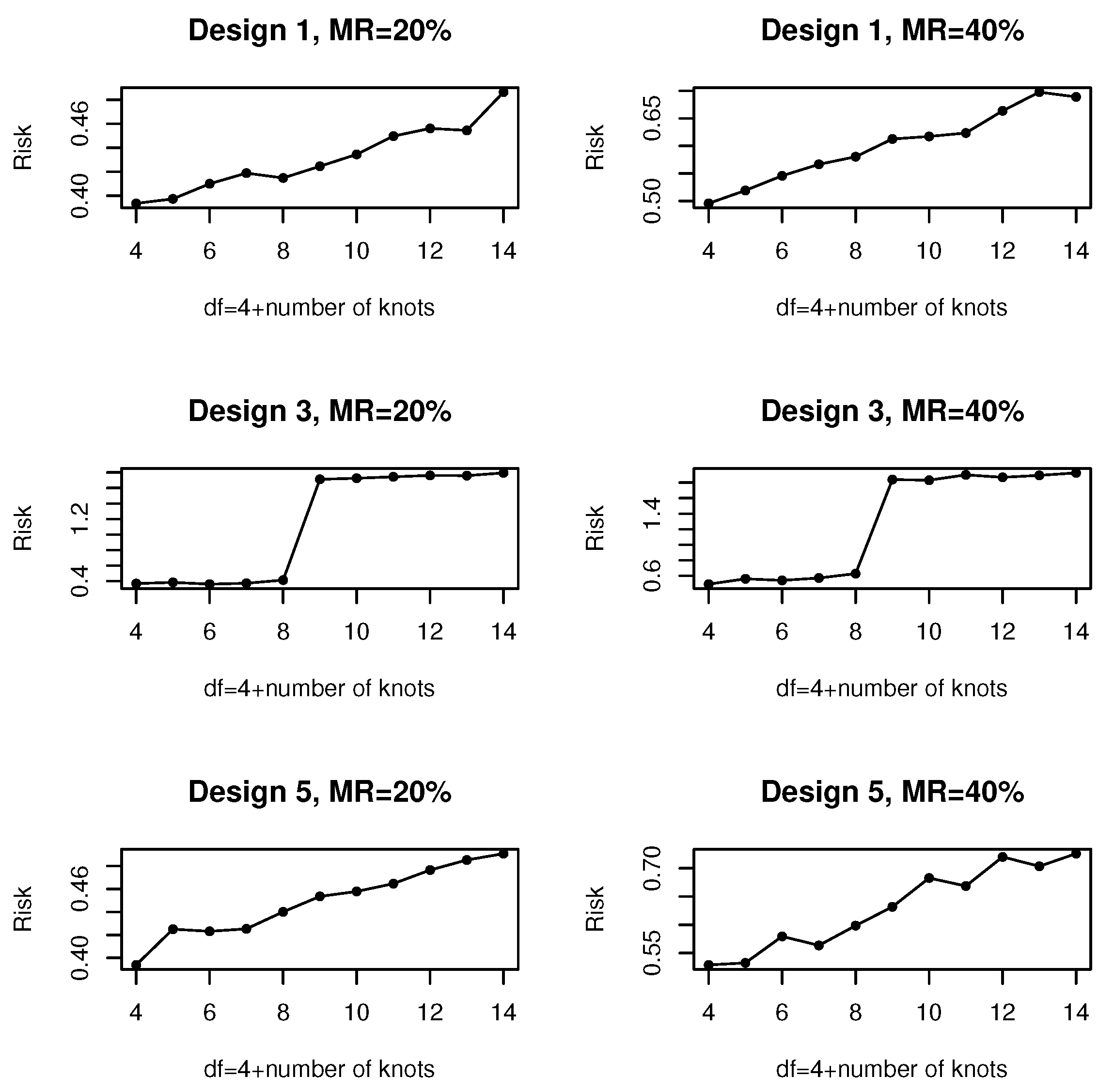
3.2.1. Selection of the Knot Number

We used the cubic B-splines to approximate each nonparametric function, and the spline basis matrix was produced by the function “bs(·, df)” in the“splines” package of the R project, where the degree of freedom df = 4 + number of knots. We assessed the effect of the knot number on the performance of our proposal based on the following risk:

$${\displaystyle L_{\mu }=\frac{1}{1000}\sum _{r=1}^{1000}{\parallel {\widehat{\mu }}_{\widehat{\pi }}{(\widehat{w})}^{(r)}-\mu \parallel }^2,}$$

(17)

where 1000 was the number of simulation trials and ${\widehat{\mu }}_{\widehat{\pi }}{(\widehat{w})}^{(r)}$ was the model averaging estimator of $\mu$ in the rth run.

We set $\zeta =1$ and $n=200$ to show the impact of the number of interior knots on the risk of our proposed procedure in the five designs. Since the simulated results produced were similar for Designs 1 and 2, and for Designs 3 and 4, we only report the results from Designs 1, 3 and 5, which are presented in Figure 2. This figure demonstrates the risk against df for a variety of combinations of designs and missing rates considered. From Figure 2, we note that, for almost all situations considered, generally the risk tended to increase with the number of knots. In other words, the larger number of knots yielded a more serious oversmoothing effect, and, hence, lower estimation accuracy. As suggested by this figure, for our proposed model averaging method, we specified df = 4, which corresponded to the smallest risk. Therefore, in this simulation, we adopted the suggestion of applying df = 4 for all five designs. In other words, the number of knots was set to be 0 in our analysis, which resulted in a basis for ordinary polynomial regression. The number of knots of the B-spline basis function was also set to be 0 in [29], which examined the influence of the knot number on the model averaging method for the varying-coefficient model when all data were available.

3.2.2. Alternative Methods

We conducted some simulation experiments to assess the finite sample performance of our proposed model averaging approach, called the HR$C_p$ approach, in VCPLM with missing data. We compared it with four alternatives, the missing data problems of which were addressed by the IPW method discussed in Section 2. The alternatives included two well-known model selection methods (AIC and BIC) and two widely-used model averaging methods (SAIC and SBIC). Along the lines of [32], we defined the AIC and BIC scores under the varying-coefficient partially linear missing data framework as:

$$AI{C}_m=log({\widehat{\sigma }}_{(m,\widehat{\pi })}^2)+2n^{-1}tr(P_{(m)}),$$

(18)

and

$$BI{C}_m=log({\widehat{\sigma }}_{(m,\widehat{\pi })}^2)+n^{-1}tr(P_{(m)})log(n),$$

(19)

where ${\widehat{\sigma }}_{(m,\widehat{\pi })}^2=n^{-1}{\parallel H_{\widehat{\pi }}-{\widehat{\mu }}_{(m,\widehat{\pi })}\parallel }^2$. These two model selection methods select the model corresponding to the smallest score of the information criterion. The two model averaging methods, SAIC and SBIC, respectively, assign weights:

$$w_{AI{C}_m}=exp(-AI{C}_m/2)/\sum _{m^{\prime }=1}^{M}exp(-AI{C}_{m^{\prime }}/2)$$

(20)

and

$$w_{BI{C}_m}=exp(-BI{C}_m/2)/\sum _{m^{\prime }=1}^{M}exp(-BI{C}_{m^{\prime }}/2)$$

(21)

to the mth candidate model. As suggested by a referee, we also compared our proposal with the Mallows model averaging approach of [29] with a complete-case analysis, which just excluded the individuals with missingness (denoted as CC-MMA). We evaluated the performance of these six methods by computing their risks, and the corresponding results for Designs 1–5 are respectively displayed in Figure 3, Figure 4, Figure 5, Figure 6 and Figure 7. For better comparison, all risks were normalized by the risk of the AIC model selection method.

Besides, following an anonymous referee’s suggestion, we make a comparison of computation time between different model selection and averaging methods. To be more specific, we examined the resulting computation time in seconds by, respectively, employing six methods for five designs when $n=100$, $R^2=0.1$ and MR = $20\%$. The corresponding results are listed in

Table 2. Averaged computation time in seconds over 3 runs, when $n=100$, $R^2=0.1$ and MR $=20\%$.

Method	Design 1	Design 2	Design 3	Design 4	Design 5
AIC	0.213	0.223	0.220	0.223	0.248
BIC	0.220	0.229	0.219	0.218	0.247
SAIC	0.222	0.232	0.224	0.225	0.254
SBIC	0.224	0.229	0.222	0.222	0.249
CC-MMA	0.239	0.233	0.232	0.242	0.261
HR$C_p$	0.251	0.242	0.246	0.254	0.284

.

3.3. Simulation Results

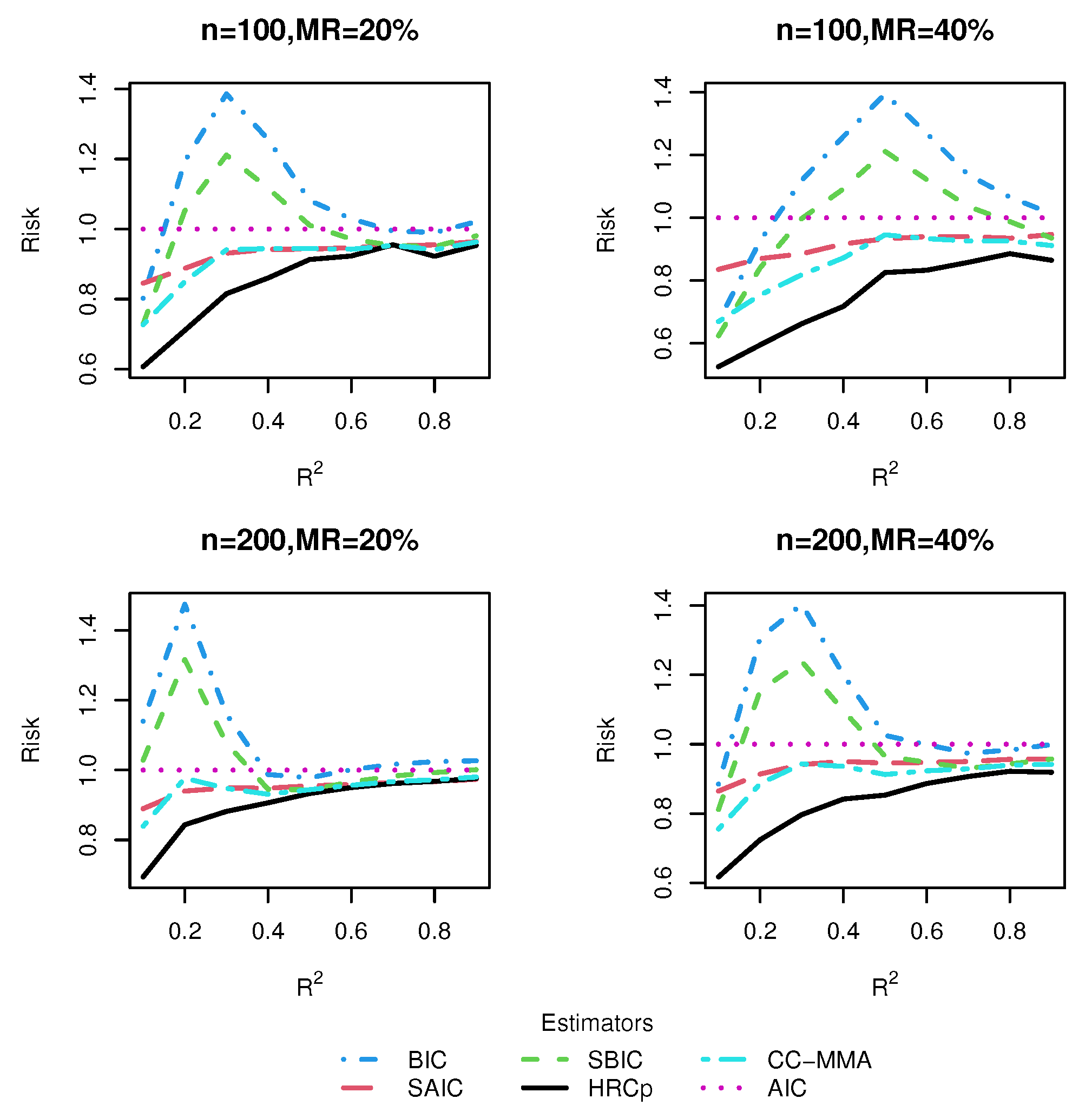
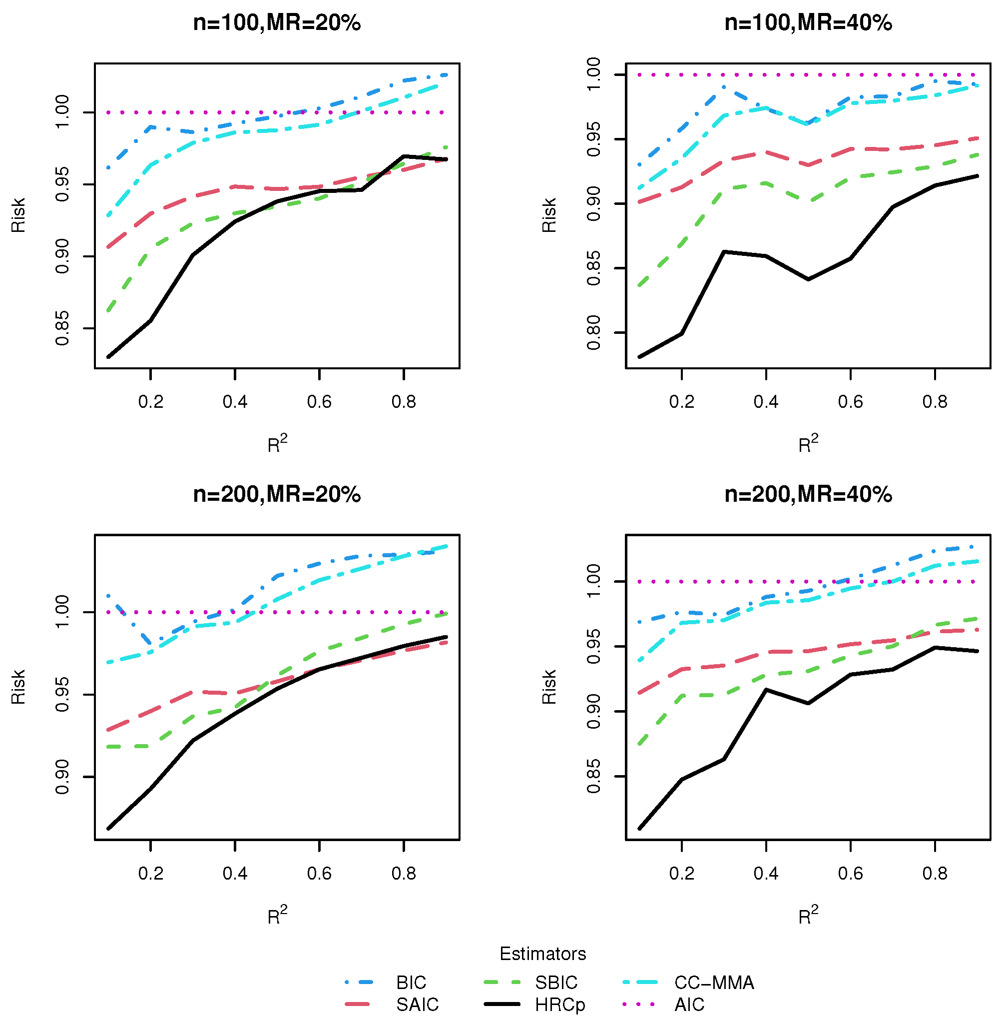
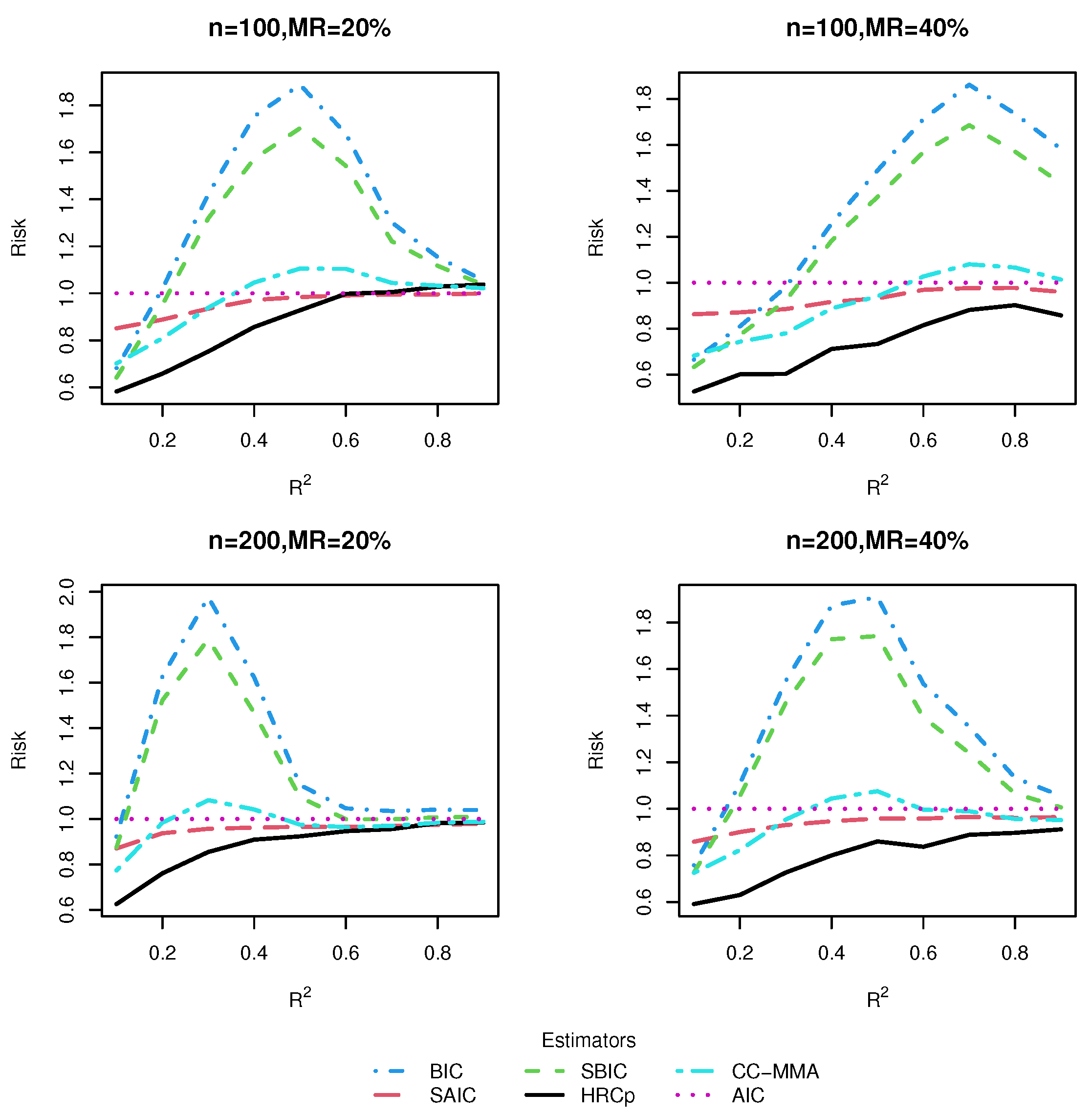
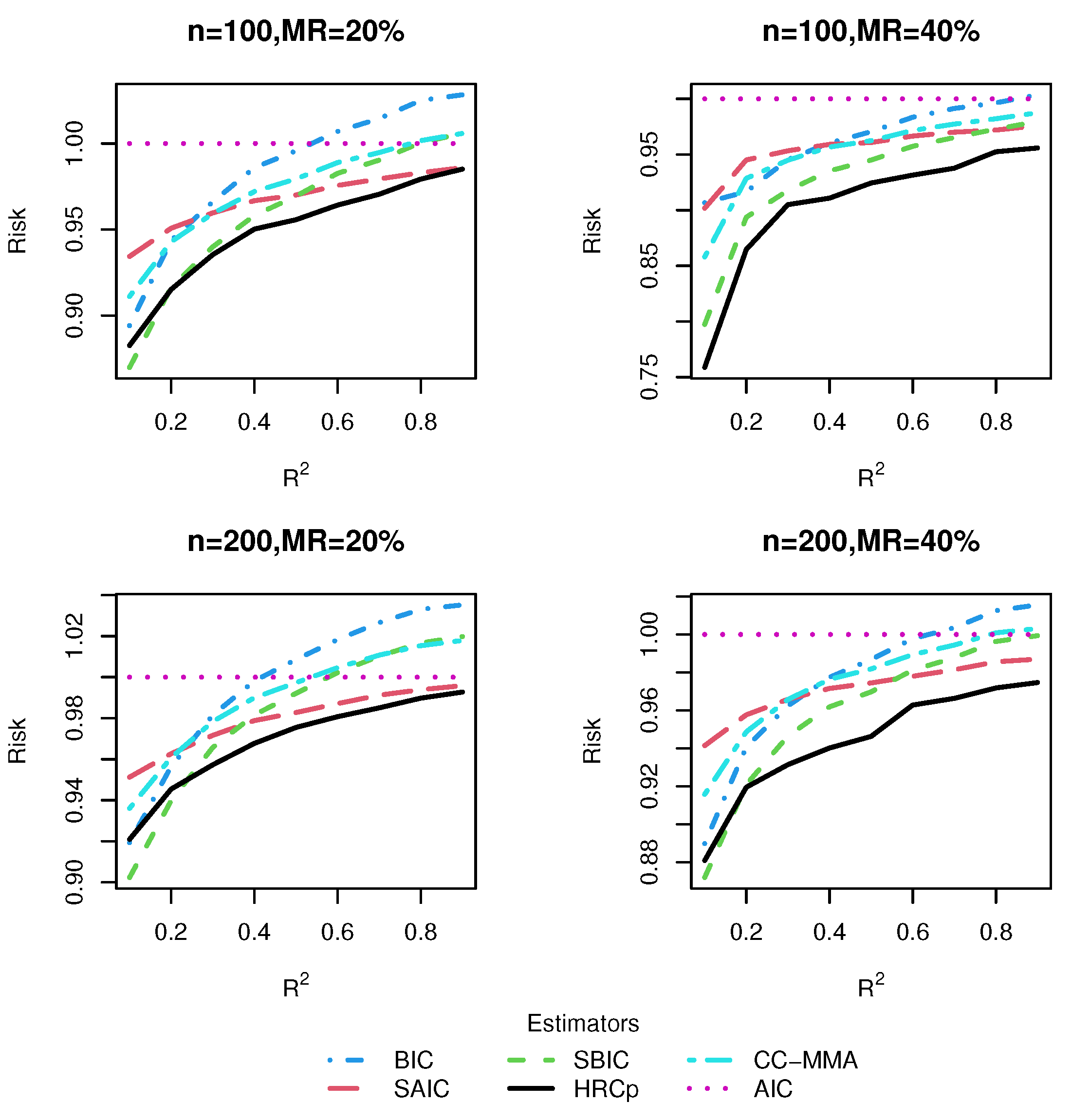
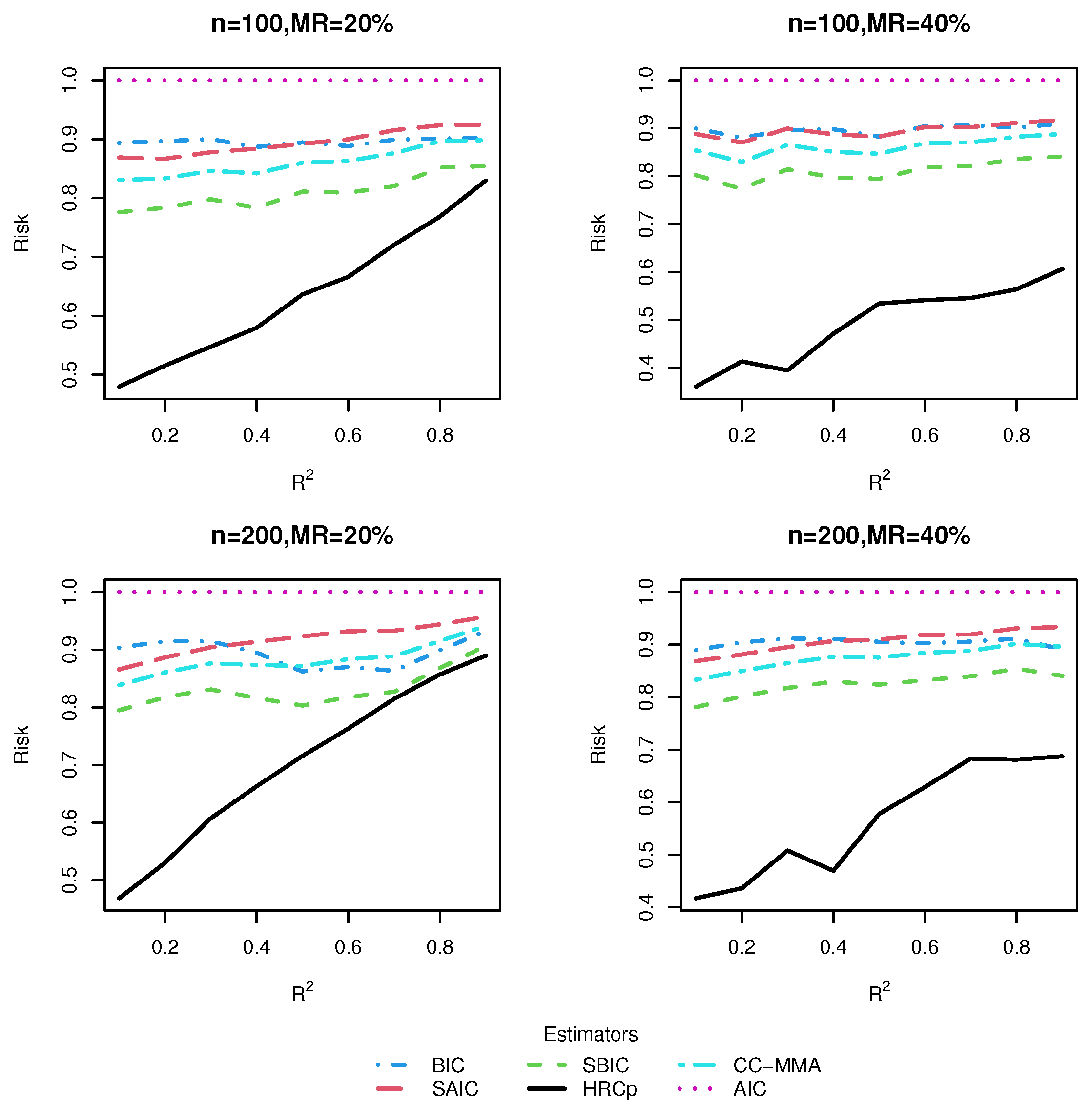
3.3.1. Risk Comparison

From these five figures, we observe that, in general, model averaging approaches worked better than model selection approaches. As shown in most figures, the risk difference in favor of model averaging over model selection was more pronounced when $R^2$ was small or moderate than when $R^2$ was large. This is hardly surprising as it is hard to identify only one best model in the presence of much noise corresponding to a small $R^2$, while the model averaging method shields against selecting a very poor model by compromising across all possible models. On the other hand, when $R^2$ was large, model selection could sometimes be a better strategy than model averaging. A possible reason for this is that the small noise in the data allows the model selection strategy to select the right model with very high frequencies.

As for the comparison of HR$C_p$ method with its rivals, we found that no matter whether the candidate models were nested or not, our proposed model averaging method yielded the smallest risk in almost all combinations of simulation designs, sample sizes and missing rates considered, although when $R^2$ was very high, the information criterion-based model averaging methods could sometimes be marginally preferable to ours. The superiority of our method was more marked in Design 5, which was subject to two kinds of uncertainty simultaneously, uncertainty in covariate inclusion and uncertainty in structure, than in Designs 1–4, which were only associated with uncertainty in the linear part specification. This finding provided evidence that our model averaging method was most effective when both the linear and nonlinear components of the model are uncertain, as in most real-world applications. The good performance of our method in finite samples can be partially explained by noting that the optimality of the HR$C_p$ estimator does not depend on the correct specification of candidate models. As expected, it was observed that information criterion-based model averaging methods invariably produced more accurate estimators than their model selection counterparts. The advantage of our approach became more noticeable as the missing rate increased.

To sum up, within the context of the VCPLM with missing responses, and when the missing data is handled by an IPW method, our proposed HR$C_p$ model averaging method performs better than information criterion-based model selection and averaging methods in terms of risk, especially when the model is characterized by much noise. By and large, our results are parallel to those of [26], which investigated model averaging in the VCPLM with complete data. Additionally, we found evidence of our proposed IPW technique-based model averaging method, HR$C_p$, enjoying significantly smaller risk than a model averaging method with complete-case analysis, CC-MMA.

3.3.2. Computation Time Comparison

According to Table 2, it was hardly surprising that model selection methods always needed less computation time than model averaging methods in all designs. Among all model averaging methods, two data-driven methods (CC-MMA and HR$C_p$) spent slightly more time than the two information criterion-based methods (SAIC and SBIC). As for the comparison between CC-MMA and HR$C_p$, it was expected that our method would perform slightly more slowly than CC-MMA because of the need to approximate the unknown propensity score function. In general, from the perspective of computation time, our method was slightly inferior to other methods, but it greatly dominated its competitors in terms of estimation accuracy. Thus, it is worthwhile to carry out the HR$C_p$ model averaging method to obtain a comparatively accurate estimator, even if a little computation time has to be sacrificed.

4. Real Data Analysis

In this section, we applied our model averaging method to analyze data including information about aged patients from 36 for-profit nursing homes in San Diego, California, provided in [37] and studied by [26,38]. The response variable, y, was the natural logarithm of the days in the nursing home. The five covariates were $x_1$, a binary variable indicating whether the patient was treated at a nursing home; $x_2$, a binary variable indicating whether the patient was male; $x_3$, a binary variable indicating whether the patient was married; $x_4$, a health status variable, with a smaller value indicating better health condition; $u=(\mathrm{age}-64)/(102-64)$, the normalized age of the patients was the effect modifier, with age ranging from 65 to 102.

We considered fitting the data by the VCPLM, but we were not sure which of $x_1$, $x_2$, $x_3$ and $x_4$ to include, and we were uncertain whether to assign a variable in the linear or nonparametric part. Therefore, we considered all possibilities, namely, a variable in the linear part or in the nonparametric part or not in the model. Similar to the simulation study, we required all candidate models to include no fewer than one linear and one nonparametric variable. This resulted in 50 possible models. In our analysis, we ignored 332 censored observations from the original data, and only focused on the remaining 1269 uncensored sample points. Further, we randomly selected $n_0$ observations from the 1269 uncensored observations as the training set and the remaining $n_1=n-n_0$ observations were taken as test set, where $n_0=700,800,900,1000$ and 1100. Since the data points we used could be fully observed, to illustrate the application of our method, we artificially created missing responses in the training data, according to the following missing data mechanism:

$$\mathrm{logit}\{P({\delta }_i=1|X_i,Z_i,u_i)\}=1+0.4u_i+0.4x_{i1}.$$

(22)

Hence, the corresponding mean missing rate was about $20\%$.

We employed observations in the training set to obtain estimators of model parameters in each candidate model, and then performed four model averaging (HR$C_p$, CC-MMA, SAIC and SBIC) and two model selection (AIC and BIC) procedures. We fitted each candidate model by applying the estimation method introduced in Section 2. The cubic B-splines were adopted to approximate each coefficient function. Following the suggestion in the simulation study, we set the number of knots to be 0. We then evaluated the predictive performance of these six approaches by computing their mean squared prediction error (MSPE). As suggested by [4,26], the observations in the test set were utilized to compute the MSPE as follows:

$${\displaystyle \mathrm{MSPE}=\frac{1}{n_1}\sum _{i=n_0+1}^n{(y_i-{\widehat{\mu }}_i)}^2,}$$

(23)

where ${\widehat{\mu }}_i$ is the predicted value for the ith patient based on each approach. We repeated the above process 500 times and calculated the mean, median and standard deviation (SD) of the MSPEs of the six strategies across the replications. For comparison convenience, all MSPEs were normalized by dividing the MSPE of AIC, which was referred to as the relative MSPE (RMSPE). The results are summarized in

Table 3. The mean, median and SD of RMSPE across 500 repetitions.

${\mathit{n}}_{\mathbf{0}}$	Method	BIC	SAIC	SBIC	CC-MMA	HRCp
700	mean	0.991	0.984	0.981	0.989	0.980
	median	0.997	0.989	0.988	0.993	0.985
	SD	0.624	0.660	0.573	0.622	0.619
800	mean	0.993	0.987	0.985	0.990	0.982
	median	0.997	0.990	0.988	0.994	0.985
	SD	0.882	0.909	0.866	0.881	0.884
900	mean	0.994	0.988	0.987	0.991	0.984
	median	0.995	0.989	0.988	0.992	0.986
	SD	0.827	0.861	0.792	0.847	0.836
1000	mean	0.995	0.989	0.988	0.991	0.985
	median	0.997	0.989	0.989	0.992	0.986
	SD	0.890	0.885	0.883	0.888	0.876
1100	mean	0.995	0.990	0.990	0.991	0.986
	median	0.998	0.993	0.991	0.992	0.990
	SD	0.968	0.968	0.957	0.966	0.939

.

The results in Table 3 show that in almost all situations, our proposed HR$C_p$ method had the best predictive efficiency among the six approaches considered. The superiority of our method was particularly obvious in terms of the mean and median, since the smallest mean and median were invariably produced by our method for all training sample sizes. The SBIC always yielded a mean and median that were second to the HR$C_p$ but the best among the remaining five methods. As for the comparison of SD, we found evidence that our method had an edge over other methods when $n_0$ was not less than 1000, while the SBIC frequently yielded the smallest SD when $n_0$ was less than 1000. This implied that our HR$C_p$ method outperformed the SBIC method when the size of the training set was large. We further noted that all numbers in this table were smaller than 1, which implied that the AIC was the worst method among those considered, irrespective of the performance yardstick.

We also provide the Diebold and Mariano test results for the differences in MSPE, which are displayed in

Table 4. Diebold–Mariano test results for the differences in MSPE.

${\mathit{n}}_{\mathbf{0}}$	Method	${\displaystyle \frac{\mathbf{AIC}}{\mathbf{BIC}}}$	${\displaystyle \frac{\mathbf{AIC}}{\mathbf{SAIC}}}$	${\displaystyle \frac{\mathbf{AIC}}{\mathbf{SBIC}}}$	${\displaystyle \frac{\mathbf{AIC}}{\mathbf{CC}-\mathbf{MMA}}}$	${\displaystyle \frac{\mathbf{AIC}}{\mathbf{HRCp}}}$	${\displaystyle \frac{\mathbf{BIC}}{\mathbf{SAIC}}}$	${\displaystyle \frac{\mathbf{BIC}}{\mathbf{SBIC}}}$	${\displaystyle \frac{\mathbf{BIC}}{\mathbf{CC}-\mathbf{MMA}}}$
700	DM	3.622	9.693	7.738	4.147	10.528	6.196	15.908	2.165
	p-value	0.000	0.000	0.000	0.000	0.000	0.000	0.000	0.030
800	DM	5.345	15.916	11.589	9.472	15.832	6.216	18.979	10.863
	p-value	0.000	0.000	0.000	0.000	0.000	0.000	0.000	0.000
900	DM	3.353	10.127	8.009	4.725	11.867	5.502	14.992	5.128
	p-value	0.001	0.000	0.000	0.000	0.000	0.000	0.000	0.000
1000	DM	2.930	9.012	7.165	4.192	12.665	7.697	17.102	3.214
	p-value	0.003	0.000	0.000	0.000	0.000	0.000	0.001	0.001
1100	DM	3.550	12.475	8.565	7.291	13.101	5.299	12.739	4.395
	p-value	0.000	0.000	0.000	0.000	0.000	0.000	0.000	0.000
${\mathit{n}}_{\mathbf{0}}$	Method	${\displaystyle \frac{\mathbf{BIC}}{\mathbf{HRCp}}}$	${\displaystyle \frac{\mathbf{SAIC}}{\mathbf{SBIC}}}$	${\displaystyle \frac{\mathbf{SAIC}}{\mathbf{CC}\mathbf{-}\mathbf{MMA}}}$	${\displaystyle \frac{\mathbf{SAIC}}{\mathbf{HRCp}}}$	${\displaystyle \frac{\mathbf{SBIC}}{\mathbf{CC}\mathbf{-}\mathbf{MMA}}}$	${\displaystyle \frac{\mathbf{SBIC}}{\mathbf{HRCp}}}$	${\displaystyle \frac{\mathbf{CC}\mathbf{-}\mathbf{MMA}}{\mathbf{HRCp}}}$
700	DM	9.173	3.452	−4.682	6.001	−7.245	0.942	11.426
	p-value	0.000	0.001	0.000	0.000	0.000	0.346	0.000
800	DM	12.102	3.276	−4.274	8.501	−6.835	1.827	12.183
	p-value	0.000	0.001	0.000	0.000	0.000	0.068	0.000
900	DM	8.740	2.935	−1.231	7.078	−5.352	1.301	10.278
	p-value	0.000	0.000	0.218	0.000	0.000	0.193	0.000
1000	DM	10.586	1.404	−2.053	8.353	−2.975	3.537	9.486
	p-value	0.000	0.160	0.040	0.000	0.003	0.000	0.000
1100	DM	9.937	1.154	−0.892	7.721	−1.626	4.149	11.254
	p-value	0.006	0.249	0.372	0.000	0.104	0.000	0.000

. A positive/negative test statistic in this table denotes that the estimator in the numerator leads to a bigger/smaller MSPE than the estimator in the denominator. The test statistics and p-values listed in columns 3, 6, 7 and 9 provide evidence that the MSPE differences between our proposed HR$C_p$ estimator and the BIC, SAIC, AIC and CC-MMA estimators were statistically significant for all training set sizes. Considering the HR$C_p$ and SBIC estimators, column 8 demonstrates that the advantage of HR$C_p$ over SBIC was statistically significant in the case with $n_0=1000$ and 1100. However, the same cannot be reported about the differences in performance between the HR$C_p$ and SBIC estimators when $n_0$ was less than 1000, as presented in column 8. This result reinforced the intuition that the HR$C_p$ estimator was more reliable than the SBIC estimator when the training set size was large. The test results shown in columns 3–7 indicate that the MSPE differences between AIC estimator and the remaining five estimators were statistically significant in all situations. The test results given in columns 3, 8, 9 and 10 imply the same about the differences between the BIC and the other five estimators.

5. Conclusions

Considering model averaging estimation in the VCPLM with missing responses, we propose a HR$C_p$ weight choice criterion and its feasible form. Our model averaging process can jointly incorporate two layers of model uncertainty: the first concerns which covariates to include and the second further concerns whether a covariate should be in the linear or nonparametric component. The resultant model averaging estimator is shown to be asymptotically optimal in the sense of achieving the lowest possible squared error loss under certain regularity conditions. The simulation results demonstrated that, in several designs with different types of model uncertainty, our model averaging method always performed much better in comparison with existing methods. The real data analysis also reveals the superiority of the proposed strategy.

There are still many issues deserving future research. Firstly, we only considered model averaging for the VCPLM in the context of missing response data, so it would be worthwhile considering cases where some covariates are also subject to missingness, or missing data arise in a more general framework, such as the generalized VCPLM which permits a discrete response variable. Secondly, in our analysis the missing data mechanism was MAR. The development of a model averaging procedure in a more natural, but more complex, non-ignorable missing data case and the establishment of its asymptotic property is still challenging and warrants future studies. Thirdly, our procedure is applicable only when the dimension parameters $p_m$ and $q_m$ are less than the sample size n. The consideration of an asymptotically optimal model averaging method for high dimensional VCPLM with missing data is meaningful and, thus, merits future research.

References

1. Hansen, B.E. Least squares model averaging. Econometrica 2007, 75, 1175–1189. [Google Scholar] [CrossRef]
2. Wan, A.T.K.; Zhang, X.; Zou, G. Least squares model averaging by Mallows criterion. J. Economet. 2010, 156, 277–283. [Google Scholar] [CrossRef]
3. Liang, H.; Zou, G.; Wan, A.T.K.; Zhang, X. Optimal weight choice for frequentist model average estimators. J. Am. Stat. Assoc. 2011, 106, 1053–1066. [Google Scholar] [CrossRef]
4. Hansen, B.E.; Racine, J.S. Jackknife model averaging. J. Economet. 2012, 167, 38–46. [Google Scholar] [CrossRef]
5. Zhang, X.; Wan, A.T.K.; Zou, G. Model averaging by jackknife criterion in models with dependent data. J. Economet. 2013, 174, 82–94. [Google Scholar] [CrossRef]
6. Lu, X.; Su, L. Jackknife model averaging for quantile regressions. J. Economet. 2015, 188, 40–58. [Google Scholar] [CrossRef]
7. Liu, Q.; Okui, R. Heteroscedasticity-robust Cp model averaging. Economet. J. 2013, 16, 463–472. [Google Scholar] [CrossRef]
8. Zhang, X.; Zou, G.; Carroll, R.J. Model averaging based on Kullback-Leibler distance. Stat. Sinica 2015, 25, 1583–1598. [Google Scholar] [CrossRef] [PubMed]
9. Zhu, R.; Zhang, X.; Wan, A.T.K.; Zou, G. Kernel averaging estimators. J. Bus. Econ. Stat. 2022, 41, 157–169. [Google Scholar] [CrossRef]
10. Zhang, X.; Liu, C.A. Model averaging prediction by K-fold cross-validation. J. Economet. 2022, in press. [Google Scholar]
11. Zhang, X. Model averaging with covariates that are missing completely at random. Econ. Lett. 2013, 121, 360–363. [Google Scholar] [CrossRef]
12. Fang, F.; Lan, W.; Tong, J.; Shao, J. Model averaging for prediction with fragmentary data. J. Bus. Econ. Stat. 2019, 37, 517–527. [Google Scholar] [CrossRef]
13. Wei, Y.; Wang, Q.; Liu, W. Model averaging for linear models with responses missing at random. Ann. I. Stat. Math. 2021, 73, 535–553. [Google Scholar] [CrossRef]
14. Wei, Y.; Wang, Q. Cross-validation-based model averaging in linear models with responses missing at random. Stat. Probabil. Lett. 2021, 171, 108990. [Google Scholar] [CrossRef]
15. Xie, J.; Yan, X.; Tang, N. A model-averaging method for high-dimensional regression with missing responses at random. Stat. Sinica 2021, 31, 1005–1026. [Google Scholar] [CrossRef]
16. Li, Q.; Huang, C.J.; Li, D.; Fu, T.T. Semiparametric smooth coefficient models. J. Bus. Econ. Stat. 2002, 20, 412–422. [Google Scholar] [CrossRef]
17. Zhang, W.; Lee, S.Y.; Song, X. Local polynomial fitting in semivarying coefficient model. J. Multivariate Anal. 2002, 82, 166–188. [Google Scholar] [CrossRef]
18. Ahmad, I.; Leelahanon, S.; Li, Q. Efficient estimation of a semiparametric partially linear varying coefficient model. Ann. Stat. 2005, 33, 258–283. [Google Scholar] [CrossRef]
19. Fan, J.; Huang, T. Profile likelihood inferences on semiparametric varying-coefficient partially linear models. Bernoulli 2005, 11, 1031–1057. [Google Scholar] [CrossRef]
20. Li, R.; Liang, H. Variable selection in semiparametric regression modeling. Ann. Stat. 2008, 36, 261–286. [Google Scholar] [CrossRef]
21. Zhao, P.; Xue, L. Variable selection for semiparametric varying coefficient partially linear models. Stat. Probabil. Lett. 2009, 79, 2148–2157. [Google Scholar] [CrossRef]
22. Zhao, P.; Xue, L. Variable selection for semiparametric varying coefficient partially linear errors-in-variables models. J. Multivariate Anal. 2010, 101, 1872–1883. [Google Scholar] [CrossRef]
23. Zhao, W.; Zhang, R.; Liu, J.; Lv, Y. Robust and efficient variable selection for semiparametric partially linear varying coefficient model based on modal regression. Ann. I. Stat. Math. 2014, 66, 165–191. [Google Scholar] [CrossRef]
24. Wang, H.; Zou, G.; Wan, A.T.K. Model averaging for varying-coefficient partially linear measurement error models. Electron. J. Stat. 2012, 6, 1017–1039. [Google Scholar] [CrossRef]
25. Zeng, J.; Cheng, W.; Hu, G.; Rong, Y. Model averaging procedure for varying-coefficient partially linear models with missing responses. J. Korean Stat. Soc. 2018, 47, 379–394. [Google Scholar] [CrossRef]
26. Zhu, R.; Wan, A.T.K.; Zhang, X.; Zou, G. A Mallows-type model averaging estimator for the varying-coefficient partially linear model. J. Am. Stat. Assoc. 2019, 114, 882–892. [Google Scholar] [CrossRef]
27. Hjort, N.L.; Claeskens, G. Frequentist model average estimators. J. Am. Stat. Assoc. 2003, 98, 879–899. [Google Scholar] [CrossRef]
28. Hu, G.; Cheng, W.; Zeng, J. Model averaging by jackknife criterion for varying-coefficient partially linear models. Commun. Stat.-Theor. M. 2020, 49, 2671–2689. [Google Scholar] [CrossRef]
29. Xia, X. Model averaging prediction for nonparametric varying-coefficient models with B-spline smoothing. Stat. Pap. 2021, 62, 2885–2905. [Google Scholar] [CrossRef]
30. Zhang, X.; Wang, W. Optimal model averaging estimation for partially linear models. Stat. Sinica 2019, 29, 693–718. [Google Scholar] [CrossRef]
31. White, J. Maximum likelihood estimation of misspecified models. Econometrica 1982, 50, 1–25. [Google Scholar] [CrossRef]
32. Liang, Z.; Chen, X.; Zhou, Y. Mallows model averaging estimation for linear regression model with right censored data. Acta Math. Appl. Sin. E. 2022, 38, 5–23. [Google Scholar] [CrossRef]
33. Zhang, X.; Liang, H. Focused information criterion and model averaging for generalized additive partial linear models. Ann. Stat. 2011, 39, 174–200. [Google Scholar] [CrossRef]
34. Li, K.C. Asymptotic optimality for Cp, CL, cross-validation and generalized cross-validation: Discrete index set. Ann. Stat. 1987, 15, 958–975. [Google Scholar] [CrossRef]
35. Zhang, X.; Yu, D.; Zou, G.; Liang, H. Optimal model averaging estimation for generalized linear models and generalized linear mixed-effects models. J. Am. Stat. Assoc. 2016, 111, 1775–1790. [Google Scholar] [CrossRef]
36. Ando, T.; Li, K.C. A weighted-relaxed model averaging approach for high-dimensional generalized linear models. Ann. Stat. 2017, 45, 2654–2679. [Google Scholar] [CrossRef]
37. Morris, C.N.; Norton, E.C.; Zhou, X.H. Parametric duration analysis of nursing home usage. In Case Studies in Biometry; Lang, N., Ryan, L., Billard, L., Brillinger, D., Conquest, L., Greenhouse, J., Eds.; Wiley: New York, NY, USA, 1994. [Google Scholar]
38. Fan, J.; Lin, H.; Zhou, Y. Local partial-likelihood estimation for lifetime data. Ann. Stat. 2006, 34, 290–325. [Google Scholar] [CrossRef]
39. Whittle, P. Bounds for the moments of linear and quadratic forms in independent variables. Theor. Probab. Appl. 1960, 5, 331–335. [Google Scholar] [CrossRef]
Figure 1. The flow chart of our research.
Mathematics 11 01883 g001
Figure 2. The curves of the risk with the number of knots over 1000 replications.
Mathematics 11 01883 g002
Figure 3. Risk comparisons for Design 1.
Mathematics 11 01883 g003
Figure 4. Risk comparisons for Design 2.
Mathematics 11 01883 g004
Figure 5. Risk comparisons for Design 3.
Mathematics 11 01883 g005
Figure 6. Risk comparisons for Design 4.
Mathematics 11 01883 g006
Figure 7. Risk comparisons for Design 5.
Mathematics 11 01883 g007