1. Introduction
Deep learning and computer vision (CV) algorithms have recently shown their capabilities in addressing various challenging industrial and scientific problems [
1]. Successful application of machine learning and computer vision algorithms for solving complex tasks is impossible without relying on comprehensive and high-quality training and testing data [
2,
3]. CV algorithms for solving classification, object detection, and semantic and instance segmentation require a huge variety of input data to ensure robust work of the trained models [
4,
5,
6]. There are two major ways to enlarge a training dataset. The first one is obvious and implies physical collection of the dataset samples in various conditions to ensure high diversity of the training data. There is a set of huge datasets that have been collected for solving computer vision problems. These datasets are commonly used as the benchmark [
7,
8,
9,
10]. One of the specifics of these datasets is that they are general-domain sets. Unfortunately, general-domain-labeled data can be almost useless for solving specific industrial problems. One of the feasible applications of such well-known datasets is that they can serve as a good basis for pre-training of neural networks (transfer learning) [
11,
12]. Using these pre-trained neural networks, it is possible to fine-tune them and adapt them to address specific problems. However, in some cases, even for fine-tuning, a comprehensive dataset is in high demand. Some events are rare, and it is possible to collect only a few data samples [
13,
14,
15]. Thus, a second approach for enhancing the characteristics of the dataset can help. This approach is based on artificial manipulations with the initial dataset [
16,
17]. One of the well-developed techniques is data augmentation, where original images are transformed according to special rules [
18]. Usually, the goal of image augmentation is to make the training dataset more diverse. However, augmentation can be used to deliberately shift the data distribution. If the distribution of the original training dataset differs from the distribution of the test set, it is important to equalize them as much as possible.
The agricultural domain is part of the industrial and research areas for which the development of artificial methods for improvement of training datasets is vital [
19,
20,
21]. This demand appears due to the high complexity and variability of the investigated system (plant) that has to be characterized by computer vision algorithms [
22]. The difficulty of the agricultural domain makes it a good candidate for testing augmentation algorithms.
There are many different plant species, and plants grow slowly. Thus, collecting and labeling huge datasets for each specific plant growing in each specific stage is a complex task [
23]. Overall, it is difficult to collect datasets [
24], especially for plants, and it is expensive to annotate them [
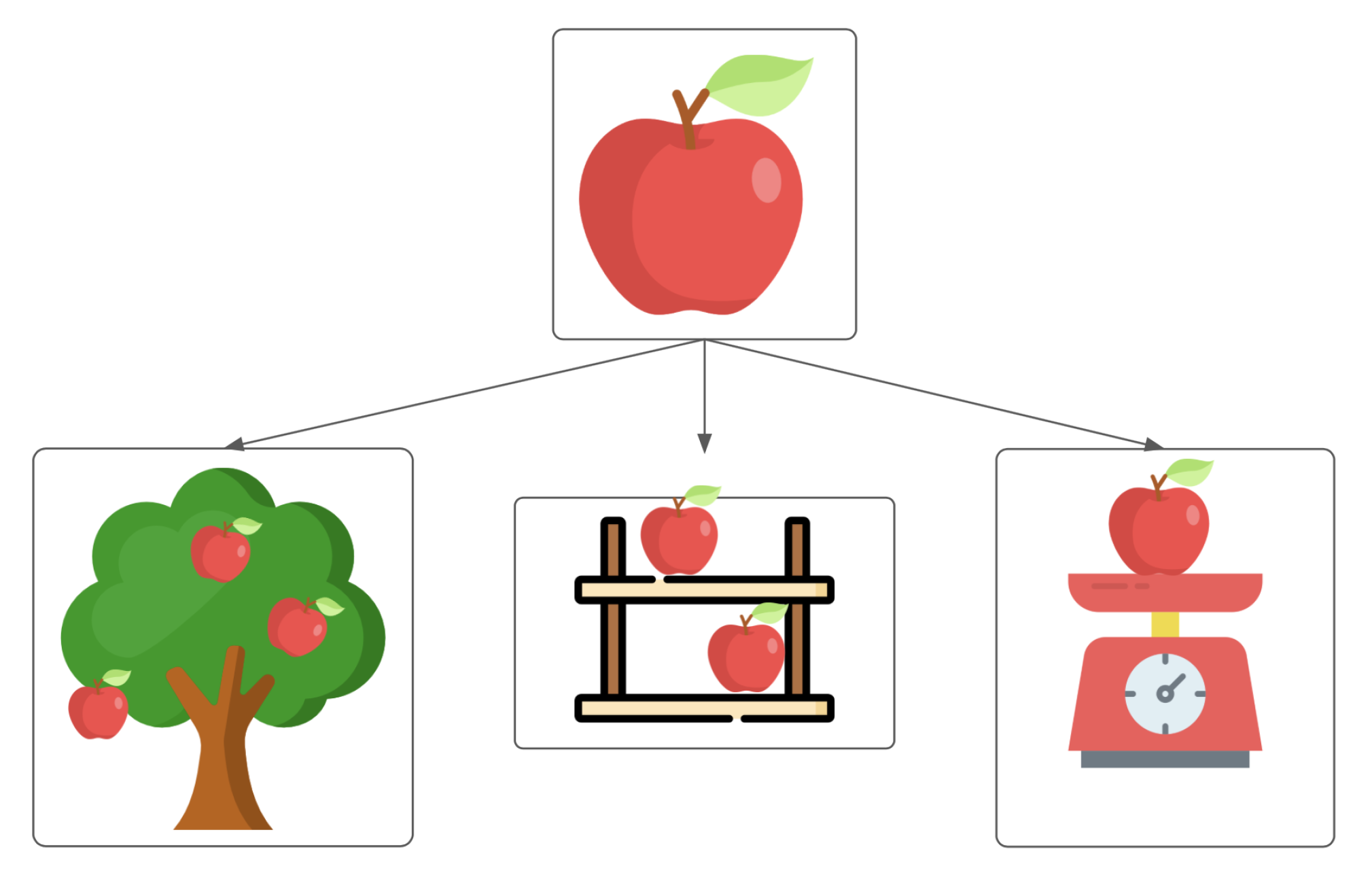
25]. Therefore, we propose a method to multiply the number of training samples. It does not require many computational resources, and it can be performed on the fly. The idea behind the algorithm is to cut instances from the original images and add them onto the new backgrounds (
Figure 1).
The contribution of this study is the following:
we describe an efficient algorithm for instance-level image augmentation and measure its performance;
we prove that the context is vital for instance-level augmentation;
we propose several efficient ways to find representative background images if the test environment context is known;
we show that it is possible to estimate which dataset variant will provide better accuracy before model training, calculating the FID between the test dataset and the training dataset variants;
we share the dataset and generate background images and source code for augmentation.
The novelty of this study is as follows:
extensive experiments with instance-level augmentation for different computer vision tasks;
experiments with different model types;
application of FID to choose the augmentation approach.
1.1. Image Augmentation
Computer vision models require many training data. Therefore, it becomes challenging to obtain a good model with limited datasets. Namely, a small-capacity model might not capture complex patterns, while a big capacity model tends to overfit if small datasets are used [
26]. Slight changes in test data connected with surrounding and environmental conditions might also lead to a decrease in model performance [
27].
To overcome this issue, we use various image augmentation techniques. Data augmentation aims to add diversity to the training set and to complicate the task for a model [
28]. Among these plant image augmentation approaches, we can distinguish: basic computer vision augmentations, learned augmentation, graphical modeling, augmentation policy learning, collaging, and compositions of the ones above.
Basic computer vision augmentations are the default methods preventing overfitting in most computer vision tasks. They include image cropping, scaling, flipping, rotating, and adding noise [
29]. There are also advanced augmentation methods, connected with distortion techniques and coordinate system changes [
30]. Since these operations are quite generic, most popular ML frameworks support them. However, although helpful, these methods demonstrate limited use, as they bring insufficient diversity to the training data for few-shot learning cases.
Learned augmentation stands for generating training samples with an ML model. For this purpose, conditional generative adversarial networks (cGANs) and variational autoencoders (VAEs) are frequently used. In the agricultural domain, there are examples of applying GANs to
Arabidopsis plant images for the leaf counting task [
31,
32]. The main drawback of this approach is that generating an image with a neural network is quite resource-intensive. Another disadvantage is the overall pipeline complexity: the errors of a model that generates training samples are accumulated with the errors of a model that solves the target task.
Learned augmentation policy is a series of techniques used to find combinations of basic augmentations that maximize model generalization. This implies hard binding of the learned policy to the ML model, the dataset, and the task. Although it is shown to provide systematic generalization improvement on object detection [
33] and classification [
34], its universal character as well as the ability to be performed along with multi-task learning are not supported with solid evidence.
Collaging presupposes cropping an object from an input image with the help of a manually annotated mask and pasting it to a new background with basic augmentations of each object [
19]. In [
35], a scene generation technique using object mask was successfully implemented for an instance detection task. It boosted model performance significantly compared with the use of only original images. The study on image augmentation for instance segmentation using a copy–paste technique with object mask was extended in [
36]. The importance of scene context for image augmentation is explored in [
37,
38].
1.2. Image Synthesis
Graphical modeling is another popular method in plant phenomics. It involves creating a 3D model of the object of interest and rendering it. The advantage of this process is that it permits the generation of large datasets [
39] with precise annotations, as the labels of each pixel are known. However, this technique is highly resource-intensive; moreover, the results obtained using the existing solutions [
40,
41] seem artificial. More realistic synthesis is very time-consuming. This approach is suitable when there are not many variations of the modeled object. If there are many different object types, it can be easier to collect and annotate new images.
1.3. Neural Image Generation and Image Retrieval
To gain new training images for CV tasks, one can implement GAN-based or diffusion-based models. Currently, they allow for the creation of rather realistic images and meet the demands of different domains, such as agricultural [
42], manufacturing processes [
43], remote sensing [
44], or medical [
45]. Such models can be considered as a part of an image recognition pipeline. Moreover, recent results in Natural Language Processing (NLP) offer opportunities to extend image generation applications via textual description. For instance, an image can be generated based on a proposed prompt, namely, a phrase or a word. Such synthetic images help to extend the initial dataset. The same target image can be described by a broad variety of words and phrases that lead to diverse visual results. Another way to obtain additional training images is a data retrieval approach. It supposes to search for existing images from the Internet or some database according to a user’s prompt. For instance, the CLIP model can be used to compute embedding of a text and to find images that match it better based on distance in a special embedding space [
46].
2. Materials and Methods
The notation that we use in this section for describing the augmentation framework parameters is listed in
Table 1.
2.1. Method Development and Description
In this paper, we introduce a method of image augmentation for a semantic segmentation task. When instance-level annotation areas are available, one can apply our method for other tasks such as classification, object detection, object counting, and semantic segmentation. Our method takes image–mask pairs and transforms them to obtain various scenes. Having a set of image–mask pairs, we can place many of them on a new background. Transformation of input data and background, accompanied by adding noise, gives the possibility for us to synthesize an infinite number of compound scenes.
This section first describes the overall augmentation pipeline and then describes the tested approaches for background image generation.
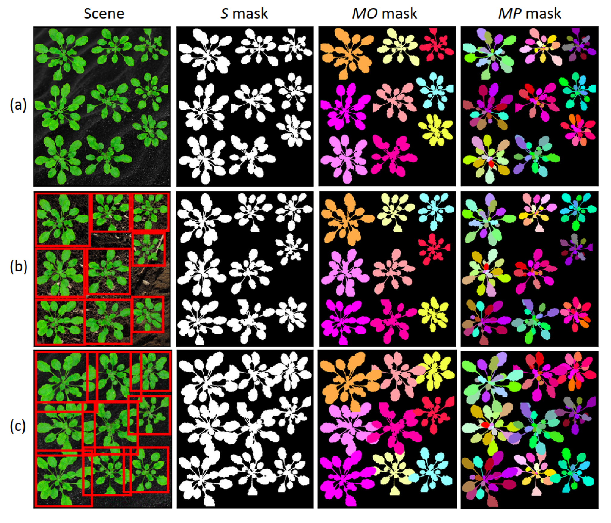
We distinguish between several types of image masks:
Single (S)—single-channel mask that shows the object presence.
Multi-object (MO)—multi-channel mask with a special color for each object (for each plant).
Multi-part (MP)—multi-channel mask with a special color for each object part (for each plant leaf).
Semantic (Sema)—multi-channel mask with a special color for each type of object (leaf, root, flower).
Class (C)—multi-channel mask with a special color for each class (plant variety).
A single-input mask type allows us to produce more than one output mask type. Hence, multiple tasks can be solved using any dataset, even the one that was not originally designed for these tasks (see
Table 2 for the possible mask transitions).
For example, an image with a multipart mask as input enables us to produce: the
S mask, which is a Boolean representation of any other mask, the
MO mask with unique colors for every object, the
MP mask with a unique color for each part across all the present objects, and the
C mask that distinguishes the classes (
Figure 2). Additionally, for every generated sample, we provide bounding boxes for all objects and the number of objects of each class.
Note that we assume that each input image–mask pair includes a single object. Therefore, we can produce the MO mask based on any other mask. To create the C mask, information about input objects must be provided.
2.2. System Architecture
The library with the code will be shared as an open source code with the community. The core of the presented system is the Augmentor. This class implements all the image and mask transformations. Such transformations as flipping or rotating are mutual for both the image and the mask. We add noise for images only.
From the main Augmentor class, we inherit SingleAugmentor, MultiPartAugmentor and SemanticAugmentor classes, helping to apply different input mask types and to treat them separately. To be more precise, SingleAugmentor is exploited for S input mask type, MultiPartAugmentor is for MP mask type, and SemanticAugmentor is for Sema mask type.
The described above classes are used in the DataGen class, which chooses images for each scene and balances classes if needed. Two principal ways of new scene generation are offline and online. We implement them in SavingDataGen and StreamingDataGen accordingly. Both of the classes take the path to images with corresponding masks as input. The offline data generator produces a new folder with created scenes while the online generator can be used to load data directly to a neural network.
Offline generation is more time-consuming because of additional disk access operations; at the same time, it is performed in advance and thus does not affect model training time. It also makes it easier to manually look through the obtained samples to tune the transformation parameters.
Meanwhile, the online data generator streams its results immediately to the model without saving images on the disk. Furthermore, this type of generator allows us to change parameters on the fly: for instance, the model is trained on easy samples, and then, the complexity may be manipulated based on the loss function.
2.3. Implementation Details
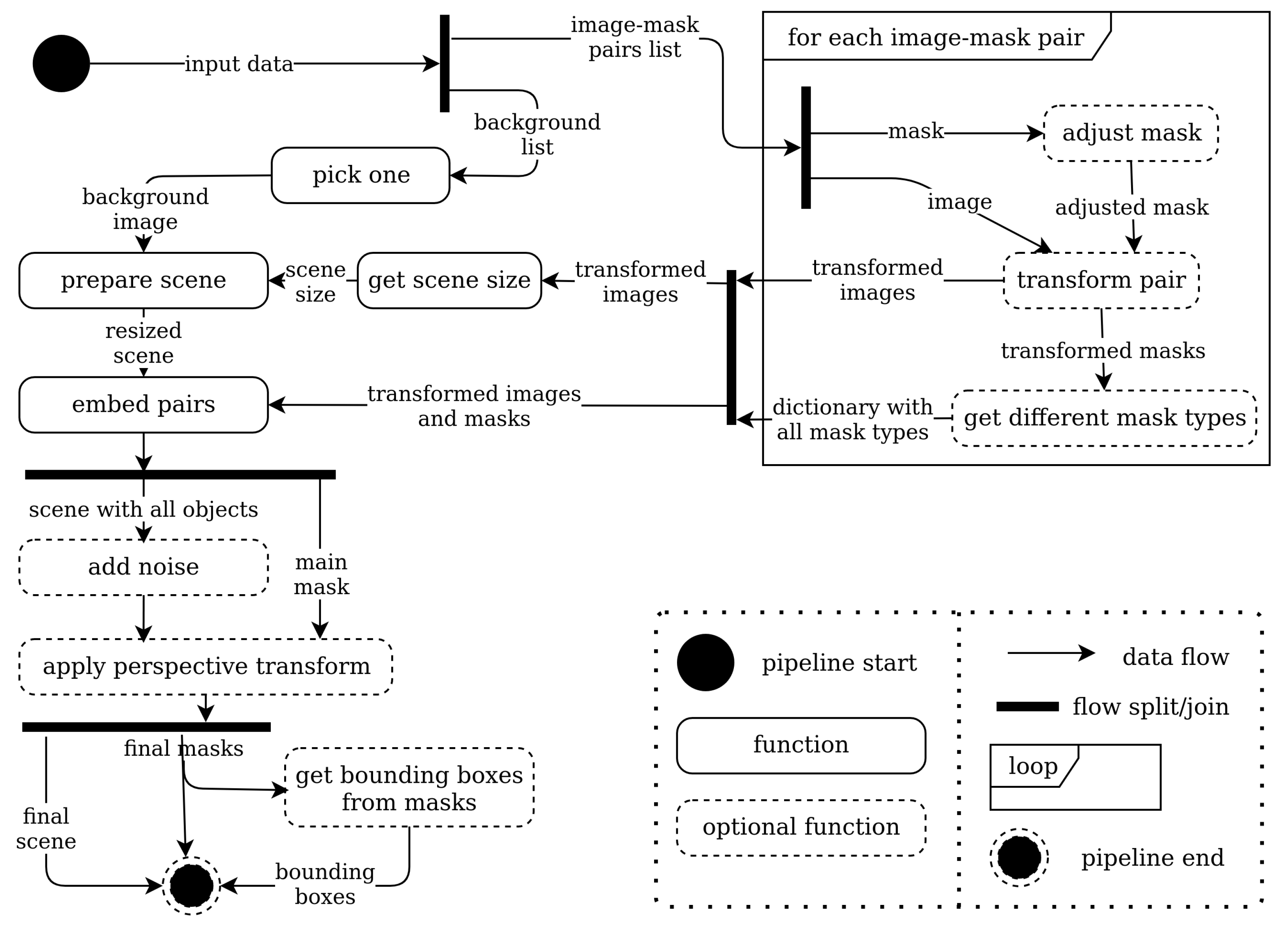
The present section discusses the main transformation pipeline (
Figure 3).
The first step is to select the required number of image–mask pairs from a dataset. By default, we pick objects with repetitions that enable us to create scenes with a larger number of objects than present in the input data.
After that, we prepare images and masks before combining them into a single scene. The procedure is as follows:
adjust the masks to exclude large margins;
perform the same random transformations to both the image and mask;
obtain all required mask types and auxiliary data.
Once all the transformations are performed and we know the sizes of all objects, the size of the output scene is calculated. Note that input objects can have different sizes and orientations; therefore, we cannot simply place objects by grid because it will lead to inefficient space usage. It is also not a good idea to place objects randomly in most cases because it will lead to uncontrollable overlapping of objects.
Within the framework of our approach, the objects are packed using the Maximal Rectangles Best Long Side Fit (MAXRECTS-BLSF) algorithm. It is a greedy algorithm that is aimed at packing rectangles of different sizes into a bin using the smallest possible area. The maximum theoretical packaging space overhead of the MAXRECTS-BLSF algorithm is . The BLSF modification of the algorithm tries to avoid a significant difference between side lengths. However, similar ot other rectangular packing algorithms, this one also tends to abuse the height dimension of the output scene, yielding a column-oriented result.
In order to control both overlapping of the objects and the orientation of output scenes, we introduce two modifications to the MAXRECTS-BLSF algorithm.
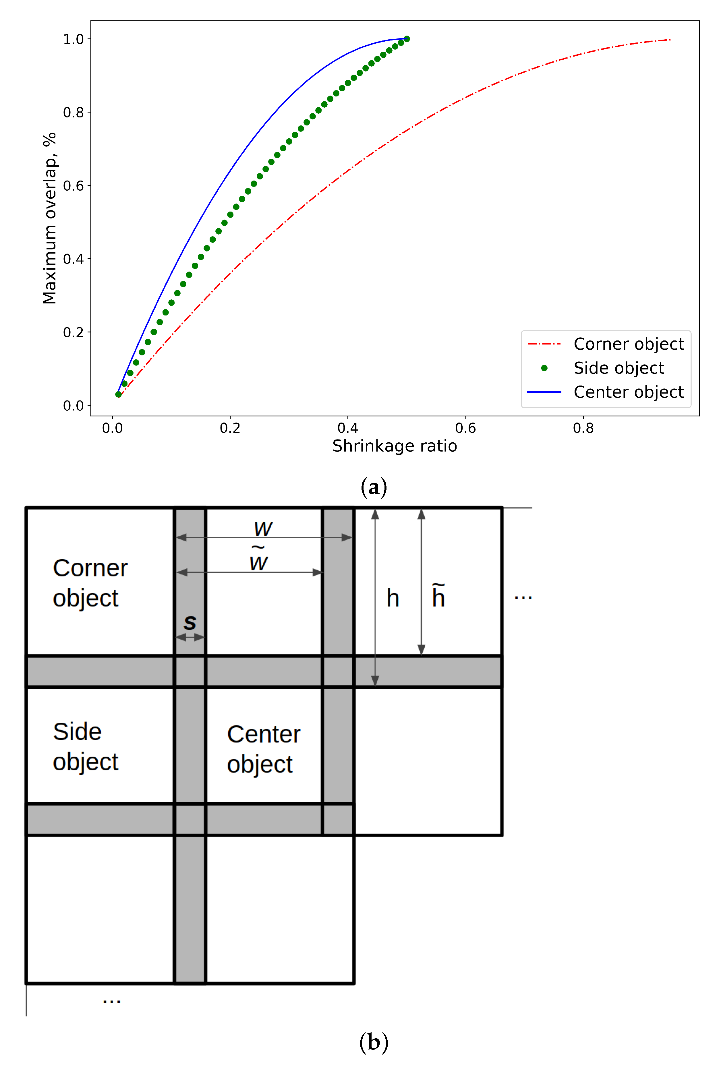
Control of the overlapping is achieved via substituting the objects’ real sizes with the shrinked ones when passing them through the packing algorithm. The height and width are modified according to Equation (
1):
where
s ranges from 0 to 1 inclusively.
The bigger the shrinkage ratio, the smaller the substituted images. It is applied to both height and width and to all of the input objects. The real overlapping area in practice will vary depending on each objects’ shape and position. To perceive the overlap percentage, see
Figure 4. Here, we consider the case where all input objects are squares without any holes. In other words, it is the maximum possible overlap percentage for the defined shrinkage ratio. We show this value for an object in the corner of a scene, an object on the side, and an object in the middle, separately.
We recommend choosing s between 0 and ; however, taking into consideration sparse input masks, it can be slightly higher.
To control the orientation of the output scene, we set a hard limit of the scene height for the packing algorithm. Assuming that input objects will have different sizes in practice, we cannot obtain optimal packing with the fixed output image size or width-to-height ratio. To calculate the hard height limit, we use Equation (
2).
The fraction in Equation (
2) estimates the required value of height to make a square scene. We choose a maximum between it and the biggest objects’ height to ensure that it is enough space for any input object. The orientation coefficient
can be treated as the target width-to-height ratio. It will not produce the scenes with the fixed ratio, but with many samples, the average value will approach the target one.
will try to obtain square scenes.
will generate landscape scenes. In our experiments, we set
to 1.2 to obtain close to square images with landscape preference. The average resulting width-to-height ratio over ten thousand samples was 1.1955.
To adjust the background image size to the obtained scene size, we resize the background if it is smaller than the scene or randomly crop it if it is bigger.
We generate the required number of colors, excluding black and white, and find their Cartesian product according to Algorithm 1 for coloring the
MO and
MP masks.
| Algorithm 1: Color generation. |
Input: Number of objects n; Output: The set of colors C; for do end return |
To preserve the correspondence between the input objects and their representation on the final scene, we color the objects in order of their occurrence.
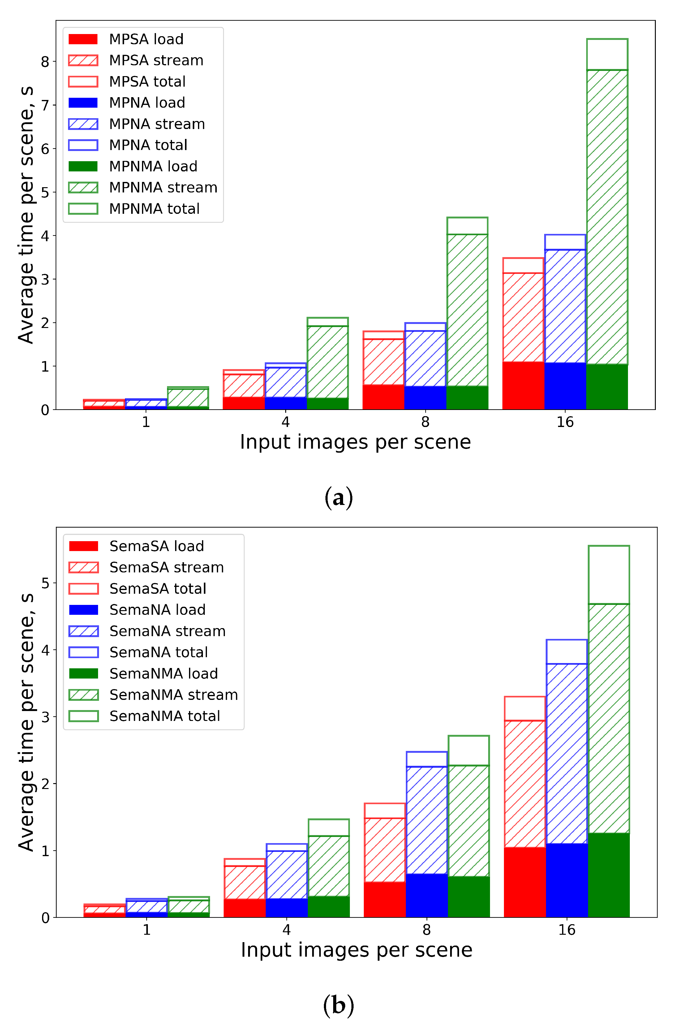
2.4. Time Performance
In this section, we measure the average time that is required to generate scenes of various complexity. For this experiment, we use Intel(R) Core(TM) i7-7700HQ CPU 2.80 GHz without multiprocessing. The average height of objects in the dataset is 385 pixels; the average width is 390 pixels. The results are averaged on a thousand scenes for each parameter combination and are reflected in
Figure 5a for
MultiPartAugmentor and
Figure 5b for
SemanticAugmentor.
SA (the red bar on the left) stands for
Simple Augmentor with one type of output mask;
NA (the blue bar in center) means adding noise and smoothing to scenes;
NMA (the green bar on the right) means adding noise, smoothing, calculating bounding boxes, and generating all possible types of output masks. To recall possible mask types for each augmentor, refer to
Table 2. The filled area in the bottom shows the time for loading input images and masks from disks. The shaded area in the middle shows the time for actual transformation. The empty area in the top shows the time for saving all the results to the disk. If every bar is accumulated with all the bars below it, the top of the shaded bar will show the time for
StreamingDataGen, and the top of the empty area will show the time for
SavingDataGen.
From the bar plots, you can see linear dependence between the number of input objects and the time for generating a scene.
2.5. System Parameters
Two main classes of the system where we can choose parameters are Augmentor and DataGen, or classes inherited.
The
Augmentor parameters that define the transformations are shown in
Table 3.
The rest of the Augmentor parameters define output mask types, bounding box presence, and mask preprocessing steps.
The data generator parameters define the rules to pick samples for scenes: the number of samples per scene, picking samples for a single scene from the same class or randomly, class balancing rule, the input file structure, the output file structure.
2.6. Background Image Choosing
Making many augmented copies of objects is a very powerful tool used to increase dataset variability. However, many previous works underestimate the role of image context. The role of the context in an image plays a role in its background. In this paper, we show that the proper choice of a background is vital. For this, we experiment with methods that produce images that are similar to the test set backgrounds.
In the test set, we have five types of background. It includes: grass, floor tiles, wooden table, color blanket, and shop shelves. Therefore, we want to obtain suitable images that represent every surrounding type. The corresponding text prompts are:
grass: grass, green grass, grass on the Earth, photo of grass, grass grown on the Earth;
floor tiles: tile, ceramic tile, beige tile, grey tile, metal, photo of metal sheet, metal sheet, tile on the floor, close photo of tile, close photo of grey tile;
wooden table: wood, wooden, wooden table, dark wooden table, light wooden table, close photo of wooden table, close photo of table in the room;
color blanket: veil, cover, blanket, color blanket, dark blanket, blanket spread, bed linen, close photo of veil (cover, blanket), blanket on the bed, towel, green towel, close photo of towel on the table;
shop shelves: shelves, shop shelves, close photo of shop shelves, white shop shelves, shop shelves close, table in shop, empty shelves in the shop, table with scales in front of shop shelves, scales in the shop.
We also split backgrounds into easy: wooden table, floor tiles; and complex: grass, color blanket, shop shelves. This split is manual and serves to demonstrate the difference in performance between more and less realistic images. More precisely, complex backgrounds are ones where visual augmentation looks unrealistic. Various background properties are significant not only in the agriculture domain, they represent different environmental conditions in the remote sensing domain and can be considered to boost model performance through geographical regions [
47]. Background complexity in CV tasks for self-driving cars depends on urban area complexity and lighting conditions and has to be taken into account to develop robust algorithms [
48]. To capture observed scenes for aerial vehicle navigation, surrounding properties are also crucial [
49].
We use the described above text prompts with ruDALL-E [
50] and stable diffusion [
51] models to generate similar images, and with the CLIP [
52] model to retrieve similar images from the LAION-400M [
53] dataset. There are 100 collected backgrounds for each prompt.
For the comparison, we also add the worst-case and the best-case backgrounds. As the worst case, we propose to use random pattern images. The best case is to have real images from the same place, where a CV model will be inferenced.
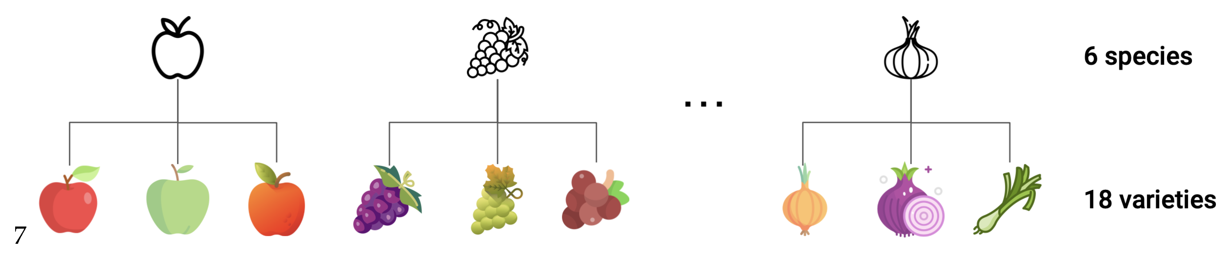
Dataset
To verify the proposed approach, we conduct experiments using a set of images of various fruits and vegetables. We collect a unique dataset that comprises the following species: apple, cabbage, grape, tomato, pepper sweet, and onion. The dataset has hierarchical structure where each species includes three varieties, as is depicted in
Figure 6. All species and varieties are presented in
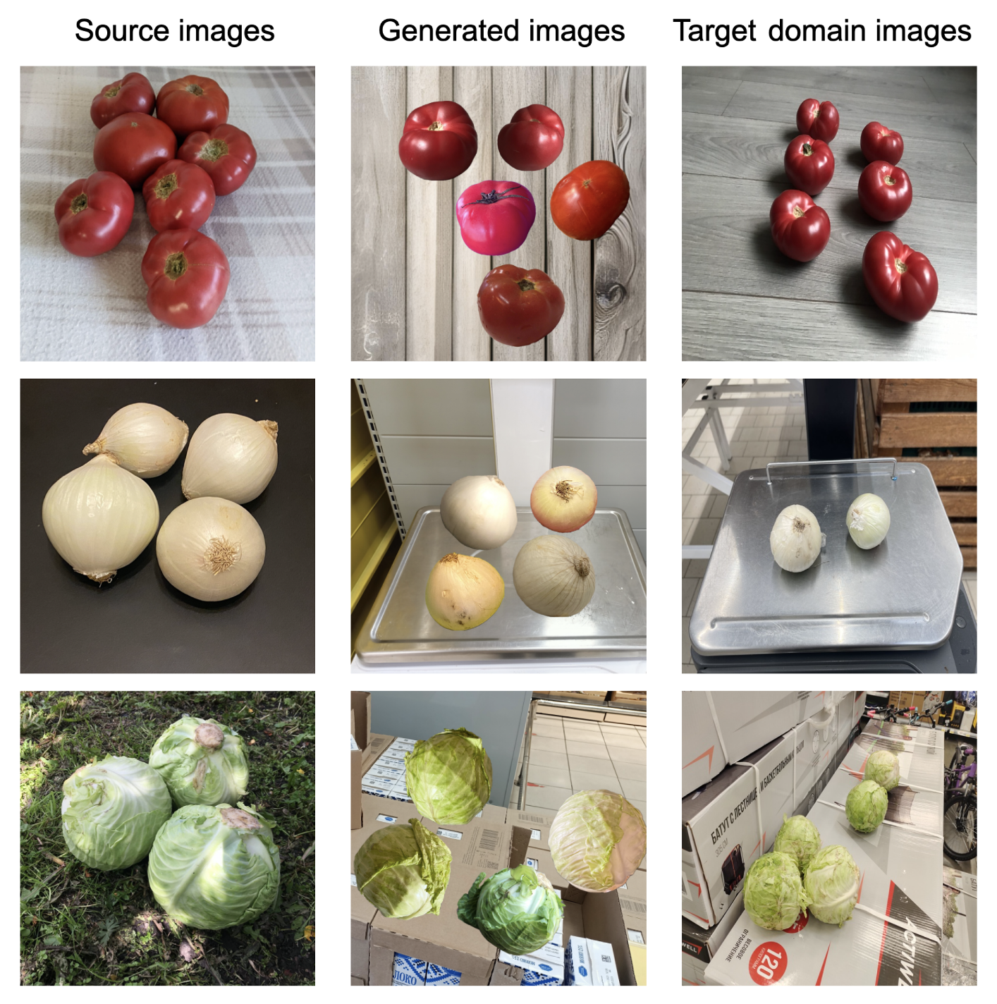
Table 4. Overall, each individual fruit or vegetable variety is represented by 150 images gained in different environmental and lighting conditions. We create a manual instance segmentation annotation for the images. Each image contains several fruits or vegetables of a single variety. Therefore, instance segmentation markup can be easily automatically converted into image classification labels. We can also obtain bounding boxes for object detection based on instance segmentation masks. Hence, we create annotations for three CV tasks, namely, semantic segmentation, image classification, and object detection. For each task, the dataset is split into training and testing in an 80/20 ratio.
Figure 7 depicts generated images using the original dataset with instance segmentation masks.
2.7. Experiments
The experiment setup is as follows. We have to test the stability of our approach under various conditions. For this, we experiment with three CV tasks:
image classification;
semantic segmentation;
object detection.
For each task, we compare:
For the classification task, we also compare different type of models:
convolutional model (ResNet50 [
54]);
transformer model (SWIN [
55]).
As well as models with different capacities:
medium (ResNet50);
small (MobileNetv3 [
56]).
We set the following hyperparameters: For the ResNet50 training, we choose: a learning rate of , cross-entropy loss function, SGD optimizer, exponential learning rate decay with gamma set to 0.95, and weight decay .
For the MobileNetv3 training, we choose: a learning rate of , cross-entropy loss function, SGD optimizer, exponential learning rate decay with gamma set to 0.95, and weight decay .
For the SWIN training, we choose: a learning rate of , cross-entropy loss function, Adam optimizer, cosine annealing learning rate decay, and weight decay .
For the UNET++ training, we choose: a learning rate of , binary cross-entropy with logits loss function, Adam optimizer, cosine annealing learning rate decay, and weight decay . Images were resized to 512 × 512 px.
For YOLOv8 training, we choose: a learning rate of , SGD optimizer, exponential learning rate decay with gamma set to 0.95, and weight decay . Images were resized to 640 × 640 px.
We explicitly compare convolutional [
57] and transformer [
58] models. These are the two most popular types of computer vision models today. They differ in receptive field. Convolutions operate locally (Equation (
3)), while transformers look at the greater scale (Equation (
4)). The success of augmentation with one model type does not guarantee success with another.
where
O is the resulting feature map;
K is a kernel.
where
Q,
K and
V are weight matrices;
d is the dimensionality of an attention head.
In each experiment, we measure the model performance using five-fold cross-validation. We use early stopping to terminate model training; therefore, the number of training epochs for different models varies. Classification models are pre-trained on the ImageNet dataset. Segmentation and detection models are pre-trained on the COCO dataset.
We compare several ways to find backgrounds that match the context of the test set, including Contrastive Language–Image Pre-Training (CLIP) [
52] image retrieval, VQGAN (ruDALL-E [
50]) image generation, and diffusion (Stable Diffusion [
51]) image generation.
In each experiment excluding the baseline, we first pre-train a model on the CISA-augmented dataset and then fine-tune the original dataset.
2.8. Evaluation Metrics
To determine the suitability of the training dataset prior to the training procedure, we propose to use the Fréchet Inception Distance (FID) metrics [
59]. It is a commonly used choice to evaluate the performance of GAN models. FID measures distance between the distribution of generated images and the original natural samples. However, in our case, the idea behind FID computation is to determine the similarity and feasibility of the generated training samples and test data. A low FID value depicts the better case when we manage to obtain an artificially realistic dataset close to the original test dataset distribution. To compute FID, we use Equation (
5).
where
r and
g indexes denote real and generated datasets, correspondingly;
is the mean of the Inceptionv3 model [
60] features of a dataset;
is the variance matrix of a dataset;
is the trace operator.
For assessing classification results, we use accuracy, because the dataset is balanced.
To evaluate semantic segmentation, we calculate pixel-wise intersection over union (IoU, Equation (
6)).
where
is the number of true positive samples;
is the number of false positive samples;
is the number of false negative samples.
To evaluate object detection results, we calculate
(Equation (
7)). It means that for the prediction, we use the threshold
.
To measure the statistical significance of our results, we calculate the Spearman rank-order correlation coefficient (Equation (
8)). We choose Spearman’s over Pearson’s correlation because the relation between the FID and accuracy is monotonous but non-linear.
where
is the Spearman’s correlation coefficient;
is the distance between two ranks of each observation;
n is the number of observations.
3. Results
In
Table 5, one can find the results of the classification of six species with the ResNet50 model. CISA with stable diffusion backgrounds shows a
relative percentage change compared with the baseline.
Table 5.
Classification results for ResNet50 model on test images for six species.
Table 5.
Classification results for ResNet50 model on test images for six species.
| Source of Augmentation Background | Prompts | Pre-Training Accuracy ↑ | Fine-Tuned Accuracy ↑ | FID ↓ |
|---|
| Baseline | — | — | 95.2 ± 0.7 | — |
| Patterns | — | 93.5 ± 1.2 | 94.7 ± 0.8 | 12.93 |
| | easy | 95 ± 0.9 | 97 ± 0.6 | 10.76 |
| CLIP | complex | 95 ± 1 | 96.6 ± 0.7 | 10.92 |
| | all | 95 ± 1 | 96.7 ± 0.7 | 9.6 |
| ruDALL-E | all | 94 ± 0.9 | 95.5 ± 0.8 | 11.1 |
| | easy | 95 ± 0.9 | 97.4 ± 0.5 | 9.43 |
| Stable Diffusion | complex | 94.9 ± 1 | 97.1 ± 0.6 | 9.81 |
| | all | 95 ± 1 | 97.3 ± 0.6 | 8.7 |
| | easy | 95.8 ± 0.7 | 98 ± 0.4 | 7.15 |
| Natural backgrounds | complex | 95.1 ± 0.8 | 97.8 ± 0.4 | 7.9 |
| | all | 95.3 ± 0.8 | 98 ± 0.4 | 6.14 |
In
Table 6, one can find the results of the classification of 18 varieties with the ResNet50 model. CISA with stable diffusion backgrounds shows a
relative percentage change compared with the baseline.
Table 6.
Classification results for ResNet50 model on test images for 18 varieties.
Table 6.
Classification results for ResNet50 model on test images for 18 varieties.
| Source of Augmentation Background | Prompts | Pre-Training Accuracy ↑ | Fine-Tuned Accuracy ↑ | FID ↓ |
|---|
| Baseline | — | — | 50 ± 2.3 | — |
| Patterns | — | 48 ± 2.5 | 54.9 ± 2.3 | 12.93 |
| | easy | 49.5 ± 3 | 56.4 ± 2.2 | 10.76 |
| CLIP | complex | 49 ± 2.7 | 56.1 ± 2.3 | 10.92 |
| | all | 49.3 ± 2.9 | 56.3 ± 2.1 | 9.6 |
| ruDALL-E | all | 49 ± 3 | 56 ± 2.4 | 11.1 |
| | easy | 50.5 ± 2.8 | 57.1 ± 1.9 | 9.43 |
| Stable Diffusion | complex | 50 ± 3.1 | 56.9 ± 2 | 9.81 |
| | all | 50.2 ± 2.9 | 57.1 ± 1.8 | 8.7 |
| | easy | 50.8 ± 2.2 | 57.4 ± 1.7 | 7.15 |
| Natural backgrounds | complex | 49.6 ± 3 | 56.8 ± 1.9 | 7.9 |
| | all | 50.1 ± 2.4 | 57.2 ± 1.8 | 6.14 |
In
Table 7, one can find the results of the classification of six species with the MobileNetv3 model. CISA with stable diffusion backgrounds show a
relative percentage change compared with the baseline.
Table 7.
Classification results for MobileNetv3 model on test images for six species.
Table 7.
Classification results for MobileNetv3 model on test images for six species.
| Source of Augmentation Background | Prompts | Pre-Training Accuracy ↑ | Fine-Tuned Accuracy ↑ | FID ↓ |
|---|
| Baseline | — | — | 90 ± 1.3 | — |
| Patterns | — | 88 ± 2.2 | 89.9 ± 1.1 | 12.93 |
| | easy | 90 ± 1.7 | 90.9 ± 1.1 | 10.76 |
| CLIP | complex | 89.1 ± 1.9 | 90.7 ± 1.2 | 10.92 |
| | all | 89.7 ± 1.9 | 90.9 ± 1 | 9.6 |
| ruDALL-E | all | 89 ± 2 | 90.8 ± 1.2 | 11.1 |
| | easy | 90 ± 1.5 | 91.1 ± 1 | 9.43 |
| Stable Diffusion | complex | 89.4 ± 1.8 | 90.9 ± 0.9 | 9.81 |
| | all | 89.8 ± 1.6 | 91 ± 0.9 | 8.7 |
| | easy | 90 ± 1.6 | 91.3 ± 0.9 | 7.15 |
| Natural backgrounds | complex | 88.9 ± 2 | 90.8 ± 1 | 7.9 |
| | all | 89.8 ± 1.4 | 91.2 ± 1 | 6.14 |
In
Table 8, one can find the results of the classification of 18 varieties with the MobileNetv3 model. CISA with stable diffusion backgrounds show a
relative percentage change compared with the baseline.
Table 8.
Classification results for MobileNetv3 model on test images for 18 varieties.
Table 8.
Classification results for MobileNetv3 model on test images for 18 varieties.
| Source of Augmentation Background | Prompts | Pre-Training Accuracy ↑ | Fine-Tuned Accuracy ↑ | FID ↓ |
|---|
| Baseline | — | — | 38 ± 3.1 | — |
| Patterns | — | 36.5 ± 2.8 | 39.5 ± 2.3 | 12.93 |
| | easy | 37 ± 3 | 39.8 ± 2.7 | 10.76 |
| CLIP | complex | 36.8 ± 2.7 | 39.6 ± 2.5 | 10.92 |
| | all | 37 ± 2.9 | 39.8 ± 2.8 | 9.6 |
| ruDALL-E | all | 37.2 ± 3.1 | 39.9 ± 2.5 | 11.1 |
| | easy | 37.9 ± 3 | 40.4 ± 2.6 | 9.43 |
| Stable Diffusion | complex | 37.3 ± 3.2 | 40 ± 2.7 | 9.81 |
| | all | 37.7 ± 2.9 | 40.5 ± 2.6 | 8.7 |
| | easy | 38 ± 2.4 | 40.9 ± 2.1 | 7.15 |
| Natural backgrounds | complex | 37.2 ± 2.8 | 40.4 ± 2.4 | 7.9 |
| | all | 37.9 ± 3 | 40.8 ± 2.3 | 6.14 |
In
Table 9, one can find the results of the classification of six species with the SWIN model. CISA with stable diffusion backgrounds show a
relative percentage change compared with the baseline.
Table 9.
Classification results for SWIN model on test images for six species.
Table 9.
Classification results for SWIN model on test images for six species.
| Source of Augmentation Background | Prompts | Pre-Training Accuracy ↑ | Fine-Tuned Accuracy ↑ | FID ↓ |
|---|
| Baseline | — | — | 96.8 ± 0.5 | — |
| Patterns | — | 92.8 ± 1.1 | 95.9 ± 0.7 | 12.93 |
| | easy | 93.9 ± 1 | 97.5 ± 0.6 | 10.76 |
| CLIP | complex | 94.2 ± 0.8 | 97.6 ± 0.5 | 10.92 |
| | all | 94.1 ± 0.9 | 97.6 ± 0.6 | 9.6 |
| ruDALL-E | all | 93 ± 1 | 96.6 ± 0.5 | 11.1 |
| | easy | 94.1 ± 0.8 | 97.7 ± 0.6 | 9.43 |
| Stable Diffusion | complex | 94.2 ± 0.9 | 97.7 ± 0.5 | 9.81 |
| | all | 94.3 ± 0.8 | 97.8 ± 0.4 | 8.7 |
| | easy | 94.7 ± 0.8 | 98.1 ± 0.5 | 7.15 |
| Natural backgrounds | complex | 94.9 ± 0.6 | 98.2 ± 0.4 | 7.9 |
| | all | 94.9 ± 0.7 | 98.2 ± 0.3 | 6.14 |
In
Table 10, one can find the results of the classification of 18 varieties with SWIN model. CISA with stable diffusion backgrounds show a
relative percentage change compared with the baseline.
Table 10.
Classification results for SWIN model on test images for 18 varieties.
Table 10.
Classification results for SWIN model on test images for 18 varieties.
| Source of Augmentation Background | Prompts | Pre-Training Accuracy ↑ | Fine-Tuned Accuracy ↑ | FID ↓ |
|---|
| Baseline | — | — | 51.4 ± 2 | — |
| Patterns | — | 47.5 ± 2.6 | 52 ± 2 | 12.93 |
| | easy | 48.8 ± 2.7 | 53.9 ± 1.8 | 10.76 |
| CLIP | complex | 49.1 ± 2.5 | 54 ± 2 | 10.92 |
| | all | 49 ± 2.4 | 54 ± 1.9 | 9.6 |
| ruDALL-E | all | 48.4 ± 2.8 | 53 ± 2.1 | 11.1 |
| | easy | 49.8 ± 2.7 | 54.5 ± 1.8 | 9.43 |
| Stable Diffusion | complex | 49.9 ± 2.9 | 54.7 ± 1.7 | 9.81 |
| | all | 49.9 ± 2.6 | 54.6 ± 1.6 | 8.7 |
| | easy | 50.2 ± 2.1 | 55.1 ± 1.8 | 7.15 |
| Natural backgrounds | complex | 50.3 ± 2.3 | 55 ± 1.8 | 7.9 |
| | all | 50.4 ± 2.2 | 55.1 ± 1.6 | 6.14 |
In
Table 11, one can find the results of the semantic segmentation of six species with the UNET++ model. CISA with stable diffusion backgrounds show a
relative percentage change compared with the baseline.
Table 11.
Segmentation results for UNET++ model on test images for six species.
Table 11.
Segmentation results for UNET++ model on test images for six species.
| Source of Augmentation Background | Prompts | Pre-Training IoU ↑ | Pre-Training Accuracy ↑ | Fine-Tuned IoU ↑ | Fine-Tuned Accuracy ↑ | FID ↓ |
|---|
| Baseline | — | — | — | 89.5 ± 0.3 | 95.4 ± 0.25 | — |
| Patterns | — | 85 ± 0.6 | 91.7 ± 0.5 | 91.2 ± 0.6 | 96.3 ± 0.3 | 12.93 |
| | easy | 87.3 ± 0.3 | 93.2 ± 0.2 | 93.5 ± 0.3 | 98.2 ± 0.1 | 10.76 |
| CLIP | complex | 86.9 ± 0.4 | 92.9 ± 0.4 | 93.4 ± 0.2 | 98.1 ± 0.1 | 10.92 |
| | all | 87.2 ± 0.4 | 93.1 ± 0.3 | 93.6 ± 0.3 | 98.1 ± 0.1 | 9.6 |
| ruDALL-E | all | 86.4 ± 0.6 | 92.2 ± 0.4 | 91.9 ± 0.5 | 97.7 ± 0.2 | 11.1 |
| | easy | 88.3 ± 0.3 | 94.1 ± 0.3 | 94.5 ± 0.2 | 98 ± 0.2 | 9.43 |
| Stable Diffusion | complex | 86.9 ± 0.5 | 93.8 ± 0.3 | 93.8 ± 0.2 | 97.9 ± 0.2 | 9.81 |
| | all | 88.2 ± 0.3 | 94.1 ± 0.2 | 94.4 ± 0.3 | 98 ± 0.2 | 8.7 |
| | easy | 88.8 ± 0.3 | 94.6 ± 0.3 | 95.3 ± 0.1 | 98.2 ± 0.15 | 7.15 |
| Natural backgrounds | complex | 88.6 ± 0.4 | 94.3 ± 0.2 | 94.8 ± 0.3 | 98.2 ± 0.15 | 7.9 |
| | all | 88.8 ± 0.4 | 94.5 ± 0.3 | 95.2 ± 0.2 | 98.2 ± 0.15 | 6.14 |
In
Table 12, one can find the results of the semantic segmentation of 18 varieties with the UNET++ model. CISA with stable diffusion backgrounds show a
relative percentage change compared with the baseline.
Table 12.
Segmentation results for UNET++ model on test images for 18 varieties.
Table 12.
Segmentation results for UNET++ model on test images for 18 varieties.
| Source of Augmentation Background | Prompts | Pre-Training IoU ↑ | Pre-Training Accuracy ↑ | Fine-Tuned IoU ↑ | Fine-Tuned Accuracy ↑ | FID ↓ |
|---|
| Baseline | — | — | — | 74.5 ± 0.5 | 85.6 ± 0.5 | — |
| Patterns | — | 70.2 ± 0.9 | 81.9 ± 0.8 | 73.2 ± 0.6 | 85.8 ± 0.6 | 12.93 |
| | easy | 72 ± 0.5 | 84.7 ± 0.5 | 78.1 ± 0.4 | 89.8 ± 0.5 | 10.76 |
| CLIP | complex | 71.9 ± 0.8 | 84.6 ± 0.5 | 77.3 ± 0.3 | 89.6 ± 0.4 | 10.92 |
| | all | 72.1 ± 0.7 | 84.7 ± 0.6 | 77.5 ± 0.4 | 89.9 ± 0.4 | 9.6 |
| ruDALL-E | all | 71.6 ± 0.6 | 84.3 ± 0.7 | 76.1 ± 0.5 | 89.2 ± 0.5 | 11.1 |
| | easy | 72.9 ± 0.5 | 85.5 ± 0.35 | 80 ± 0.3 | 90.5 ± 0.4 | 9.43 |
| Stable Diffusion | complex | 71.4 ± 0.7 | 84.8 ± 0.4 | 78.9 ± 0.4 | 89.6 ± 0.5 | 9.81 |
| | all | 72.5 ± 0.5 | 85.4 ± 0.4 | 80.2 ± 0.4 | 90.7 ± 0.4 | 8.7 |
| | easy | 73.9 ± 0.6 | 85.5 ± 0.4 | 81.7 ± 0.2 | 91.8 ± 0.3 | 7.15 |
| Natural backgrounds | complex | 71.8 ± 0.7 | 84.6 ± 0.5 | 80.9 ± 0.3 | 91.6 ± 0.4 | 7.9 |
| | all | 73.5 ± 0.6 | 85.5 ± 0.4 | 81.5 ± 0.3 | 91.9 ± 0.3 | 6.14 |
In
Table 13, one can find the results of the object detection of six species with the YOLOv8 model. CISA with stable diffusion backgrounds show a
relative percentage change compared with the baseline.
Table 13.
Object detection for YOLOv8 model on test images for six species.
Table 13.
Object detection for YOLOv8 model on test images for six species.
| Source of Augmentation Background | Prompts | Pre-Training mAP ↑ | Fine-Tuned mAP ↑ | FID ↓ |
|---|
| Baseline | — | — | 57.9 ± 0.5 | — |
| Patterns | — | 54.9 ± 0.4 | 58.2 ± 0.4 | 12.93 |
| | easy | 55.6 ± 0.4 | 59 ± 0.3 | 10.76 |
| CLIP | complex | 55.7 ± 0.5 | 58.9 ± 0.4 | 10.92 |
| | all | 55.6 ± 0.6 | 58.9 ± 0.3 | 9.6 |
| ruDALL-E | all | 55.2 ± 0.6 | 58.9 ± 0.5 | 11.1 |
| | easy | 55.7 ± 0.4 | 59.1 ± 0.3 | 9.43 |
| Stable Diffusion | complex | 55.5 ± 0.5 | 59 ± 0.5 | 9.81 |
| | all | 55.7 ± 0.3 | 59.2 ± 0.4 | 8.7 |
| | easy | 56.1 ± 0.6 | 60.1 ± 0.3 | 7.15 |
| Natural backgrounds | complex | 56.2 ± 0.4 | 60.2 ± 0.4 | 7.9 |
| | all | 56.2 ± 0.5 | 60.1 ± 0.3 | 6.14 |
In
Table 14, one can find the results of the object detection of 18 varieties with the YOLOv8 model. CISA with stable diffusion backgrounds show a
relative percentage change compared with the baseline.
Table 14.
Object detection for YOLOv8 model on test images for 18 varieties.
Table 14.
Object detection for YOLOv8 model on test images for 18 varieties.
| Source of Augmentation Background | Prompts | Pre-Training mAP ↑ | Fine-Tuned mAP ↑ | FID ↓ |
|---|
| Baseline | — | — | 38.3 ± 1.1 | — |
| Patterns | — | 35.6 ± 1.2 | 39.2 ± 0.6 | 12.93 |
| | easy | 36.1 ± 0.9 | 40.2 ± 0.8 | 10.76 |
| CLIP | complex | 35.9 ± 1.2 | 40 ± 0.8 | 10.92 |
| | all | 36.1 ± 1.1 | 40.2 ± 0.9 | 9.6 |
| ruDALL-E | all | 36.2 ± 1.1 | 40.5 ± 1 | 11.1 |
| | easy | 36.7 ± 0.7 | 40.7 ± 0.9 | 9.43 |
| Stable Diffusion | complex | 36.8 ± 0.9 | 40.9 ± 0.7 | 9.81 |
| | all | 36.7 ± 0.8 | 40.9 ± 0.8 | 8.7 |
| | easy | 37 ± 1 | 41.4 ± 0.7 | 7.15 |
| Natural backgrounds | complex | 37.1 ± 1 | 41.3 ± 0.7 | 7.9 |
| | all | 37 ± 0.9 | 41.4 ± 0.6 | 6.14 |
Figure 8 shows the segmentation model predictions on the test images. The source of augmentation background for this model training is stable diffusion.
4. Discussion
4.1. CISA Efficiency
Our experiments show that CISA instance-level augmentation provides a stable improvement for all of the tested CV tasks. This works both for convolutional and transformer models. The major observation is the importance of the context. Note that with random patterns, augmentation sometimes works worse than the baseline.
The best choice is to use a natural background from the location where the CV system will be used. This is possible when the camera is stationary. If there are multiple camera locations, it is better to collect background images from all of them. Recall that background images do not require any manual annotation.
Any other approach to collect similar images gives substantial improvement in comparison with other augmentation approaches. Both image retrieval and image generation show promising results. In our experiments, stable diffusion beats all other approaches for the majority of cases.
For more complex tasks, the boost is higher. The natural training dataset is still required for fine-tuning. The results from the approach without the fine-tuning are worse than the baseline.
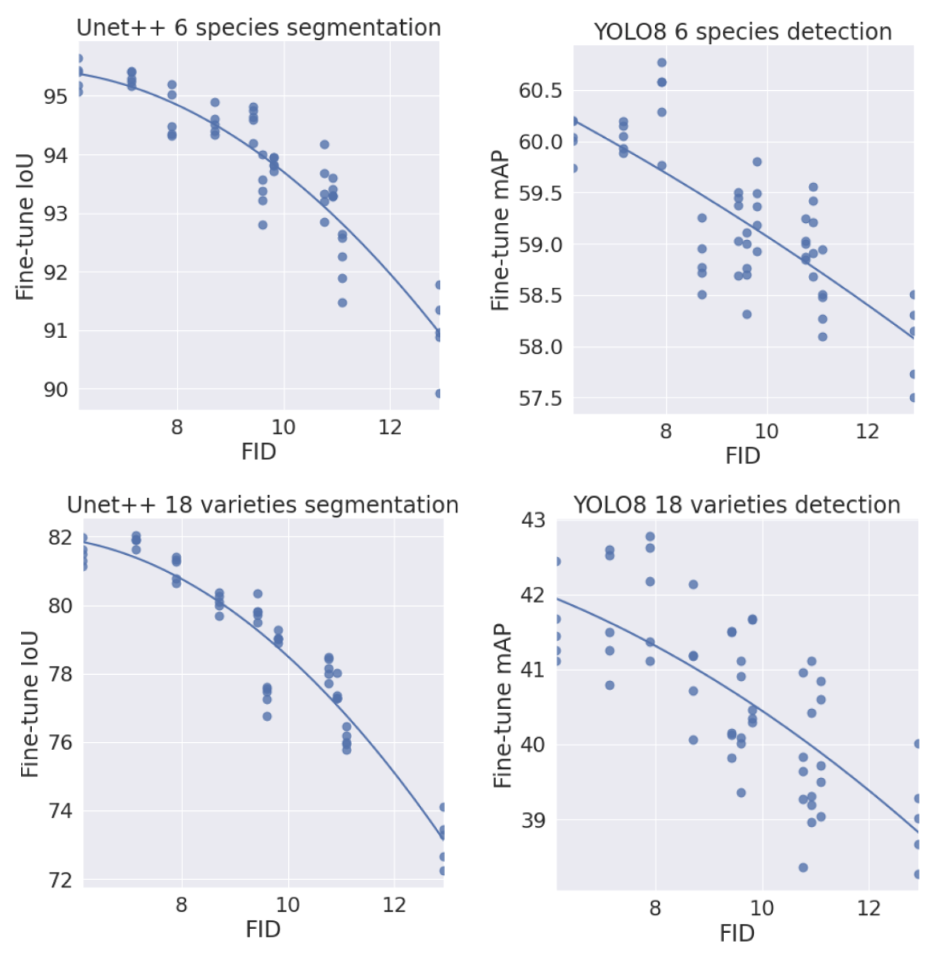
Table 15 as well as
Figure 9 and
Figure 10 show the correlation between the model performance and FID. One can see that if an augmented training set is similar to the test set, it will result in higher accuracy. It allows for choosing a better set of backgrounds without model training. For more complex tasks, the correlation seems to be lower. For segmentation and detection tasks, the correlation is very high.
The importance of context for image augmentation has been previously demonstrated in [
37], where the authors created an additional neural network to select a proper location on a new background to paste the target object. In turn, we focus on the retrieval and generation of an extensive dataset using various sources of background images. Although the proposed approach does not involve additional generative models for dataset augmentation, it is a simple and powerful way to adjust recognition model performance. CISA instance-level augmentation extends the pioneering research on image augmentation [
35] and recent studies [
36], and it allows one to estimate dataset suitability before model training based on FID measures between original and generated datasets.
4.2. Limitations
The proposed image augmentation scheme can be used when we have masks for input images. The system can work with instance segmentation masks and semantic segmentation masks. However, if there are no instance masks available, one can try to generate pseudo-segmentation masks.
The system’s primary usage involves generating complex scenes from simple input data; however, the scene can include a single object if needed. The key feature of the system is its ability to generate a huge amount of training samples even for the task for which the original dataset was not designed. For instance, having only an image and a multi-part mask as input, we can produce samples for instance segmentation, instance parts segmentation, object detection, object counting, denoising, and classification. The described system can also be beneficial for few-shot learning when the original dataset is minimal.
To apply the proposed augmentation scheme successfully, the dataset should not be exceedingly sensitive to scene geometry, since such behavior can be undesirable in some cases. For example, if you use a dataset of people or cars, the described approach by default can place one object on top of the other. Nevertheless, we can add some extra height limitations or use perspective transformation in these cases.
Another point is that we should find appropriate background images that would fit some particular case. Retrieval-based approaches used to generate new training samples using CLIP can be significantly impeded, in particular, domains such as medical or remote sensing. For instance, in [
43], the authors aimed to generate thermal images, with defective areas occurring due to the manufacturing process. It is a more complex task to retrieve such unique backgrounds using CLIP. However, there are various special data sources that do not contain annotated data but are useful as backgrounds for new samples. Another possible limitation is that if it is not possible to know the test set context, we may expect a slight performance drop.
Further study on CISA application for images derived from different sensors on different wavelengths should be conducted. Multispectral and hyperspectral data, radiography, and radar scanning have their own properties. Their artificial generation is currently under consideration in a number of works [
61]. However, it is vital to take into account the nature of data, because image augmentations should not break any physical law of the studied objects.
Recall that it is important to fine-tune the model on natural images to increase the performance.
The time for scene generation is close to linear when we have enough memory to store all objects and overhead for a scene. To estimate the average required RAM per scene, we use Equation (
9)
In this equation, we can neglect the overhead, , because it is considerably smaller than the data itself.
Although GAN-based image augmentation approaches are capable of providing more realistic images under certain conditions, the proposed CISA approach does not require computational resources to train an additional generative model.


 ,
, 


