Quiescent Optical Solitons for the Concatenation Model with Nonlinear Chromatic Dispersion

Abstract

This paper recovers quiescent optical solitons that are self-sustaining, localized wave packets that maintain their shape and amplitude over long distances due to a balance between nonlinearity and dispersion. When a soliton is in a state of quiescence, it means that it is stationary in both space and time. Quiescent optical solitons are typically observed in optical fibers, where nonlinearity and dispersion can lead to the formation of solitons. The concatenation model is considered to understand the behavior of optical pulses propagating through nonlinear media. Here, we consider the familiar nonlinear Schrödinger equation, the Lakshmanan–Porsezian–Daniel equation, and the Sasa–Satsuma equation. The current paper also addresses the model with nonlinear chromatic dispersion, a phenomenon that occurs in optical fibers and other dispersive media, where the chromatic dispersion of the material is modified by nonlinear effects. In the presence of nonlinearities, such as self-phase modulation and cross-phase modulation, the chromatic dispersion coefficient becomes a function of the optical intensity, resulting in nonlinear chromatic dispersion. A full spectrum of stationary optical solitons, along with straddled stationary solitons, are obtained. There are four integration schemes that made this retrieval possible. The numerical simulations are also included for these solitons. The parameter constraints also indicate the existence criteria for these quiescent solitons.

1. Introduction

Optical solitons are self-sustaining, nonlinear waves that propagate in optical fibers or other dispersive media. They are characterized by their ability to maintain their shape and velocity over long distances, without spreading out or dissipating their energy, and can be used for long-distance communication and information processing. To understand optical solitons, it is important to first understand dispersion. In optics, dispersion refers to the phenomenon where different frequencies of light travel at different speeds in a medium. This causes the different frequencies to spread out and interfere with each other, leading to distortion and loss of signal. Optical solitons arise when the effects of dispersion are balanced by nonlinear effects, such as self-phase modulation, four-wave mixing, and stimulated Raman scattering. These nonlinear effects cause the different frequencies of light to interact with each other, leading to the formation of a solitary wave packet that can propagate over long distances without spreading out or dissipating its energy. The shape of an optical soliton depends on the balance between the dispersion and nonlinear effects. If the nonlinear effects are stronger than the dispersion, the soliton is “self-compressed”, with a narrow, high-intensity peak. If the dispersion is stronger than the nonlinear effects, the soliton is “self-expanded”, with a wider, lower-intensity peak. One of the key features of optical solitons is their ability to “heal”, after encountering disturbances or perturbations. This is due to the soliton’s nonlinear properties, which allow it to self-adjust and maintain its shape and velocity. As a result, optical solitons can be used for long-distance communication and information processing in optical fiber networks. There are different types of optical solitons, such as bright solitons, dark solitons, and soliton trains. Bright solitons are characterized by a narrow, high-intensity peak, while dark solitons have a narrow, low-intensity peak surrounded by a wider, higher-intensity background. Soliton trains are a series of solitons that propagate together, separated by small gaps.

Hasegawa and Tappert reported on an optical soliton burning bright fifty years after its first appearance. There exists a wide variety of models that govern the study of such solitons through diverse forms of waveguides. These models provide a mathematical description of the behavior of optical solitons, which is important for understanding and predicting their behavior in different types of nonlinear media. Almost a decade ago a new model was proposed that is a concatenated version of the familiar nonlinear Schrödinger’s equation (NLSE), Lakshmanan–Porsezian–Daniel (LPD) equation and the Sasa–Satsuma equation (SSE). This is being referred to as the concatenation model [1,2], where the NLSE is, perhaps, the most commonly used equation to describe the behavior of solitons in a wide range of physical systems, including optical fibers. The LPD equation is a modification of the NLSE that includes higher-order nonlinear effects. The SS equation is another modified form of the NLSE that includes higher-order nonlinear effects. All of these equations are important tools for understanding the behavior of optical solitons in nonlinear media. By solving these equations, researchers can gain insights into the properties of solitons, including their stability, interactions, and propagation characteristics.

The concatenation model was studied extensively in 2022 and a plethora of results reported. These results included the recovery of single bright, dark and singular optical solitons using the following methods: undetermined coefficients, the conservation laws, Painleve analysis, numerical simulation using the Laplace–Adomian decomposition scheme, and further analytical studies to the model conducted using the trial equation approach. A bright optical soliton is a self-trapped pulse with a positive amplitude that maintains its shape and intensity while propagating through a nonlinear medium. Bright solitons have a maximum in the center of the pulse and are created through the process of soliton compression. A dark optical soliton is a self-trapped pulse with a negative amplitude that maintains its shape and intensity while propagating through a nonlinear medium. Dark solitons have a minimum in the center of the pulse and are created through the process of soliton fission. Singular optical solitons are localized waves that are characterized by a phase singularity or vortex. They can have either bright or dark intensity profiles, depending on the sign of the singularity. Singular optical solitons are created through the process of phase engineering, which involves shaping the phase profile of an input beam to create a phase singularity.

Mobile straddled solitons with the concatenation model were also obtained by the usage of a couple of integration schemes [2,3,4,5,6,7,8]. The current paper aimed to study and recover the quiescent optical solitons for this concatenation model using four integration schemes. This recovery is possible when chromatic dispersion (CD) is rendered to be nonlinear. Mobile optical solitons are solitons that move through a medium without changing their shape or amplitude. They maintain their stability and can propagate over long distances without distortion. Bright optical solitons are typically mobile solitons, and they are widely used in optical communications. Quiescent optical solitons are solitons that are stationary or nearly stationary. They are created by balancing the nonlinear effects of the medium with the dispersion and losses of the system. When the nonlinear effects are balanced, the soliton comes to rest, resulting in a quiescent soliton. Dark optical solitons are typically quiescent solitons. Mobile solitons are particularly important for high-speed data transmission, while quiescent solitons are useful for generating stable and localized sources of light. The integration procedure and the analytical results for these stationary solitons are exhibited, along with their respective numerical simulations. The parametric restrictions for the existence of such solitons are also presented in the rest of the paper.

Governing Model

The concatenation model takes the form [1,2,3,4,5,6,7,8]:

$$\begin{array}{ccc}& & i{q}_t+a{\left({\left|q\right|}^{n}q\right)}_{xx}+b{\left|q\right|}^{2}q\hfill \\ & +& c_1\left[{\delta }_1{q}_{xxxx}+{\delta }_2{\left(q_x\right)}^2{q}^{\ast }+{\delta }_3{\left|q_x\right|}^{2}q+{\delta }_4{\left|q\right|}^2{q}_{xx}+{\delta }_5{q}^2{q}_{xx}^{\ast }+{\delta }_6{\left|q\right|}^{4}q\right]\hfill \\ & +& i{c}_2\left[{\delta }_7{q}_{xxx}+{\delta }_8{\left|q\right|}^2{q}_x+{\delta }_9{q}^2{q}_x^{\ast }\right]=0.\hfill \end{array}$$

(1)

Taking $c_1=0$ falls back (1) to the SSE, while assuming $c_1=c_2=0$ reduces (1) to the NLSE. Furthermore, taking $c_2=0$ collapses (1) to the LPD model. The $c_1$ and $c_2$ arise from the dispersion terms, while $q=q(x,t)$ stems from the wave profile. The a comes from the nonlinear CD, while the first term signifies the linear temporal evolution. The x and t arise from the spatial and temporal variables in sequence, while b evolves from the Kerr of nonlinearity. The first term on the left-hand side of the equation represents the rate of change of the pulse envelope with respect to distance, while the second term represents the effect of nonlinear chromatic dispersion, which causes different wavelengths of light to propagate at different speeds. The third term represents the effect of nonlinear self-phase modulation, which causes the phase of the pulse to vary with intensity.

Here, the NLSE is a well-known partial differential equation that describes the propagation of nonlinear waves in a variety of physical systems, including optics, water waves, and Bose–Einstein condensates. In optics, the NLSE is widely used to model the behavior of ultrafast optical pulses in fiber optic communication systems. The LPD equation is a modified version of the NLSE that includes higher-order nonlinear effects. It was proposed by Lakshmanan, Porsezian, and Daniel in 1992 as a more accurate model for the propagation of ultrafast optical pulses in fiber optic communication systems. The LPD equation can be used to study a wide range of nonlinear optical phenomena, including soliton propagation, pulse compression, and supercontinuum generation, and it provides a more accurate model than the NLSE for systems with higher-order nonlinear effects. The SSE is another nonlinear equation that is used to model the propagation of optical pulses in dispersive and nonlinear media. It was proposed by Sasa and Satsuma in 1974 and is a modification of the NLSE that includes higher-order nonlinear and dispersive effects. The SSE can be used to study a variety of nonlinear optical phenomena, including soliton propagation, pulse compression, and supercontinuum generation. In particular, the SSE can predict the formation of higher-order solitons, which are self-sustaining wave packets with more complex shapes than the fundamental solitons described by the NLSE. The SSE can also predict the generation of frequency-shifted solitons, which can be used for wavelength conversion and other applications in optical communications.

The stationary soliton profile is assumed to be

$$q(x,t)=U\left(kx\right)e^{i(\omega t+\theta )},$$

(2)

where $\theta$ stems from the phase constant and $\omega$ stems from the wave number. Plugging (2) into (1) yields the real part

$$\begin{gathered} a{k}^{2}n\left(n+1\right)U^n{\left(U^{\prime }\right)}^2+a{k}^2\left(n+1\right)U^{1+n}{U}^{″}+c_1{k}^2\left({\delta }_2+{\delta }_3\right){\left(U^{\prime }\right)}^2{U}^2 \\ +c_1{k}^2\left({\delta }_4+{\delta }_5\right)U^3{U}^{″}+c_1{\delta }_1{k}^4{U}^{\left(iv\right)}U-\omega U^2+b{U}^4+c_1{\delta }_6{U}^6=0, \end{gathered}$$

(3)

and the imaginary part

$$c_2{\delta }_7{U}^{‴}U{k}^3+c_{2}k\left({\delta }_8+{\delta }_9\right)U^3{U}^{\prime }=0.$$

(4)

For integrability, one requires

$$n=2,$$

(5)

$${\delta }_7=0,$$

(6)

and

$${\delta }_8+{\delta }_9=0.$$

(7)

After implementing these, the governing Equation (1) modifies to:

$$\begin{array}{ccc}& & i{q}_t+a{\left({\left|q\right|}^{2}q\right)}_{xx}+b{\left|q\right|}^{2}q\hfill \\ & +& c_1\left[{\delta }_1{q}_{xxxx}+{\delta }_2{\left(q_x\right)}^2{q}^{\ast }+{\delta }_3{\left|q_x\right|}^{2}q+{\delta }_4{\left|q\right|}^2{q}_{xx}+{\delta }_5{q}^2{q}_{xx}^{\ast }+{\delta }_6{\left|q\right|}^{4}q\right]+i{c}_2\left[{\delta }_8{\left|q\right|}^2{q}_x+{\delta }_9{q}^2{q}_x^{\ast }\right]=0.\hfill \end{array}$$

(8)

Then, Equation (3) reduces to:

$$c_1{\delta }_1{k}^4{U}^{\left(iv\right)}+\left[3a{k}^2+c_1{k}^2\left({\delta }_4+{\delta }_5\right)\right]U^2{U}^{″}+\left[6a{k}^2+c_1{k}^2\left({\delta }_2+{\delta }_3\right)\right]U{\left(U^{\prime }\right)}^2-\omega U+b{U}^3+c_1{\delta }_6{U}^5=0.$$

(9)

2. Review of Implemented Integration Algorithms

Consider the model equation

$$G(q,q_x,q_t,q_{xt},q_{xx},\dots )=0,$$

(10)

where $q=q(x,t)$ is the optoelectronic wave field, while x and t are spatial and temporal variables.

Set the certain restrictions

$$q(x,t)=U\left(\xi \right),\xi =\mu (x-vt),$$

(11)

where v is the wave velocity, $\xi$ is the wave variable and $\mu$ is the wave width. Thus, (10) falls out as

$$P(U,-\mu \upsilon U^{\prime },\mu U^{\prime },{\mu }^2{U}^{″},...)=0.$$

(12)

2.1. Sine–Gordon Equation Scheme

Step–1: The theoretical model (12) permits the solution form [9]

$$U\left(\xi \right)=\sum _{i=1}^N{cos}^{i-1}\left(F\left(\xi \right)\right)\left[B_{i}sin\left(F\left(\xi \right)\right)+C_{i}cos\left(F\left(\xi \right)\right)\right]+C_0,$$

(13)

along with the auxiliary equation

$$F^{\prime }\left(\xi \right)=sin\left(F\left(\xi \right)\right),$$

(14)

which holds the soliton wave structures

$$sin\left(F\left(\xi \right)\right)=\mathrm{sech}\left(\xi \right)\mathrm{or}sin\left(F\left(\xi \right)\right)=i\mathrm{csch}\left(\xi \right),$$

(15)

and

$$cos\left(F\left(\xi \right)\right)=\tanh \left(\xi \right)\mathrm{or}cos\left(F\left(\xi \right)\right)=\coth \left(\xi \right),$$

(16)

where $C_0$, $C_i$ and $B_i$$(i=0,1,\cdots ,N)$ are constants, while N comes from the balancing algorithm in (12).

Step–2: Substituting (13), along with (14), into (12), we obtain a polynomial expression in terms of $cos\left(F\left(\xi \right)\right)$ and $sin\left(F\left(\xi \right)\right)$. We then collect all terms with the same powers and set them equal to zero, resulting in an over-determined system of algebraic equations. This system can be solved using software such as Maple or Mathematica to obtain the unknown parameters. Once these parameters are found, we substitute them, along with Equations (15) and (16), back into Equation (13) to obtain the nonlinear wave profiles.

2.2. F–Expansion Procedure

Step–1: The simplified model (12) satisfies the solution structure [10]

$$U\left(\xi \right)=\sum _{i=0}^N{B}_i{F}^i\left(\xi \right),$$

(17)

with the aid of the ancillary equation

$$F^{\prime }\left(\xi \right)=\sqrt{P{F}^4\left(\xi \right)+Q{F}^2\left(\xi \right)+R},$$

(18)

which leaves us with the soliton wave profiles

$$F\left(\xi \right)=\mathrm{sn}\left(\xi \right)=\tanh \left(\xi \right),P=m^2,Q=-(1+m^2),R=1,m\to 1^{-},$$

(19)

$$F\left(\xi \right)=\mathrm{ns}\left(\xi \right)=\coth \left(\xi \right),P=1,Q=-(1+m^2),R=m^2,m\to 1^{-},$$

(20)

$$F\left(\xi \right)=\mathrm{cn}\left(\xi \right)=\mathrm{sech}\left(\xi \right),P=-m^2,Q=2m^2-1,R=1-m^2,m\to 1^{-},$$

(21)

$$F\left(\xi \right)=\mathrm{ds}\left(\xi \right)=\mathrm{csch}\left(\xi \right),P=1,Q=2m^2-1,R=-m^2\left(1-m^2\right),m\to 1^{-},$$

(22)

$$F\left(\xi \right)=\mathrm{ns}\left(\xi \right)\pm \mathrm{ds}\left(\xi \right)=coth\left(\xi \right)\pm \mathrm{csch}\left(\xi \right),P=\frac{1}{4},Q=\frac{m^2-2}{2},R=\frac{m^2}{4},m\to 1^{-},$$

(23)

and

$$F\left(\xi \right)=\mathrm{sn}\left(\xi \right)\pm \mathrm{icn}\left(\xi \right)=tanh\left(\xi \right)\pm \mathrm{i}\mathrm{sech}\left(\xi \right),P=\frac{m^2}{4},Q=\frac{m^2-2}{2},R=\frac{m^2}{4},m\to 1^{-},$$

(24)

where sn$\left(\xi \right)$, ns$\left(\xi \right)$, cn$\left(\xi \right)$ and ds$\left(\xi \right)$ are the Jacobi’s elliptic functions (JEFs), while $0<m<1$ is the modulus of the JEFs. $B_i$$(i=0,1,\cdots ,N)$ are constants, while N stems from the balancing approach in (12).

Step–2: Inserting (17), together with (18), into (12), we obtain a polynomial in $F\left(\xi \right)$. We then group terms of the same powers and set each group equal to zero. This results in an over-determined system of algebraic equations, which can be solved using software such as Maple or Mathematica. Solving these equations yields the values of the unknown parameters. Substituting these parameters, along with Equations (19)–(24), into Equation (17) gives us the optoelectronic wave fields.

2.3. Riccati Equation Method

Step–1: The theoretical model (12) permits the solution form [11]

$$U\left(\xi \right)=\sum _{i=0}^N{A}_i{V}^i\left(\xi \right),$$

(25)

along with the auxiliary equation

$$V^{\prime }\left(\xi \right)=S_2{V}^2\left(\xi \right)+S_{1}V\left(\xi \right)+S_0,S_2\ne 0,$$

(26)

which holds the soliton wave structures

$$V\left(\xi \right)=-\frac{S_1}{2S_2}-\frac{\sqrt{\rho }}{2S_2}tanh\left(\frac{\sqrt{\rho }}{2}\xi +{\xi }_0\right),\rho >0,$$

(27)

and

$$V\left(\xi \right)=-\frac{S_1}{2S_2}-\frac{\sqrt{\rho }}{2S_2}coth\left(\frac{\sqrt{\rho }}{2}\xi +{\xi }_0\right),\rho >0,$$

(28)

where $S_0$, $S_1$, $S_2$ and ${\xi }_0$ are constants and $\rho =$$S_1^2-4S_0{S}_2$, while N comes from the balancing algorithm in (12).

Step–2: Plugging (25), along with (26), into (12), we obtain a polynomial expression in terms of $V\left(\xi \right)$. We then collect all terms with the same powers and set them equal to zero, resulting in an over-determined system of algebraic equations. This system can be solved using software such as Maple or Mathematica to obtain the unknown parameters. Once these parameters are found, we substitute them, along with Equations (27) and (28), back into Equation (25) to obtain the nonlinear waveforms.

2.4. Extended Jacobi’s Elliptic Function Expansion

Step–1: The simplified model (12) satisfies the solution structure [12]

$$U\left(\xi \right)=\sum _{i=0}^N{A}_i{\mathrm{sn}}^i\left(\xi \right)+\sum _{i=1}^N{B}_i{\mathrm{sn}}^{-i}\left(\xi \right),$$

(29)

with the aid of the ancillary equations

$${\mathrm{cn}}^2\left(\xi \right)=1-{\mathrm{sn}}^2\left(\xi \right),$$

(30)

$${\mathrm{dn}}^2\left(\xi \right)=1-l^2{\mathrm{sn}}^2\left(\xi \right),$$

(31)

$$\frac{d}{d\xi }\mathrm{sn}\left(\xi \right)=\mathrm{cn}\left(\xi \right)\mathrm{dn}\left(\xi \right),$$

(32)

$$\frac{d}{d\xi }\mathrm{cn}\left(\xi \right)=-\mathrm{sn}\left(\xi \right)\mathrm{dn}\left(\xi \right),$$

(33)

and

$$\frac{d}{d\xi }\mathrm{dn}\left(\xi \right)=-l^2\mathrm{sn}\left(\xi \right)\mathrm{cn}\left(\xi \right),$$

(34)

which leaves us with the soliton wave profiles

$$\mathrm{sn}\left(\xi \right)=tanh\left(\xi \right),l\to 1^{-},$$

(35)

and

$${\mathrm{sn}}^{-1}\left(\xi \right)=coth\left(\xi \right),l\to 1^{-},$$

(36)

where sn$\left(\xi \right)$, cn$\left(\xi \right)$ and dn$\left(\xi \right)$ are the JEFs, while $0<l<1$ is the modulus of the JEFs. $A_i$ and $B_i$$(i=0,1,\cdots ,N)$ are constants, while N stems from the balancing approach in (12).

Step–2: Putting (29), together with (30)–(34), into (12), we obtain a polynomial in sn$\left(\xi \right)$, cn$\left(\xi \right)$ and dn$\left(\xi \right)$. We then group terms of the same powers and set each group equal to zero. This results in an over-determined system of algebraic equations, which can be solved using software such as Maple or Mathematica. Solving these equations yields the values of the unknown parameters. Substituting these parameters, along with Equations (35) and (36), into Equation (29) gives us the soliton wave profiles.

3. Quiescent Optical Solitons

Quiescent optical solitons are a type of soliton that arise in nonlinear optical systems with competing nonlinearities. Unlike traditional optical solitons, which propagate at a constant velocity and maintain their shape over long distances, quiescent optical solitons are stationary and have a nontrivial shape. Quiescent solitons have been observed experimentally in a variety of nonlinear optical systems, including optical fibers, photonic lattices, and waveguide arrays. They have also been studied theoretically using models such as the nonlinear Schrödinger equation with competing nonlinearities and the Gross–Pitaevskii equation for Bose–Einstein condensates. Quiescent solitons have unique properties compared to traditional solitons. A quiescent soliton has a broader spectrum, and a shape that is less robust to perturbations due to having lower intensity in the central region. However, they have been shown to have advantages in applications, such as pulse compression and optical switching. Quiescent optical solitons can be classified into several types based on their properties, for which we offer brief descriptions of some of the types. Quiescent optical bright solitons have a localized peak in the intensity of the optical pulse. They are characterized by a central region of high intensity surrounded by lower intensity regions. Quiescent optical dark solitons have a localized dip in the intensity of the optical pulse. They are characterized by a central region of low intensity surrounded by higher intensity regions. Quiescent optical singular solitons have a sharp point or cusp in the intensity profile. They are sometimes referred to as “kinks” or “peaks”. Quiescent optical straddled solitons have two peaks separated by a dip in the intensity profile. They are characterized by a central region of low intensity surrounded by two regions of high intensity.

In this section, the four integration strategies are implemented to secure quiescent optical solitons for the model. To this end, balancing the terms $U^{\left(iv\right)}$ with $U^5$ in (9) yields $N=1$. The procedures are organized in the coming subsections.

3.1. Sine–Gordon Equation Method

In this integration tool, the formal solution structure (13) condenses to

$$U\left(\xi \right)=B_{1}sin\left(F\left(\xi \right)\right)+C_{1}cos\left(F\left(\xi \right)\right)+C_0.$$

(37)

Inserting (37), along with (14), into (9), the auxiliary equations are enlisted as:

$$\begin{gathered} b{B_1}^3-\omega B_1+k^2{B}_1{C_1}^2{c}_1{\delta }_2+k^2{B}_1{C_1}^2{c}_1{\delta }_3-k^2{B_1}^3{c}_1{\delta }_4-k^2{B_1}^3{c}_1{\delta }_5 \\ +5k^4{B}_1{c}_1{\delta }_1+6a{k}^2{B}_1{C_1}^2-3a{k}^2{B_1}^3+{B_1}^5{c}_1{\delta }_6=0, \end{gathered}$$

(38)

$$\begin{gathered} -\omega C_1-4k^2{B_1}^2{C}_1{c}_1{\delta }_4-4k^2{B_1}^2{C}_1{c}_1{\delta }_5-2k^2{B_1}^2{C}_1{c}_1{\delta }_3-2k^2{B_1}^2{C}_1{c}_1{\delta }_2-24a{k}^2{B_1}^2{C}_1 \\ +16c_1{\delta }_1{k}^4{C}_1+5{B_1}^4{C}_1{c}_1{\delta }_6+k^2{C_1}^3{c}_1{\delta }_2+k^2{C_1}^3{c}_1{\delta }_3+6a{k}^2{C_1}^3+3b{B_1}^2{C}_1=0, \end{gathered}$$

(39)

$$\begin{gathered} -2k^2{B_1}^3{c}_1{\delta }_4-2k^2{B_1}^3{c}_1{\delta }_5-10{B_1}^3{C_1}^2{c}_1{\delta }_6+5B_1{C_1}^4{c}_1{\delta }_6-k^2{B_1}^3{c}_1{\delta }_2 \\ -k^2{B_1}^3{c}_1{\delta }_3+24k^4{B}_1{c}_1{\delta }_1+36a{k}^2{B}_1{C_1}^2+{B_1}^5{c}_1{\delta }_6-12a{k}^2{B_1}^3+3k^2{B}_1{C_1}^2{c}_1{\delta }_2 \\ +6k^2{B}_1{C_1}^2{c}_1{\delta }_4+6k^2{B}_1{C_1}^2{c}_1{\delta }_5+3k^2{B}_1{C_1}^2{c}_1{\delta }_3=0, \end{gathered}$$

(40)

$$\begin{gathered} -10{B_1}^2{C_1}^3{c}_1{\delta }_6+5{B_1}^4{C}_1{c}_1{\delta }_6+{C_1}^5{c}_1{\delta }_6-3k^2{B_1}^2{C}_1{c}_1{\delta }_2-3k^2{B_1}^2{C}_1{c}_1{\delta }_3 \\ -6k^2{B_1}^2{C}_1{c}_1{\delta }_4-6k^2{B_1}^2{C}_1{c}_1{\delta }_5+24c_1{\delta }_1{k}^4{C}_1+2k^2{C_1}^3{c}_1{\delta }_4+2k^2{C_1}^3{c}_1{\delta }_5 \\ -36a{k}^2{B_1}^2{C}_1+k^2{C_1}^3{c}_1{\delta }_2+k^2{C_1}^3{c}_1{\delta }_3+12a{k}^2{C_1}^3=0, \end{gathered}$$

(41)

$$\begin{gathered} b{C_1}^3+5k^2{B_1}^2{C}_1{c}_1{\delta }_2+5k^2{B_1}^2{C}_1{c}_1{\delta }_3+10k^2{B_1}^2{C}_1{c}_1{\delta }_4+10k^2{B_1}^2{C}_1{c}_1{\delta }_5 \\ -10{B_1}^4{C}_1{c}_1{\delta }_6+10{B_1}^2{C_1}^3{c}_1{\delta }_6+60a{k}^2{B_1}^2{C}_1-2k^2{C_1}^3{c}_1{\delta }_2-2k^2{C_1}^3{c}_1{\delta }_3 \\ -40c_1{\delta }_1{k}^4{C}_1-2k^2{C_1}^3{c}_1{\delta }_4-2k^2{C_1}^3{c}_1{\delta }_5-3b{B_1}^2{C}_1-18a{k}^2{C_1}^3=0, \end{gathered}$$

(42)

$$\begin{gathered} 10{B_1}^3{C_1}^2{c}_1{\delta }_6+k^2{B_1}^3{c}_1{\delta }_2+k^2{B_1}^3{c}_1{\delta }_3-28k^4{B}_1{c}_1{\delta }_1+3k^2{B_1}^3{c}_1{\delta }_4 \\ +3k^2{B_1}^3{c}_1{\delta }_5-39a{k}^2{B}_1{C_1}^2+3b{B}_1{C_1}^2-2{B_1}^5{c}_1{\delta }_6+15a{k}^2{B_1}^3-4k^2{B}_1{C_1}^2{c}_1{\delta }_3 \\ -4k^2{B}_1{C_1}^2{c}_1{\delta }_2-5k^2{B}_1{C_1}^2{c}_1{\delta }_4-5k^2{B}_1{C_1}^2{c}_1{\delta }_5-b{B_1}^3=0. \end{gathered}$$

(43)

On solving these equations, one retrieves the following results:

Result–1:

$${\delta }_6=\frac{\left(2k^2{c}_1{\delta }_2+2k^2{c}_1{\delta }_3+2k^2{c}_1{\delta }_4+2k^2{c}_1{\delta }_5+18a{k}^2-b\right)\left(-k^2{c}_1{\delta }_2-k^2{c}_1{\delta }_3+4k^2{c}_1{\delta }_4+4k^2{c}_1{\delta }_5+6a{k}^2+3b\right)}{200k^4{c_1}^2{\delta }_1},$$

$$\omega =\frac{8{\delta }_1{c}_1\left(-k^2{c}_1{\delta }_2-k^2{c}_1{\delta }_3+4k^2{c}_1{\delta }_4+4k^2{c}_1{\delta }_5+6a{k}^2-2b\right)k^4}{2k^2{c}_1{\delta }_2+2k^2{c}_1{\delta }_3+2k^2{c}_1{\delta }_4+2k^2{c}_1{\delta }_5+18a{k}^2-b},$$

$$C_0=0,B_1=0,C_1=\pm 2k^2\sqrt{-\frac{10{\delta }_1{c}_1}{2k^2{c}_1{\delta }_2+2k^2{c}_1{\delta }_3+2k^2{c}_1{\delta }_4+2k^2{c}_1{\delta }_5+18a{k}^2-b}}.$$

(44)

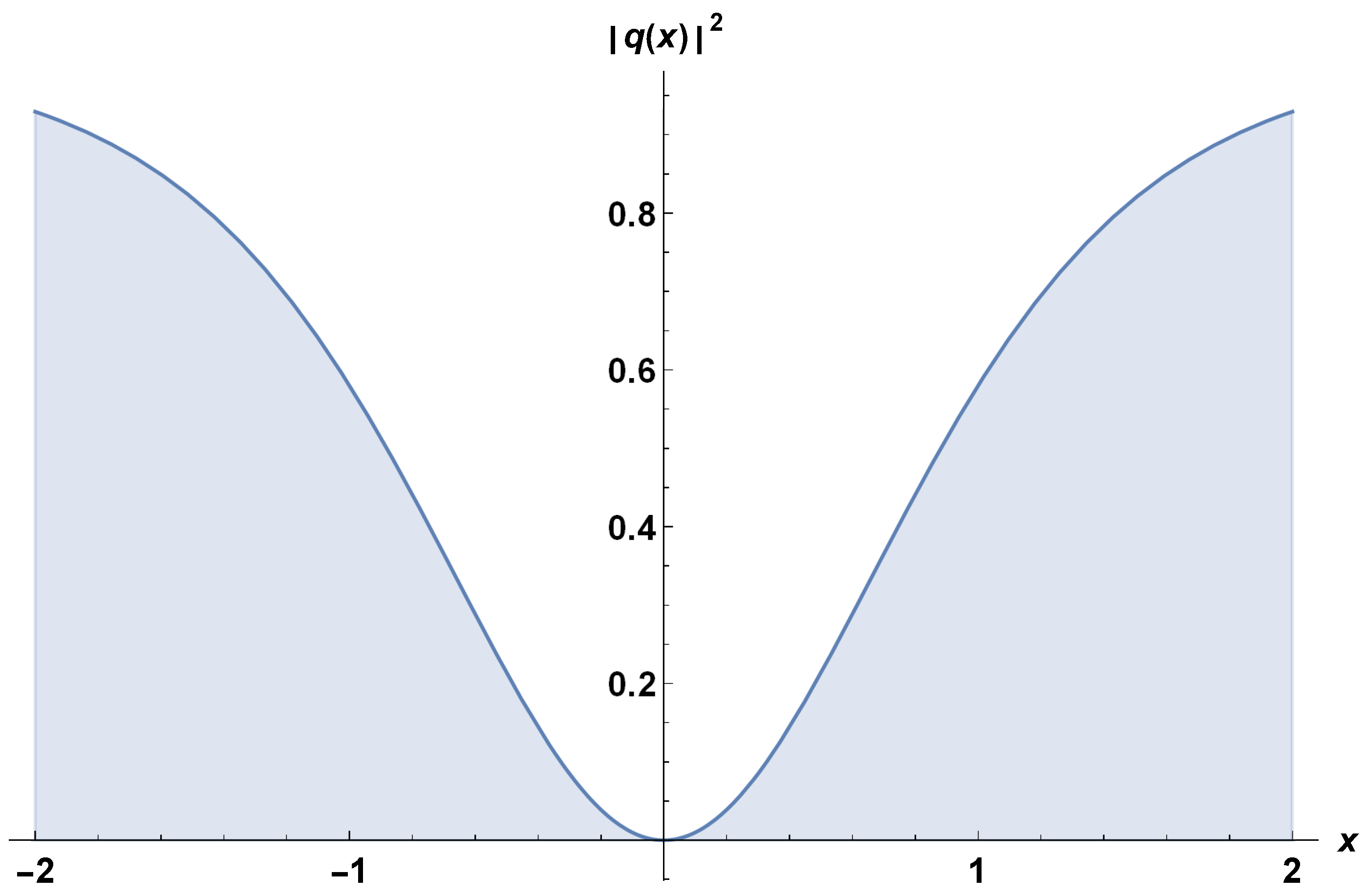
Inserting (44), along with (16) into (37), the quiescent dark and singular optical solitons are presented as indicated below:

$$\begin{array}{ccc}\hfill q(x,t)& =& \pm 2k^2\sqrt{-\frac{10{\delta }_1{c}_1}{2k^2{c}_1{\delta }_2+2k^2{c}_1{\delta }_3+2k^2{c}_1{\delta }_4+2k^2{c}_1{\delta }_5+18a{k}^2-b}}\tanh \left(kx\right)\hfill \\ & & \times e^{i\left({\displaystyle \frac{8{\delta }_1{c}_1\left(-k^2{c}_1{\delta }_2-k^2{c}_1{\delta }_3+4k^2{c}_1{\delta }_4+4k^2{c}_1{\delta }_5+6a{k}^2-2b\right)k^4}{2k^2{c}_1{\delta }_2+2k^2{c}_1{\delta }_3+2k^2{c}_1{\delta }_4+2k^2{c}_1{\delta }_5+18a{k}^2-b}}t+\theta \right)},\hfill \end{array}$$

(45)

and

$$\begin{array}{ccc}\hfill q(x,t)& =& \pm 2k^2\sqrt{-\frac{10{\delta }_1{c}_1}{2k^2{c}_1{\delta }_2+2k^2{c}_1{\delta }_3+2k^2{c}_1{\delta }_4+2k^2{c}_1{\delta }_5+18a{k}^2-b}}\coth \left(kx\right)\hfill \\ & & \times e^{i\left({\displaystyle \frac{8{\delta }_1{c}_1\left(-k^2{c}_1{\delta }_2-k^2{c}_1{\delta }_3+4k^2{c}_1{\delta }_4+4k^2{c}_1{\delta }_5+6a{k}^2-2b\right)k^4}{2k^2{c}_1{\delta }_2+2k^2{c}_1{\delta }_3+2k^2{c}_1{\delta }_4+2k^2{c}_1{\delta }_5+18a{k}^2-b}}t+\theta \right)},\hfill \end{array}$$

(46)

where

$${\delta }_1{c}_1\left(2k^2{c}_1{\delta }_2+2k^2{c}_1{\delta }_3+2k^2{c}_1{\delta }_4+2k^2{c}_1{\delta }_5+18a{k}^2-b\right)<0.$$

(47)

The optoelectronic wave field (45) is depicted in Figure 1. The parameter values chosen were: $k=1$, $c_1=1$, ${\delta }_2=1$, ${\delta }_3=1$, ${\delta }_4=1$, ${\delta }_5=1$, $a=1$, $b=1$ and ${\delta }_1=-1$. Figure 1 shows a localized dip, or trough, in intensity at the center of the wave pattern. The surrounding wave pattern is characterized by an increase in intensity towards the edges, creating a ring-like, or circular, shape around the dark spot. The dark spot appears as a self-contained entity, maintaining its shape and size as it propagates through the medium.

Result–2:

$$\omega =k^4{c}_1{\delta }_1,B_1=\pm 2k^2\sqrt{\frac{5{\delta }_1{c}_1}{k^2{c}_1{\delta }_2+k^2{c}_1{\delta }_3+k^2{c}_1{\delta }_4+k^2{c}_1{\delta }_5+9a{k}^2+b}},C_1=0,C_0=0,$$

$$3{\delta }_6^4{B_1}^4{c}_1+\left(k^2{c}_1{\delta }_2+k^2{c}_1{\delta }_3-2k^2{c}_1{\delta }_4-2k^2{c}_1{\delta }_5+4b\right){B_1}^2-8k^4{c}_1{\delta }_1=0.$$

(48)

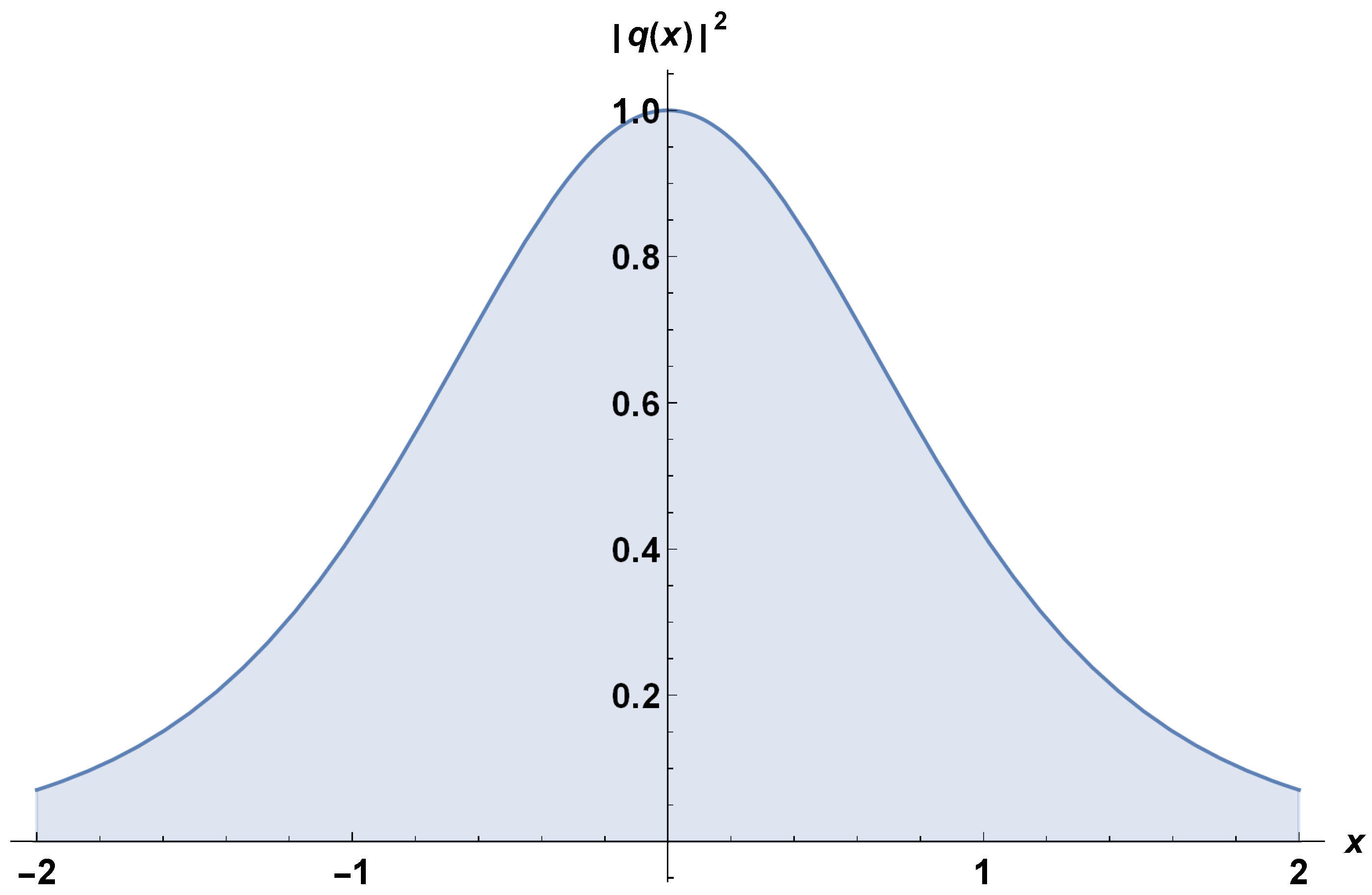
Inserting (48), along with (15), into (37), the bright soliton wave is recovered as:

$$q(x,t)=\pm 2\sqrt{\frac{5{\delta }_1{c}_1}{k^2{c}_1{\delta }_2+k^2{c}_1{\delta }_3+k^2{c}_1{\delta }_4+k^2{c}_1{\delta }_5+9a{k}^2+b}}\mathrm{sech}\left(kx\right)e^{i\left(k^4{c}_1{\delta }_{1}t+\theta \right)},$$

(49)

with the parameter constraints

$${\delta }_1{c}_1\left(k^2{c}_1{\delta }_2+k^2{c}_1{\delta }_3+k^2{c}_1{\delta }_4+k^2{c}_1{\delta }_5+9a{k}^2+b\right)>0.$$

(50)

The singular nonlinear wave profile is also defined as

$$q(x,t)=\pm 2\sqrt{-\frac{5{\delta }_1{c}_1}{k^2{c}_1{\delta }_2+k^2{c}_1{\delta }_3+k^2{c}_1{\delta }_4+k^2{c}_1{\delta }_5+9a{k}^2+b}}\mathrm{csch}\left(kx\right)e^{i\left(k^4{c}_1{\delta }_{1}t+\theta \right)},$$

(51)

with the parameters criteria

$${\delta }_1{c}_1\left(k^2{c}_1{\delta }_2+k^2{c}_1{\delta }_3+k^2{c}_1{\delta }_4+k^2{c}_1{\delta }_5+9a{k}^2+b\right)<0.$$

(52)

The optical nonlinear waveform (49) is portrayed in Figure 2. The parameter values chosen were: $k=1$, $c_1=1$, ${\delta }_2=1$, ${\delta }_3=1$, ${\delta }_4=1$, ${\delta }_5=1$, $a=1$, $b=1$ and ${\delta }_1=1$. Figure 2 typically shows a localized bright spot, or peak, in the center of the wave pattern. The surrounding wave pattern is characterized by a decay in intensity towards the edges, creating a ring-like, or circular, shape around the bright spot. The bright spot appears as a self-contained entity, maintaining its shape and size as it propagates through the medium.

Result–3:

$$k=\pm \frac{2}{5}\sqrt{-\frac{5b}{c_1{\delta }_4+c_1{\delta }_5+3a}},\omega =-\frac{176b^2{c}_1{\delta }_1}{225{\left(c_1{\delta }_4+c_1{\delta }_5+3a\right)}^2},$$

$$B_1=\pm \frac{2}{3}\frac{\sqrt{-22b{c}_1{\delta }_1}}{c_1{\delta }_4+c_1{\delta }_5+3a},C_1=\pm \frac{2}{3}\frac{\sqrt{-2b{c}_1{\delta }_1}}{c_1{\delta }_4+c_1{\delta }_5+3a},C_0=0,$$

$${\delta }_2=-\frac{c_1{\delta }_3-c_1{\delta }_4-c_1{\delta }_5+3a}{c_1},{\delta }_6=\frac{27{\left(c_1{\delta }_4+c_1{\delta }_5+3a\right)}^2}{200{c_1}^2{\delta }_1}.$$

(53)

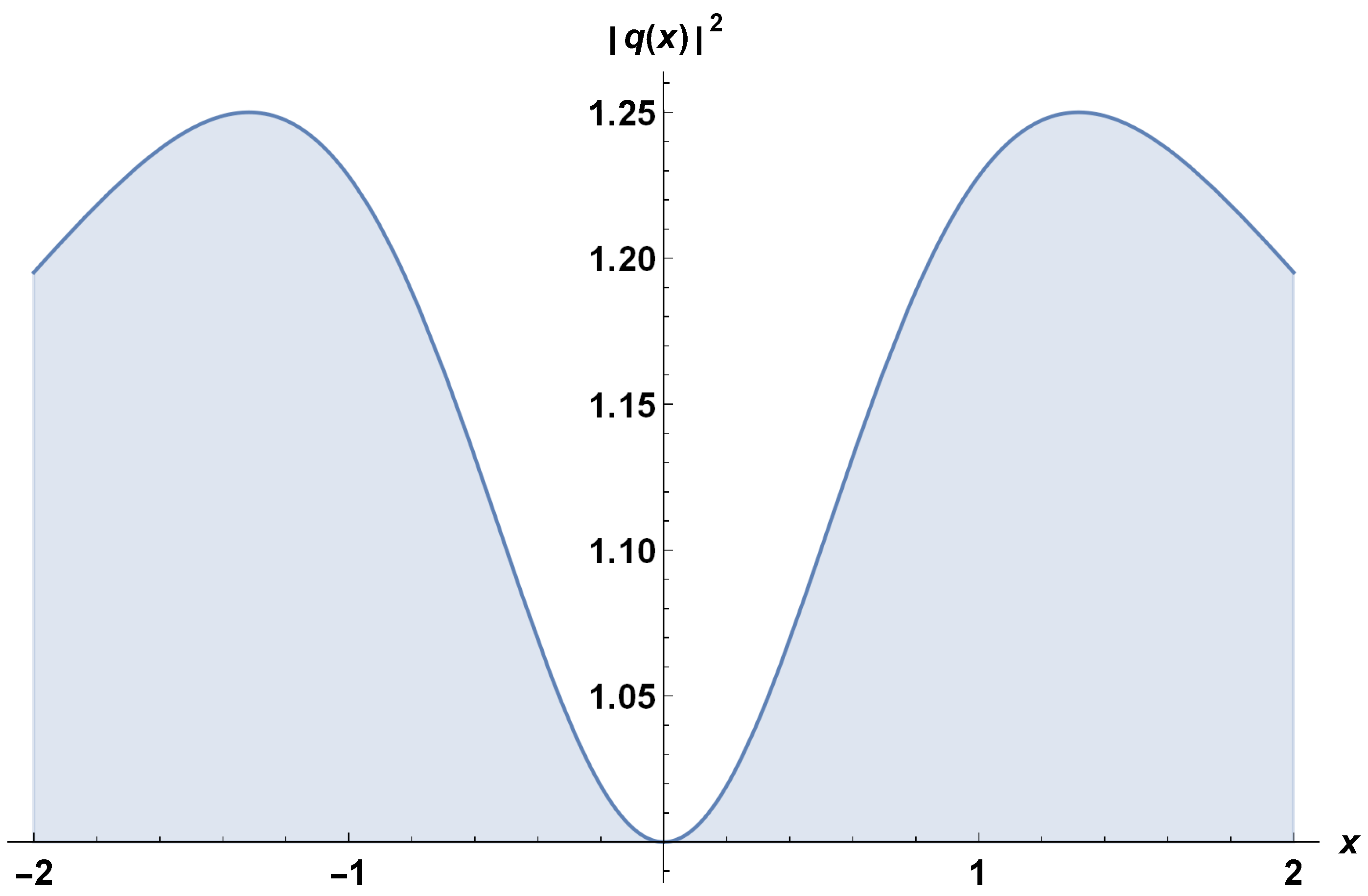
Substituting (53), along with (15) and (16), into (37), the straddled quiescent bright–singular and bright–dark soliton profiles are extracted as

$$\begin{array}{ccc}\hfill q(x,t)& =& \left\{\begin{array}{c}\pm {\displaystyle \frac{2}{3}}{\displaystyle \frac{\sqrt{-22b{c}_1{\delta }_1}}{c_1{\delta }_4+c_1{\delta }_5+3a}}\mathrm{sech}\left(\pm {\displaystyle \frac{2}{5}}\sqrt{-{\displaystyle \frac{5b}{c_1{\delta }_4+c_1{\delta }_5+3a}}}x\right)\\ \pm {\displaystyle \frac{2}{3}}{\displaystyle \frac{\sqrt{-2b{c}_1{\delta }_1}}{c_1{\delta }_4+c_1{\delta }_5+3a}}\coth \left(\pm {\displaystyle \frac{2}{5}}\sqrt{-{\displaystyle \frac{5b}{c_1{\delta }_4+c_1{\delta }_5+3a}}}x\right)\end{array}\right\}\hfill \\ & & \times e^{i\left(-{\displaystyle \frac{176b^2{c}_1{\delta }_1}{225{\left(c_1{\delta }_4+c_1{\delta }_5+3a\right)}^2}}t+\theta \right)},\hfill \end{array}$$

(54)

and

$$\begin{array}{ccc}\hfill q(x,t)& =& \left\{\begin{array}{c}\pm {\displaystyle \frac{2}{3}}{\displaystyle \frac{\sqrt{-22b{c}_1{\delta }_1}}{c_1{\delta }_4+c_1{\delta }_5+3a}}\mathrm{sech}\left(\pm {\displaystyle \frac{2}{5}}\sqrt{-{\displaystyle \frac{5b}{c_1{\delta }_4+c_1{\delta }_5+3a}}}x\right)\\ \pm {\displaystyle \frac{2}{3}}{\displaystyle \frac{\sqrt{-2b{c}_1{\delta }_1}}{c_1{\delta }_4+c_1{\delta }_5+3a}}\tanh \left(\pm {\displaystyle \frac{2}{5}}\sqrt{-{\displaystyle \frac{5b}{c_1{\delta }_4+c_1{\delta }_5+3a}}}x\right)\end{array}\right\}\hfill \\ & & \times e^{i\left(-{\displaystyle \frac{176b^2{c}_1{\delta }_1}{225{\left(c_1{\delta }_4+c_1{\delta }_5+3a\right)}^2}}t+\theta \right)},\hfill \end{array}$$

(55)

with the specific restrictions

$$b{c}_1{\delta }_1<0,$$

(56)

and

$$b\left(c_1{\delta }_4+c_1{\delta }_5+3a\right)>0.$$

(57)

The optical soliton profile (55) is shown in Figure 3. The parameter values chosen were: $c_1=1$, ${\delta }_4=1$, ${\delta }_5=1$, $a=1$, $b=-1$ and ${\delta }_1=1$. Figure 3 shows a localized bright spot flanked by dark troughs on either side. The bright spot propagates through the medium while the dark troughs move at the same speed in the opposite direction. The interaction between the bright and dark regions creates a stable, self-sustaining wave, that can propagate over long distances without changing its shape.

Result–4:

$${\delta }_6=\frac{\left(-k^2{c}_1{\delta }_2-k^2{c}_1{\delta }_3+4k^2{c}_1{\delta }_4+4k^2{c}_1{\delta }_5+6a{k}^2+12b\right)\left(k^2{c}_1{\delta }_2+k^2{c}_1{\delta }_3+k^2{c}_1{\delta }_4+k^2{c}_1{\delta }_5+9a{k}^2-2b\right)}{100k^4{c_1}^2{\delta }_1},$$

$$\omega =\frac{{\delta }_1{c}_1\left(-k^2{c}_1{\delta }_2-k^2{c}_1{\delta }_3+4k^2{c}_1{\delta }_4+4k^2{c}_1{\delta }_5+6a{k}^2-8b\right)k^4}{4\left(k^2{c}_1{\delta }_2+k^2{c}_1{\delta }_3+k^2{c}_1{\delta }_4+k^2{c}_1{\delta }_5+9a{k}^2-2b\right)},$$

$$B_1=\pm i{k}^2\sqrt{-\frac{5{\delta }_1{c}_1}{k^2{c}_1{\delta }_2+k^2{c}_1{\delta }_3+k^2{c}_1{\delta }_4+k^2{c}_1{\delta }_5+9a{k}^2-2b}},C_0=0,$$

$$C_1=\pm k^2\sqrt{-\frac{5{\delta }_1{c}_1}{k^2{c}_1{\delta }_2+k^2{c}_1{\delta }_3+k^2{c}_1{\delta }_4+k^2{c}_1{\delta }_5+9a{k}^2-2b}}.$$

(58)

Plugging (58), together with (15) and (16), into (37), the dark–singular straddled and singular–singular straddled quiescent solitons are respectively structured as

$$\begin{array}{ccc}\hfill q(x,t)& =& \left\{\begin{array}{c}\pm k^2\sqrt{-{\displaystyle \frac{5{\delta }_1{c}_1}{k^2{c}_1{\delta }_2+k^2{c}_1{\delta }_3+k^2{c}_1{\delta }_4+k^2{c}_1{\delta }_5+9a{k}^2-2b}}}\mathrm{csch}\left(kx\right)\\ \pm k^2\sqrt{-{\displaystyle \frac{5{\delta }_1{c}_1}{k^2{c}_1{\delta }_2+k^2{c}_1{\delta }_3+k^2{c}_1{\delta }_4+k^2{c}_1{\delta }_5+9a{k}^2-2b}}}\tanh \left(kx\right)\end{array}\right\}\hfill \\ & & \times e^{i\left({\displaystyle \frac{{\delta }_1{c}_1\left(-k^2{c}_1{\delta }_2-k^2{c}_1{\delta }_3+4k^2{c}_1{\delta }_4+4k^2{c}_1{\delta }_5+6a{k}^2-8b\right)k^4}{4\left(k^2{c}_1{\delta }_2+k^2{c}_1{\delta }_3+k^2{c}_1{\delta }_4+k^2{c}_1{\delta }_5+9a{k}^2-2b\right)}}t+\theta \right)},\hfill \end{array}$$

(59)

and

$$\begin{array}{ccc}\hfill q(x,t)& =& \left\{\begin{array}{c}\pm k^2\sqrt{-{\displaystyle \frac{5{\delta }_1{c}_1}{k^2{c}_1{\delta }_2+k^2{c}_1{\delta }_3+k^2{c}_1{\delta }_4+k^2{c}_1{\delta }_5+9a{k}^2-2b}}}\mathrm{csch}\left(kx\right)\\ \pm k^2\sqrt{-{\displaystyle \frac{5{\delta }_1{c}_1}{k^2{c}_1{\delta }_2+k^2{c}_1{\delta }_3+k^2{c}_1{\delta }_4+k^2{c}_1{\delta }_5+9a{k}^2-2b}}}\coth \left(kx\right)\end{array}\right\}\hfill \\ & & \times e^{i\left({\displaystyle \frac{{\delta }_1{c}_1\left(-k^2{c}_1{\delta }_2-k^2{c}_1{\delta }_3+4k^2{c}_1{\delta }_4+4k^2{c}_1{\delta }_5+6a{k}^2-8b\right)k^4}{4\left(k^2{c}_1{\delta }_2+k^2{c}_1{\delta }_3+k^2{c}_1{\delta }_4+k^2{c}_1{\delta }_5+9a{k}^2-2b\right)}}t+\theta \right)},\hfill \end{array}$$

(60)

with the parameter conditions

$${\delta }_1{c}_1\left(k^2{c}_1{\delta }_2+k^2{c}_1{\delta }_3+k^2{c}_1{\delta }_4+k^2{c}_1{\delta }_5+9a{k}^2-2b\right)<0.$$

(61)

3.2. F–Expansion Approach

In this integration mechanism, the solution structure (17) simplifies to

$$U\left(\xi \right)=B_0+B_{1}F\left(\xi \right).$$

(62)

Inserting (62), together with (18), into (9) leaves us with the simplest equations:

$${B_0}^5{c}_1{\delta }_6+k^2{B_1}^{2}R{B}_0{c}_1{\delta }_3+k^2{B_1}^{2}R{B}_0{c}_1{\delta }_2+6k^2{B_1}^{2}Ra{B}_0-\omega B_0+b{B_0}^3=0,$$

(63)

$$\begin{gathered} 5B_0{B_1}^4{c}_1{\delta }_6+4k^2{B_1}^{2}P{B}_0{c}_1{\delta }_4+4k^2{B_1}^{2}P{B}_0{c}_1{\delta }_5 \\ +k^2{B_1}^{2}P{B}_0{c}_1{\delta }_3+k^2{B_1}^{2}P{B}_0{c}_1{\delta }_2+18k^2{B_1}^{2}Pa{B}_0=0, \end{gathered}$$

(64)

$$\begin{gathered} 12k^2{B_1}^{3}Pa+{B_1}^5{c}_1{\delta }_6+k^2{B_1}^{3}P{c}_1{\delta }_3+k^2{B_1}^{3}P{c}_1{\delta }_2 \\ +24c_1{\delta }_1{k}^4{B}_1{P}^2+2k^2{B_1}^{3}P{c}_1{\delta }_4+2k^2{B_1}^{3}P{c}_1{\delta }_5=0, \end{gathered}$$

(65)

$$\begin{gathered} 9k^2{B_1}^{3}Qa+10{B_0}^2{B_1}^3{c}_1{\delta }_6+20c_1{\delta }_1{k}^4{B}_{1}PQ+2k^2{B}_{1}P{B_0}^2{c}_1{\delta }_4+2k^2{B}_{1}P{B_0}^2{c}_1{\delta }_5 \\ +k^2{B_1}^{3}Q{c}_1{\delta }_3+k^2{B_1}^{3}Q{c}_1{\delta }_2+k^2{B_1}^{3}Q{c}_1{\delta }_4+k^2{B_1}^{3}Q{c}_1{\delta }_5+6k^2{B}_{1}Pa{B_0}^2+b{B_1}^3=0, \end{gathered}$$

(66)

$$\begin{gathered} 6k^2{B_1}^{3}Ra+5{B_0}^4{B}_1{c}_1{\delta }_6+3b{B_0}^2{B}_1+k^2{B}_{1}Q{B_0}^2{c}_1{\delta }_4+k^2{B}_{1}Q{B_0}^2{c}_1{\delta }_5+12PR{k}^4{B}_1{c}_1{\delta }_1 \\ +k^2{B_1}^{3}R{c}_1{\delta }_2+c_1{\delta }_1{k}^4{B}_1{Q}^2+3k^2{B}_{1}Qa{B_0}^2+k^2{B_1}^{3}R{c}_1{\delta }_3-\omega B_1=0, \end{gathered}$$

(67)

$$\begin{gathered} k^2{B_1}^{2}Q{B}_0{c}_1{\delta }_2+k^2{B_1}^{2}Q{B}_0{c}_1{\delta }_3+2k^2{B_1}^{2}Q{B}_0{c}_1{\delta }_4+2k^2{B_1}^{2}Q{B}_0{c}_1{\delta }_5 \\ +12k^2{B_1}^{2}Qa{B}_0+10{B_0}^3{B_1}^2{c}_1{\delta }_6+3b{B}_0{B_1}^2=0. \end{gathered}$$

(68)

On solving these equations, one arrives at the following cases:

Case–1:

$$\omega =-\frac{c_1{\delta }_1{k}^4\left(\begin{array}{c}8PQR{k}^2{c}_1{\delta }_2+8PQR{k}^2{c}_1{\delta }_3-12PQR{k}^2{c}_1{\delta }_4-12PQR{k}^2{c}_1{\delta }_5-Q^3{k}^2{c}_1{\delta }_2\\ -Q^3{k}^2{c}_1{\delta }_3-Q^3{k}^2{c}_1{\delta }_4-Q^3{k}^2{c}_1{\delta }_5+12PQRa{k}^2-9Q^{3}a{k}^2-12PRb-Q^{2}b\end{array}\right)}{Q{k}^2{c}_1{\delta }_2+Q{k}^2{c}_1{\delta }_3+Q{k}^2{c}_1{\delta }_4+Q{k}^2{c}_1{\delta }_5+9Q{k}^{2}a+b},$$

$$B_0=0,B_1=\pm 2k^2\sqrt{-\frac{5QP{c}_1{\delta }_1}{Q{k}^2{c}_1{\delta }_2+Q{k}^2{c}_1{\delta }_3+Q{k}^2{c}_1{\delta }_4+Q{k}^2{c}_1{\delta }_5+9Q{k}^{2}a+b}},$$

$${\delta }_6=\frac{1}{100k^4{c_1}^2{\delta }_1{Q}^2}\left(\begin{array}{c}-Q^2{k}^4{c_1}^2{{\delta }_2}^2-2Q^2{k}^4{c_1}^2{\delta }_2{\delta }_3+3Q^2{k}^4{c_1}^2{\delta }_2{\delta }_4\hfill \\ +3Q^2{k}^4{c_1}^2{\delta }_2{\delta }_5-Q^2{k}^4{c_1}^2{{\delta }_3}^2+3Q^2{k}^4{c_1}^2{\delta }_3{\delta }_4\hfill \\ +3Q^2{k}^4{c_1}^2{\delta }_3{\delta }_5+4Q^2{k}^4{c_1}^2{{\delta }_4}^2+8Q^2{k}^4{c_1}^2{\delta }_4{\delta }_5\hfill \\ +4Q^2{k}^4{c_1}^2{{\delta }_5}^2-3Q^{2}a{k}^4{c}_1{\delta }_2-3Q^{2}a{k}^4{c}_1{\delta }_3\hfill \\ +42Q^{2}a{k}^4{c}_1{\delta }_4+42Q^{2}a{k}^4{c}_1{\delta }_5+54Q^2{a}^2{k}^4\hfill \\ -7Qb{k}^2{c}_1{\delta }_2-7Qb{k}^2{c}_1{\delta }_3-2Qb{k}^2{c}_1{\delta }_4\hfill \\ -2Qb{k}^2{c}_1{\delta }_5-48Qab{k}^2-6b^2\hfill \end{array}\right).$$

(69)

Result–1: Plugging (69), with the aid of (19) and (20), into (62), quiescent dark and singular optical solitons emerge, respectively, as

$$\begin{array}{ccc}\hfill q(x,t)& =& \pm 2k^2\sqrt{-\frac{10{\delta }_1{c}_1}{2k^2{c}_1{\delta }_2+2k^2{c}_1{\delta }_3+2k^2{c}_1{\delta }_4+2k^2{c}_1{\delta }_5+18a{k}^2-b}}\tanh \left(kx\right)\hfill \\ & & \times e^{i\left({\displaystyle \frac{8c_1{\delta }_1\left(-k^2{c}_1{\delta }_2-k^2{c}_1{\delta }_3+4k^2{c}_1{\delta }_4+4k^2{c}_1{\delta }_5+6a{k}^2-2b\right)k^4}{2k^2{c}_1{\delta }_2+2k^2{c}_1{\delta }_3+2k^2{c}_1{\delta }_4+2k^2{c}_1{\delta }_5+18a{k}^2-b}}t+\theta \right)},\hfill \end{array}$$

(70)

and

$$\begin{array}{ccc}\hfill q(x,t)& =& \pm 2k^2\sqrt{-\frac{10{\delta }_1{c}_1}{2k^2{c}_1{\delta }_2+2k^2{c}_1{\delta }_3+2k^2{c}_1{\delta }_4+2k^2{c}_1{\delta }_5+18a{k}^2-b}}\coth \left(kx\right)\hfill \\ & & \times e^{i\left({\displaystyle \frac{8c_1{\delta }_1\left(-k^2{c}_1{\delta }_2-k^2{c}_1{\delta }_3+4k^2{c}_1{\delta }_4+4k^2{c}_1{\delta }_5+6a{k}^2-2b\right)k^4}{2k^2{c}_1{\delta }_2+2k^2{c}_1{\delta }_3+2k^2{c}_1{\delta }_4+2k^2{c}_1{\delta }_5+18a{k}^2-b}}t+\theta \right)},\hfill \end{array}$$

(71)

where

$${\delta }_1{c}_1\left(2k^2{c}_1{\delta }_2+2k^2{c}_1{\delta }_3+2k^2{c}_1{\delta }_4+2k^2{c}_1{\delta }_5+18a{k}^2-b\right)<0.$$

(72)

Result–2: Inserting, (69) with the usage of (21) and (22), into (62), the quiescent bright soliton is recovered:

$$q(x,t)=\pm 2k^2\sqrt{\frac{5{\delta }_1{c}_1}{k^2{c}_1{\delta }_2+k^2{c}_1{\delta }_3+k^2{c}_1{\delta }_4+k^2{c}_1{\delta }_5+9a{k}^2+b}}\mathrm{sech}\left(kx\right)e^{i\left(k^4{\delta }_1{c}_{1}t+\theta \right)},$$

(73)

where

$${\delta }_1{c}_1\left(k^2{c}_1{\delta }_2+k^2{c}_1{\delta }_3+k^2{c}_1{\delta }_4+k^2{c}_1{\delta }_5+9a{k}^2+b\right)>0.$$

(74)

The quiescent singular optical soliton is also presented as given below:

$$q(x,t)=\pm 2k^2\sqrt{-\frac{5{\delta }_1{c}_1}{k^2{c}_1{\delta }_2+k^2{c}_1{\delta }_3+k^2{c}_1{\delta }_4+k^2{c}_1{\delta }_5+9a{k}^2+b}}\mathrm{csch}\left(kx\right)e^{i\left(k^4{\delta }_1{c}_{1}t+\theta \right)},$$

(75)

where

$${\delta }_1{c}_1\left(k^2{c}_1{\delta }_2+k^2{c}_1{\delta }_3+k^2{c}_1{\delta }_4+k^2{c}_1{\delta }_5+9a{k}^2+b\right)<0.$$

(76)

Result–3: Plugging (69), together with (23), into (62), quiescent straddled singular–singular soliton is structured as

$$\begin{array}{ccc}\hfill q(x,t)& =& \left\{\begin{array}{c}\pm {\displaystyle \frac{k^2}{4}}\sqrt{-{\displaystyle \frac{80{\delta }_1{c}_1}{k^2{c}_1{\delta }_2+k^2{c}_1{\delta }_3+k^2{c}_1{\delta }_4+k^2{c}_1{\delta }_5+9a{k}^2-2b}}}\coth \left(kx\right)\\ \pm {\displaystyle \frac{k^2}{4}}\sqrt{-{\displaystyle \frac{80{\delta }_1{c}_1}{k^2{c}_1{\delta }_2+k^2{c}_1{\delta }_3+k^2{c}_1{\delta }_4+k^2{c}_1{\delta }_5+9a{k}^2-2b}}}\mathrm{csch}\left(kx\right)\end{array}\right\}\hfill \\ & & \times e^{i\left({\displaystyle \frac{c_1{\delta }_1\left(-k^2{c}_1{\delta }_2-k^2{c}_1{\delta }_3+4k^2{c}_1{\delta }_4+4k^2{c}_1{\delta }_5+6a{k}^2-8b\right)k^4}{4k^2{c}_1{\delta }_2+k^2{c}_1{\delta }_3+k^2{c}_1{\delta }_4+k^2{c}_1{\delta }_5+9a{k}^2-2b}}t+\theta \right)},\hfill \end{array}$$

(77)

where

$${\delta }_1{c}_1\left(k^2{c}_1{\delta }_2+k^2{c}_1{\delta }_3+k^2{c}_1{\delta }_4+k^2{c}_1{\delta }_5+9a{k}^2-2b\right)<0.$$

(78)

Case–2:

$$R=-\frac{24P^2{B_0}^4+20PQ{B_0}^2{B_1}^2+Q^2{B_1}^4}{12P{B_1}^4},$$

$$b=\frac{k^2\left(6P^2{B_0}^4-PQ{B_0}^2{B_1}^2+Q^2{B_1}^4\right)\left(c_1{\delta }_4+c_1{\delta }_5+3a\right)}{6P{B_0}^2{B_1}^2},$$

$$\omega =\frac{k^2\left(2P{B_0}^2+Q{B_1}^2\right)\left(342P^2{B_0}^4+135PQ{B_0}^2{B_1}^2+5Q^2{B_1}^4\right)\left(c_1{\delta }_4+c_1{\delta }_5+3a\right)}{120{B_1}^2{P}^2{B_0}^2},$$

$${\delta }_1=\frac{{B_1}^2\left(c_1{\delta }_4+c_1{\delta }_5+3a\right)\left(2P{B_0}^2+Q{B_1}^2\right)}{60P^2{B_0}^2{k}^2{c}_1},$$

$${\delta }_2=-\frac{2P{B_0}^2{c}_1{\delta }_3+5P{B_0}^2{c}_1{\delta }_4+5P{B_0}^2{c}_1{\delta }_5+Q{B_1}^2{c}_1{\delta }_4+Q{B_1}^2{c}_1{\delta }_5+27Pa{B_0}^2+3Qa{B_1}^2}{2P{B_0}^2{c}_1},$$

$${\delta }_6=-\frac{k^2\left(c_1{\delta }_4+c_1{\delta }_5+3a\right)\left(3P{B_0}^2-Q{B_1}^2\right)}{10{B_0}^2{B_1}^2{c}_1}.$$

(79)

Result–1: Substituting (79), with the help of (19) and (20), into (62), quiescent singular and dark optical solitons are indicated below

$$\begin{array}{ccc}\hfill q(x,t)& =& \left\{\pm \frac{2\sqrt{-5b{c}_1{\delta }_1}}{c_1{\delta }_4+c_1{\delta }_5+3a}\pm \frac{\sqrt{-30b{c}_1{\delta }_1}}{c_1{\delta }_4+c_1{\delta }_5+3a}\coth \left(\sqrt{\frac{b}{2c_1{\delta }_4+2c_1{\delta }_5+6a}}x\right)\right\}\hfill \\ & & \times e^{i\left(-{\displaystyle \frac{b^2{c}_1{\delta }_{1}t}{{\left(c_1{\delta }_4+c_1{\delta }_5+3a\right)}^2}}t+\theta \right)},\hfill \end{array}$$

(80)

and

$$\begin{array}{ccc}\hfill q(x,t)& =& \left\{\pm \frac{2\sqrt{-5b{c}_1{\delta }_1}}{c_1{\delta }_4+c_1{\delta }_5+3a}\pm \frac{\sqrt{-30b{c}_1{\delta }_1}}{c_1{\delta }_4+c_1{\delta }_5+3a}\tanh \left(\sqrt{\frac{b}{2c_1{\delta }_4+2c_1{\delta }_5+6a}}x\right)\right\}\hfill \\ & & \times e^{i\left(-{\displaystyle \frac{b^2{c}_1{\delta }_{1}t}{{\left(c_1{\delta }_4+c_1{\delta }_5+3a\right)}^2}}t+\theta \right)},\hfill \end{array}$$

(81)

respectively, where

$$b{c}_1{\delta }_1<0,$$

(82)

and

$$b\left(2c_1{\delta }_4+2c_1{\delta }_5+6a\right)>0.$$

(83)

Result–2: Inserting (79), with the usage of (23), into (62), the quiescent singular–singular straddled optical soliton is recovered as

$$\begin{array}{ccc}\hfill q(x,t)& =& \left\{\begin{array}{c}\pm {\displaystyle \frac{2\sqrt{-5b{c}_1{\delta }_1}}{c_1{\delta }_4+c_1{\delta }_5+3a}}\hfill \\ \pm {\displaystyle \frac{\sqrt{-30b{c}_1{\delta }_1}}{c_1{\delta }_4+c_1{\delta }_5+3a}}\coth \left(\sqrt{{\displaystyle \frac{2b}{c_1{\delta }_4+c_1{\delta }_5+3a}}}x\right)\hfill \\ \pm {\displaystyle \frac{\sqrt{-30b{c}_1{\delta }_1}}{c_1{\delta }_4+c_1{\delta }_5+3a}}\mathrm{csch}\left(\sqrt{{\displaystyle \frac{2b}{c_1{\delta }_4+c_1{\delta }_5+3a}}}x\right)\hfill \end{array}\right\}\hfill \\ & & \times e^{i\left(-{\displaystyle \frac{b^2{c}_1{\delta }_{1}t}{{\left(c_1{\delta }_4+c_1{\delta }_5+3a\right)}^2}}t+\theta \right)},\hfill \end{array}$$

(84)

where

$$b{c}_1{\delta }_1<0,$$

(85)

and

$$b\left(c_1{\delta }_4+c_1{\delta }_5+3a\right)>0.$$

(86)

Result–3: Inserting (79), with the usage of (21) and (22), into (62), the quiescent singular optical soliton is recovered as

$$\begin{array}{ccc}\hfill q(x,t)& =& \left\{B_0\pm B_1\mathrm{csch}\left(B_1{B}_0\sqrt{-\frac{10{\delta }_6{c}_1}{\left(3{B_0}^2-{B_1}^2\right)\left(c_1{\delta }_4+c_1{\delta }_5+3a\right)}}x\right)\right\}\hfill \\ & & \times e^{i\left(-{\displaystyle \frac{\left(2{B_0}^2+{B_1}^2\right)\left(342{B_0}^4+135{B_0}^2{B_1}^2+5{B_1}^4\right){\delta }_6{c}_1}{12\left(3{B_0}^2-{B_1}^2\right)}}t+\theta \right)},\hfill \end{array}$$

(87)

where

$${\delta }_6{c}_1\left(c_1{\delta }_4+c_1{\delta }_5+3a\right)<0.$$

(88)

The quiescent bright optical soliton is also presented as below

$$\begin{array}{ccc}\hfill q(x,t)& =& \left\{B_0\pm B_1\mathrm{sech}\left(B_1{B}_0\sqrt{\frac{10{\delta }_6{c}_1}{\left(3{B_0}^2+{B_1}^2\right)\left(c_1{\delta }_4+c_1{\delta }_5+3a\right)}}x\right)\right\}\hfill \\ & & \times e^{i\left(-{\displaystyle \frac{\left(2{B_0}^2-{B_1}^2\right)\left(342{B_0}^4-135{B_0}^2{B_1}^2+5{B_1}^4\right){\delta }_6{c}_1}{12\left(3{B_0}^2+{B_1}^2\right)}}t+\theta \right)},\hfill \end{array}$$

(89)

where

$${\delta }_6{c}_1\left(c_1{\delta }_4+c_1{\delta }_5+3a\right)>0.$$

(90)

3.3. Riccati Equation Method

In this integration tool, the formal solution structure (25) condenses to

$$U\left(\xi \right)=A_0+A_{1}V\left(\xi \right).$$

(91)

Putting (91), along with (26), into (9), the auxiliary equations are enlisted as

$$\begin{gathered} 24c_1{\delta }_1{k}^4{A}_1{S_2}^4+2{A_1}^3{c}_1{k}^2{\delta }_4{S_2}^2+2{A_1}^3{c}_1{k}^2{\delta }_5{S_2}^2 \\ +{A_1}^3{c}_1{k}^2{\delta }_2{S_2}^2+12{A_1}^{3}a{k}^2{S_2}^2+c_1{\delta }_6{A_1}^5+{A_1}^3{c}_1{k}^2{\delta }_3{S_2}^2=0, \end{gathered}$$

(92)

$$\begin{gathered} c_1{\delta }_1{k}^4{A}_1{S_1}^3{S}_0+3A_1{A_0}^{2}a{k}^2{S}_1{S}_0+8c_1{\delta }_1{k}^4{A}_1{S}_2{S}_1{S_0}^2+A_1{A_0}^2{c}_1{k}^2{\delta }_4{S}_1{S}_0+A_1{A_0}^2{c}_1{k}^2{\delta }_5{S}_1{S}_0 \\ +b{A_0}^3-\omega A_0+6{A_1}^2{A}_{0}a{k}^2{S_0}^2+c_1{\delta }_6{A_0}^5+{A_1}^2{A}_0{c}_1{k}^2{\delta }_2{S_0}^2+{A_1}^2{A}_0{c}_1{k}^2{\delta }_3{S_0}^2=0, \end{gathered}$$

(93)

$$\begin{gathered} 18A_0{A_1}^{2}a{k}^2{S_2}^2+21{A_1}^{3}a{k}^2{S}_2{S}_1+60c_1{\delta }_1{k}^4{A}_1{S_2}^3{S}_1+4A_0{A_1}^2{c}_1{k}^2{\delta }_4{S_2}^2 \\ +4A_0{A_1}^2{c}_1{k}^2{\delta }_5{S_2}^2+3{A_1}^3{c}_1{k}^2{\delta }_4{S}_2{S}_1+3{A_1}^3{c}_1{k}^2{\delta }_5{S}_2{S}_1+5c_1{\delta }_6{A}_0{A_1}^4 \\ +{A_1}^2{A}_0{c}_1{k}^2{\delta }_2{S_2}^2+{A_1}^2{A}_0{c}_1{k}^2{\delta }_3{S_2}^2+2{A_1}^3{c}_1{k}^2{\delta }_2{S}_2{S}_1+2{A_1}^3{c}_1{k}^2{\delta }_3{S}_2{S}_1=0, \end{gathered}$$

(94)

$$\begin{gathered} c_1{\delta }_1{k}^4{A}_1{S_1}^4+3A_1{A_0}^{2}a{k}^2{S_1}^2+{A_1}^3{c}_1{k}^2{\delta }_2{S_0}^2+16c_1{\delta }_1{k}^4{A}_1{S_2}^2{S_0}^2 \\ +A_1{A_0}^2{c}_1{k}^2{\delta }_4{S_1}^2+A_1{A_0}^2{c}_1{k}^2{\delta }_5{S_1}^2+6A_1{A_0}^{2}a{k}^2{S}_2{S}_0+18A_0{A_1}^{2}a{k}^2{S}_1{S}_0 \\ +6{A_1}^{3}a{k}^2{S_0}^2+5c_1{\delta }_6{A_0}^4{A}_1+22c_1{\delta }_1{k}^4{A}_1{S}_2{S_1}^2{S}_0+2A_1{A_0}^2{c}_1{k}^2{\delta }_4{S}_2{S}_0 \\ +2A_1{A_0}^2{c}_1{k}^2{\delta }_5{S}_2{S}_0+2A_0{A_1}^2{c}_1{k}^2{\delta }_4{S}_1{S}_0+2A_0{A_1}^2{c}_1{k}^2{\delta }_5{S}_1{S}_0 \\ +2{A_1}^2{A}_0{c}_1{k}^2{\delta }_2{S}_1{S}_0+2{A_1}^2{A}_0{c}_1{k}^2{\delta }_3{S}_1{S}_0+3b{A_0}^2{A}_1-\omega A_1+{A_1}^3{c}_1{k}^2{\delta }_3{S_0}^2=0, \end{gathered}$$

(95)

$$\begin{gathered} 12A_0{A_1}^{2}a{k}^2{S_1}^2+15{A_1}^{3}a{k}^2{S}_1{S}_0+15c_1{\delta }_1{k}^4{A}_1{S}_2{S_1}^3+9A_1{A_0}^{2}a{k}^2{S}_2{S}_1+2A_0{A_1}^2{c}_1{k}^2{\delta }_4{S_1}^2 \\ +2A_0{A_1}^2{c}_1{k}^2{\delta }_5{S_1}^2+24A_0{A_1}^{2}a{k}^2{S}_2{S}_0+{A_1}^3{c}_1{k}^2{\delta }_4{S}_1{S}_0+10c_1{\delta }_6{A_0}^3{A_1}^2+60c_1{\delta }_1{k}^4{A}_1{S_2}^2{S}_1{S}_0 \\ +3A_1{A_0}^2{c}_1{k}^2{\delta }_4{S}_2{S}_1+3A_1{A_0}^2{c}_1{k}^2{\delta }_5{S}_2{S}_1+4A_0{A_1}^2{c}_1{k}^2{\delta }_4{S}_2{S}_0+4A_0{A_1}^2{c}_1{k}^2{\delta }_5{S}_2{S}_0 \\ +2{A_1}^2{A}_0{c}_1{k}^2{\delta }_2{S}_2{S}_0+2{A_1}^2{A}_0{c}_1{k}^2{\delta }_3{S}_2{S}_0+3b{A}_0{A_1}^2+{A_1}^3{c}_1{k}^2{\delta }_5{S}_1{S}_0 \\ +{A_1}^2{A}_0{c}_1{k}^2{\delta }_2{S_1}^2+{A_1}^2{A}_0{c}_1{k}^2{\delta }_3{S_1}^2+2{A_1}^3{c}_1{k}^2{\delta }_2{S}_1{S}_0+2{A_1}^3{c}_1{k}^2{\delta }_3{S}_1{S}_0=0, \end{gathered}$$

(96)

$$\begin{gathered} {A_1}^3{c}_1{k}^2{\delta }_4{S_1}^2+{A_1}^3{c}_1{k}^2{\delta }_5{S_1}^2+18{A_1}^{3}a{k}^2{S}_2{S}_0+6A_1{A_0}^{2}a{k}^2{S_2}^2+{A_1}^3{c}_1{k}^2{\delta }_2{S_1}^2 \\ +40c_1{\delta }_1{k}^4{A}_1{S_2}^3{S}_0+50c_1{\delta }_1{k}^4{A}_1{S_2}^2{S_1}^2+2A_1{A_0}^2{c}_1{k}^2{\delta }_4{S_2}^2+2A_1{A_0}^2{c}_1{k}^2{\delta }_5{S_2}^2 \\ +30A_0{A_1}^{2}a{k}^2{S}_2{S}_1+2{A_1}^3{c}_1{k}^2{\delta }_4{S}_2{S}_0+2{A_1}^3{c}_1{k}^2{\delta }_5{S}_2{S}_0+9{A_1}^{3}a{k}^2{S_1}^2+10c_1{\delta }_6{A_0}^2{A_1}^3 \\ +6A_0{A_1}^2{c}_1{k}^2{\delta }_4{S}_2{S}_1+6A_0{A_1}^2{c}_1{k}^2{\delta }_5{S}_2{S}_1+2{A_1}^2{A}_0{c}_1{k}^2{\delta }_2{S}_2{S}_1+2{A_1}^2{A}_0{c}_1{k}^2{\delta }_3{S}_2{S}_1+b{A_1}^3 \\ +2{A_1}^3{c}_1{k}^2{\delta }_2{S}_2{S}_0+2{A_1}^3{c}_1{k}^2{\delta }_3{S}_2{S}_0+{A_1}^3{c}_1{k}^2{\delta }_3{S_1}^2=0. \end{gathered}$$

(97)

On solving these equations, one retrieves the upcoming results:

Result–1:

$$b=\frac{2k^2{S}_2\left(\begin{array}{c}{A_0}^2{A_1}^2{S}_2{c}_1{\delta }_4+{A_0}^2{A_1}^2{S}_2{c}_1{\delta }_5-9a{S}_0{A_1}^4+9a{A_0}^2{A_1}^2{S}_2\\ +{A_0}^2{A_1}^2{S}_2{c}_1{\delta }_2+20k^2{A_0}^2{S_2}^3{c}_1{\delta }_1-20c_1{\delta }_1{k}^2{S}_0{A_1}^2{S_2}^2\\ -c_1{\delta }_4{S}_0{A_1}^4-c_1{\delta }_5{S}_0{A_1}^4+{A_0}^2{A_1}^2{S}_2{c}_1{\delta }_3-{A_1}^4{c}_1{\delta }_2{S}_0-{A_1}^4{c}_1{\delta }_3{S}_0\end{array}\right)}{{A_1}^4},$$

$$\omega =\frac{k^2\left(\begin{array}{c}16c_1{\delta }_1{k}^2{A_0}^4{S_2}^4+6{A_0}^{4}a{S_2}^2{A_1}^2+{A_1}^6{c}_1{\delta }_2{S_0}^2\\ +{A_1}^6{c}_1{\delta }_3{S_0}^2+{A_0}^4{S_2}^2{A_1}^2{c}_1{\delta }_2+{A_0}^4{S_2}^2{A_1}^2{c}_1{\delta }_3+6{A_1}^{6}a{S_0}^2\\ -12{A_0}^{2}a{S}_2{S}_0{A_1}^4+16c_1{\delta }_1{k}^2{S_2}^2{S_0}^2{A_1}^4-32c_1{\delta }_1{k}^2{S_2}^3{A_0}^2{S}_0{A_1}^2\\ -2{A_0}^2{c}_1{\delta }_2{S}_2{S}_0{A_1}^4-2{A_0}^2{c}_1{\delta }_3{S}_2{S}_0{A_1}^4\end{array}\right)}{{A_1}^4},$$

$$S_1=\frac{2A_0{S}_2}{A_1},{\delta }_6=-\frac{k^2{S_2}^2\left(\begin{array}{c}24k^2{S_2}^2{c}_1{\delta }_1+{A_1}^2{c}_1{\delta }_2+{A_1}^2{c}_1{\delta }_3\\ +2{A_1}^2{c}_1{\delta }_4+2{A_1}^2{c}_1{\delta }_5+12a{A_1}^2\end{array}\right)}{{A_1}^4{c}_1}.$$

(98)

Inserting (98), along with (27) and (28), into (91), the quiescent dark and singular optical solitons are, respectively, presented below:

$$\begin{array}{ccc}\hfill q(x,t)& =& -\frac{A_1}{S_2}\sqrt{\frac{S_2\left({A_0}^2{S}_2-{A_1}^2{S}_0\right)}{{A_1}^2}}\tanh \left(k\sqrt{\frac{S_2\left({A_0}^2{S}_2-{A_1}^2{S}_0\right)}{{A_1}^2}}x+{\xi }_0\right)\hfill \\ & & \times e^{i\left({\displaystyle \frac{k^2\left(\begin{array}{c}16c_1{\delta }_1{k}^2{A_0}^4{S_2}^4+6{A_0}^{4}a{S_2}^2{A_1}^2+{A_1}^6{c}_1{\delta }_2{S_0}^2\\ +{A_1}^6{c}_1{\delta }_3{S_0}^2+{A_0}^4{S_2}^2{A_1}^2{c}_1{\delta }_2+{A_0}^4{S_2}^2{A_1}^2{c}_1{\delta }_3+6{A_1}^{6}a{S_0}^2\\ -12{A_0}^{2}a{S}_2{S}_0{A_1}^4+16c_1{\delta }_1{k}^2{S_2}^2{S_0}^2{A_1}^4-32c_1{\delta }_1{k}^2{S_2}^3{A_0}^2{S}_0{A_1}^2\\ -2{A_0}^2{c}_1{\delta }_2{S}_2{S}_0{A_1}^4-2{A_0}^2{c}_1{\delta }_3{S}_2{S}_0{A_1}^4\end{array}\right)}{{A_1}^4}}t+\theta \right)},\hfill \end{array}$$

(99)

and

$$\begin{array}{ccc}\hfill q(x,t)& =& -\frac{A_1}{S_2}\sqrt{\frac{S_2\left({A_0}^2{S}_2-{A_1}^2{S}_0\right)}{{A_1}^2}}\coth \left(k\sqrt{\frac{S_2\left({A_0}^2{S}_2-{A_1}^2{S}_0\right)}{{A_1}^2}}x+{\xi }_0\right)\hfill \\ & & \times e^{i\left({\displaystyle \frac{k^2\left(\begin{array}{c}16c_1{\delta }_1{k}^2{A_0}^4{S_2}^4+6{A_0}^{4}a{S_2}^2{A_1}^2\\ +{A_1}^6{c}_1{\delta }_2{S_0}^2+{A_1}^6{c}_1{\delta }_3{S_0}^2+{A_0}^4{S_2}^2{A_1}^2{c}_1{\delta }_2\\ +{A_0}^4{S_2}^2{A_1}^2{c}_1{\delta }_3+6{A_1}^{6}a{S_0}^2-12{A_0}^{2}a{S}_2{S}_0{A_1}^4\\ +16c_1{\delta }_1{k}^2{S_2}^2{S_0}^2{A_1}^4-32c_1{\delta }_1{k}^2{S_2}^3{A_0}^2{S}_0{A_1}^2\\ -2{A_0}^2{c}_1{\delta }_2{S}_2{S}_0{A_1}^4-2{A_0}^2{c}_1{\delta }_3{S}_2{S}_0{A_1}^4\end{array}\right)}{{A_1}^4}}t+\theta \right)},\hfill \end{array}$$

(100)

where

$$S_2\left({A_0}^2{S}_2-{A_1}^2{S}_0\right)>0.$$

(101)

Result–2:

$$b=-\frac{k^4{c}_1{\delta }_1{S_2}^2\left(4{A_0}^2{S_2}^2-4A_0{A}_1{S}_1{S}_2+{A_1}^2{S_1}^2\right)}{45{A_1}^4},$$

$$\omega =-\frac{9k^4{c}_1{\delta }_1\left(16{A_0}^4{S_2}^4-32{A_0}^3{A}_1{S}_1{S_2}^3+24{A_0}^2{A_1}^2{S_1}^2{S_2}^2-8A_0{A_1}^3{S_1}^3{S}_2+{A_1}^4{S_1}^4\right)}{16{A_1}^4},$$

$$S_0=-\frac{12{A_0}^2{S_2}^2-12A_0{A}_1{S}_1{S}_2+{A_1}^2{S_1}^2}{8{A_1}^2{S}_2},{\delta }_2=-\frac{-60k^2{S_2}^2{c}_1{\delta }_1+{A_1}^2{c}_1{\delta }_3+6a{A_1}^2}{{A_1}^2{c}_1},$$

$${\delta }_4=-\frac{60k^2{S_2}^2{c}_1{\delta }_1+{A_1}^2{c}_1{\delta }_5+3a{A_1}^2}{{A_1}^2{c}_1},{\delta }_6=\frac{36{\delta }_1{k}^4{S_2}^4}{{A_1}^4}.$$

(102)

Putting (102), along with (27) and (28), into (91), the quiescent dark and singular solitons are, respectively, recovered as:

$$\begin{array}{ccc}\hfill q(x,t)& =& \left\{A_0-\frac{A_1{S}_1}{2S_2}-\frac{\sqrt{6}{A}_1}{4S_2}\sqrt{\frac{{\left(2A_0{S}_2-A_1{S}_1\right)}^2}{{A_1}^2}}\tanh \left[\frac{k\sqrt{6}}{4}\sqrt{\frac{{\left(2A_0{S}_2-A_1{S}_1\right)}^2}{{A_1}^2}}x+{\xi }_0\right]\right\}\hfill \\ & & \times e^{i\left(-{\displaystyle \frac{9k^4{c}_1{\delta }_1\left(\begin{array}{c}16{A_0}^4{S_2}^4-32{A_0}^3{A}_1{S}_1{S_2}^3\\ +24{A_0}^2{A_1}^2{S_1}^2{S_2}^2-8A_0{A_1}^3{S_1}^3{S}_2+{A_1}^4{S_1}^4\end{array}\right)}{16{A_1}^4}}t+\theta \right)},\hfill \end{array}$$

(103)

and

$$\begin{array}{ccc}\hfill q(x,t)& =& \left\{A_0-\frac{A_1{S}_1}{2S_2}-\frac{\sqrt{6}{A}_1}{4S_2}\sqrt{\frac{{\left(2A_0{S}_2-A_1{S}_1\right)}^2}{{A_1}^2}}\coth \left[\frac{k\sqrt{6}}{4}\sqrt{\frac{{\left(2A_0{S}_2-A_1{S}_1\right)}^2}{{A_1}^2}}x+{\xi }_0\right]\right\}\hfill \\ & & \times e^{i\left(-{\displaystyle \frac{9k^4{c}_1{\delta }_1\left(\begin{array}{c}16{A_0}^4{S_2}^4-32{A_0}^3{A}_1{S}_1{S_2}^3\\ +24{A_0}^2{A_1}^2{S_1}^2{S_2}^2-8A_0{A_1}^3{S_1}^3{S}_2+{A_1}^4{S_1}^4\end{array}\right)}{16{A_1}^4}}t+\theta \right)}.\hfill \end{array}$$

(104)

Result–3:

$$b=\frac{3k^2{S_1}^2\left(c_1{\delta }_4+c_1{\delta }_5+3a\right)}{4},\omega =\frac{3{A_1}^2\left(c_1{\delta }_4+c_1{\delta }_5+3a\right)k^2{S_1}^4}{320{S_2}^2},A_0=0,S_0=-\frac{{S_1}^2}{8S_2},$$

$${\delta }_1=-\frac{{A_1}^2\left(c_1{\delta }_4+c_1{\delta }_5+3a\right)}{60k^2{S_2}^2{c}_1},{\delta }_2=-\frac{c_1{\delta }_3+c_1{\delta }_4+c_1{\delta }_5+9a}{c_1},{\delta }_6=-\frac{3k^2{S_2}^2\left(c_1{\delta }_4+c_1{\delta }_5+3a\right)}{5{A_1}^2{c}_1}.$$

(105)

Inserting (105), along with (27) and (28), into (91), the qiescent dark and singular solitons are presented:

$$q(x,t)=\left\{-\frac{A_1{S}_1}{2S_2}-\frac{A_1\sqrt{6}\sqrt{{S_1}^2}}{4S_2}\tanh \left[{\displaystyle \frac{k\sqrt{6}}{4}}\sqrt{{S_1}^2}x+{\xi }_0\right]\right\}{e}^{i\left({\displaystyle \frac{3{A_1}^2\left(c_1{\delta }_4+c_1{\delta }_5+3a\right)k^2{S_1}^4}{320{S_2}^2}}t+\theta \right)},$$

(106)

and

$$q(x,t)=\left\{-\frac{A_1{S}_1}{2S_2}-\frac{A_1\sqrt{6}\sqrt{{S_1}^2}}{4S_2}\coth \left[{\displaystyle \frac{k\sqrt{6}}{4}}\sqrt{{S_1}^2}x+{\xi }_0\right]\right\}{e}^{i\left({\displaystyle \frac{3{A_1}^2\left(c_1{\delta }_4+c_1{\delta }_5+3a\right)k^2{S_1}^4}{320{S_2}^2}}t+\theta \right)}.$$

(107)

3.4. Extended Jacobi’s Elliptic Function Expansion Method

In this integration mechanism, the solution structure (29) simplifies to

$$U\left(\xi \right)=A_0+A_1\mathrm{sn}\left(\xi \right)+B_1{\mathrm{sn}}^{-1}\left(\xi \right).$$

(108)

Putting (108), together with (30)–(34), into (9) leaves us with the simplest equations:

$$\begin{gathered} 5c_1{\delta }_6{A}_0{A_1}^4+4A_0{A_1}^2{c}_1{k}^2{\delta }_4{l}^2+4A_0{A_1}^2{c}_1{k}^2{\delta }_5{l}^2+18A_0{A_1}^{2}a{k}^2{l}^2 \\ +A_0{c}_1{k}^2{\delta }_2{A_1}^2{l}^2+A_0{c}_1{k}^2{\delta }_3{A_1}^2{l}^2=0, \end{gathered}$$

(109)

$$\begin{gathered} 5c_1{\delta }_6{A}_0{B_1}^4+A_0{c}_1{k}^2{\delta }_2{B_1}^2+A_0{c}_1{k}^2{\delta }_3{B_1}^2+4A_0{B_1}^2{c}_1{k}^2{\delta }_4 \\ +4A_0{B_1}^2{c}_1{k}^2{\delta }_5+18A_0{B_1}^{2}a{k}^2=0, \end{gathered}$$

(110)

$$\begin{gathered} c_1{\delta }_6{A_1}^5+{A_1}^3{c}_1{k}^2{\delta }_3{l}^2+24c_1{\delta }_1{k}^4{A}_1{l}^4+2{A_1}^3{c}_1{k}^2{\delta }_4{l}^2+2{A_1}^3{c}_1{k}^2{\delta }_5{l}^2 \\ +{A_1}^3{c}_1{k}^2{\delta }_2{l}^2+12{A_1}^{3}a{k}^2{l}^2=0, \end{gathered}$$

(111)

$$\begin{gathered} c_1{\delta }_6{B_1}^5+2{B_1}^3{c}_1{k}^2{\delta }_4+2{B_1}^3{c}_1{k}^2{\delta }_5+{B_1}^3{c}_1{k}^2{\delta }_2+{B_1}^3{c}_1{k}^2{\delta }_3 \\ +24c_1{\delta }_1{k}^4{B}_1+12{B_1}^{3}a{k}^2=0, \end{gathered}$$

(112)

$$\begin{gathered} 6b{A}_0{A}_1{B}_1+c_1{\delta }_6{A_0}^5+b{A_0}^3-\omega A_0+20c_1{\delta }_6{A_0}^3{A}_1{B}_1+30c_1{\delta }_6{A}_0{A_1}^2{B_1}^2 \\ -4A_0{A}_1{c}_1{k}^2{\delta }_4{B}_1-4A_0{A}_1{c}_1{k}^2{\delta }_5{B}_1+2A_0{c}_1{k}^2{\delta }_2{A}_1{B}_1+2A_0{c}_1{k}^2{\delta }_3{A}_1{B}_1 \\ +A_0{c}_1{k}^2{\delta }_2{B_1}^2{l}^2+A_0{c}_1{k}^2{\delta }_3{B_1}^2{l}^2+6A_0{B_1}^{2}a{k}^2{l}^2+A_0{c}_1{k}^2{\delta }_2{A_1}^2+A_0{c}_1{k}^2{\delta }_3{A_1}^2 \\ -4A_0{A}_1{c}_1{k}^2{\delta }_4{B}_1{l}^2-4A_0{A}_1{c}_1{k}^2{\delta }_5{B}_1{l}^2+2A_0{c}_1{k}^2{\delta }_2{A}_1{B}_1{l}^2 \\ +2A_0{c}_1{k}^2{\delta }_3{A}_1{B}_1{l}^2+6A_{0}a{k}^2{A_1}^2=0, \end{gathered}$$

(113)

$$\begin{gathered} 10c_1{\delta }_6{A_0}^2{A_1}^3+5c_1{\delta }_6{A_1}^4{B}_1+b{A_1}^3+2{A_0}^2{c}_1{k}^2{\delta }_5{A}_1{l}^2-{A_1}^2{c}_1{k}^2{\delta }_2{B}_1{l}^2 \\ -{A_1}^2{c}_1{k}^2{\delta }_3{B}_1{l}^2+4{A_1}^2{c}_1{k}^2{\delta }_4{B}_1{l}^2+4{A_1}^2{c}_1{k}^2{\delta }_5{B}_1{l}^2+2{A_0}^2{c}_1{k}^2{\delta }_4{A}_1{l}^2 \\ -{A_1}^3{c}_1{k}^2{\delta }_2{l}^2-{A_1}^3{c}_1{k}^2{\delta }_3{l}^2+6{A_0}^{2}a{k}^2{A}_1{l}^2+6{A_1}^{2}a{k}^2{B}_1{l}^2-20c_1{\delta }_1{k}^4{A}_1{l}^4 \\ -20c_1{\delta }_1{k}^4{A}_1{l}^2-{A_1}^3{c}_1{k}^2{\delta }_4{l}^2-{A_1}^3{c}_1{k}^2{\delta }_5{l}^2-9{A_1}^{3}a{k}^2-9{A_1}^{3}a{k}^2{l}^2 \\ -{A_1}^3{c}_1{k}^2{\delta }_4-{A_1}^3{c}_1{k}^2{\delta }_5-{A_1}^3{c}_1{k}^2{\delta }_2-{A_1}^3{c}_1{k}^2{\delta }_3,10c_1{\delta }_6{A_0}^2{B_1}^3 \\ +5c_1{\delta }_6{A}_1{B_1}^4+b{B_1}^3+4A_1{B_1}^2{c}_1{k}^2{\delta }_4+4A_1{B_1}^2{c}_1{k}^2{\delta }_5-{B_1}^3{c}_1{k}^2{\delta }_2{l}^2 \\ -{B_1}^3{c}_1{k}^2{\delta }_3{l}^2-20c_1{\delta }_1{k}^4{B}_1{l}^2-{B_1}^3{c}_1{k}^2{\delta }_4{l}^2-{B_1}^3{c}_1{k}^2{\delta }_5{l}^2-A_1{c}_1{k}^2{\delta }_2{B_1}^2 \\ -A_1{c}_1{k}^2{\delta }_3{B_1}^2+2{A_0}^2{c}_1{k}^2{\delta }_4{B}_1+2{A_0}^2{c}_1{k}^2{\delta }_5{B}_1-9{B_1}^{3}a{k}^2-{B_1}^3{c}_1{k}^2{\delta }_3-20c_1{\delta }_1{k}^4{B}_1 \\ +6{A_0}^{2}a{k}^2{B}_1+6A_1{B_1}^{2}a{k}^2-9{B_1}^{3}a{k}^2{l}^2-{B_1}^3{c}_1{k}^2{\delta }_4-{B_1}^3{c}_1{k}^2{\delta }_5-{B_1}^3{c}_1{k}^2{\delta }_2=0, \end{gathered}$$

(114)

$$\begin{gathered} -3{A_0}^{2}a{k}^2{A}_1-3{A_1}^{2}a{k}^2{B}_1+c_1{\delta }_1{k}^4{A}_1+6{A_1}^{3}a{k}^2+3b{A_0}^2{A}_1+3b{A_1}^2{B}_1 \\ +{A_1}^2{c}_1{k}^2{\delta }_2{B}_1{l}^2+{A_1}^2{c}_1{k}^2{\delta }_3{B}_1{l}^2-3{A_1}^2{c}_1{k}^2{\delta }_4{B}_1{l}^2-3{A_1}^2{c}_1{k}^2{\delta }_5{B}_1{l}^2-{A_0}^2{c}_1{k}^2{\delta }_4{A}_1{l}^2 \\ -{A_0}^2{c}_1{k}^2{\delta }_5{A}_1{l}^2+30c_1{\delta }_6{A_0}^2{A_1}^2{B}_1-3{A_0}^{2}a{k}^2{A}_1{l}^2-3{A_1}^{2}a{k}^2{B}_1{l}^2+14c_1{\delta }_1{k}^4{A}_1{l}^2 \\ +c_1{\delta }_1{k}^4{A}_1{l}^4-\omega A_1+5c_1{\delta }_6{A_0}^4{A}_1+10c_1{\delta }_6{A_1}^3{B_1}^2+{A_1}^3{c}_1{k}^2{\delta }_2+{A_1}^3{c}_1{k}^2{\delta }_3+{A_1}^2{c}_1{k}^2{\delta }_2{B}_1 \\ +{A_1}^2{c}_1{k}^2{\delta }_3{B}_1+2A_1{B_1}^2{c}_1{k}^2{\delta }_4{l}^2+2A_1{B_1}^2{c}_1{k}^2{\delta }_5{l}^2-{A_0}^2{c}_1{k}^2{\delta }_4{A}_1-{A_0}^2{c}_1{k}^2{\delta }_5{A}_1 \\ -3{A_1}^2{c}_1{k}^2{\delta }_4{B}_1-3{A_1}^2{c}_1{k}^2{\delta }_5{B}_1-A_1{c}_1{k}^2{\delta }_2{B_1}^2{l}^2-A_1{c}_1{k}^2{\delta }_3{B_1}^2{l}^2=0, \end{gathered}$$

(115)

$$\begin{gathered} 5c_1{\delta }_6{A_0}^4{B}_1+10c_1{\delta }_6{A_1}^2{B_1}^3+3b{A_0}^2{B}_1+3b{A}_1{B_1}^2+6{B_1}^{3}a{k}^2{l}^2-3A_1{B_1}^{2}a{k}^2 \\ -3{A_0}^{2}a{k}^2{B}_1-\omega B_1+30c_1{\delta }_6{A_0}^2{A}_1{B_1}^2+{B_1}^3{c}_1{k}^2{\delta }_2{l}^2+{B_1}^3{c}_1{k}^2{\delta }_3{l}^2+14c_1{\delta }_1{k}^4{B}_1{l}^2 \\ -3{A_0}^{2}a{k}^2{B}_1{l}^2-{A_0}^2{c}_1{k}^2{\delta }_4{B}_1-{A_0}^2{c}_1{k}^2{\delta }_5{B}_1-3A_1{B_1}^2{c}_1{k}^2{\delta }_4-3A_1{B_1}^2{c}_1{k}^2{\delta }_5 \\ -3A_1{B_1}^{2}a{k}^2{l}^2-{A_1}^2{c}_1{k}^2{\delta }_2{B}_1-{A_1}^2{c}_1{k}^2{\delta }_3{B}_1+c_1{\delta }_1{k}^4{B}_1-{A_0}^2{c}_1{k}^2{\delta }_4{B}_1{l}^2-{A_0}^2{c}_1{k}^2{\delta }_5{B}_1{l}^2 \\ -3A_1{B_1}^2{c}_1{k}^2{\delta }_4{l}^2-3A_1{B_1}^2{c}_1{k}^2{\delta }_5{l}^2+A_1{c}_1{k}^2{\delta }_2{B_1}^2+A_1{c}_1{k}^2{\delta }_3{B_1}^2+c_1{\delta }_1{k}^4{B}_1{l}^4 \\ +2{A_1}^2{c}_1{k}^2{\delta }_4{B}_1+2{A_1}^2{c}_1{k}^2{\delta }_5{B}_1+A_1{c}_1{k}^2{\delta }_2{B_1}^2{l}^2+A_1{c}_1{k}^2{\delta }_3{B_1}^2{l}^2=0, \end{gathered}$$

(116)

$$\begin{gathered} -A_0{c}_1{k}^2{\delta }_2{B_1}^2{l}^2-A_0{c}_1{k}^2{\delta }_3{B_1}^2{l}^2-2k^2{l}^2{A}_0{B_1}^2{c}_1{\delta }_4-2k^2{l}^2{A}_0{B_1}^2{c}_1{\delta }_5-12A_0{B_1}^{2}a{k}^2{l}^2 \\ -2A_0{c}_1{k}^2{\delta }_2{A}_1{B}_1-2A_0{c}_1{k}^2{\delta }_3{A}_1{B}_1+4A_0{A}_1{c}_1{k}^2{\delta }_4{B}_1+4A_0{A}_1{c}_1{k}^2{\delta }_5{B}_1-A_0{c}_1{k}^2{\delta }_2{B_1}^2 \\ -A_0{c}_1{k}^2{\delta }_3{B_1}^2-2A_0{B_1}^2{c}_1{k}^2{\delta }_4-2A_0{B_1}^2{c}_1{k}^2{\delta }_5+10c_1{\delta }_6{A_0}^3{B_1}^2+20c_1{\delta }_6{A}_0{A}_1{B_1}^3 \\ -12A_0{B_1}^{2}a{k}^2+3b{A}_0{B_1}^2=0, \end{gathered}$$

(117)

$$\begin{gathered} -A_0{c}_1{k}^2{\delta }_2{A_1}^2{l}^2-A_0{c}_1{k}^2{\delta }_3{A_1}^2{l}^2-2A_0{A_1}^2{c}_1{k}^2{\delta }_4{l}^2-2A_0{A_1}^2{c}_1{k}^2{\delta }_5{l}^2 \\ -2A_0{c}_1{k}^2{\delta }_2{A}_1{B}_1{l}^2-2A_0{c}_1{k}^2{\delta }_3{A}_1{B}_1{l}^2+4A_0{A}_1{c}_1{k}^2{\delta }_4{B}_1{l}^2+4A_0{A}_1{c}_1{k}^2{\delta }_5{B}_1{l}^2 \\ -12A_0{A_1}^{2}a{k}^2{l}^2-A_0{c}_1{k}^2{\delta }_2{A_1}^2-A_0{c}_1{k}^2{\delta }_3{A_1}^2-2k^2{A}_0{A_1}^2{c}_1{\delta }_4-2k^2{A}_0{A_1}^2{c}_1{\delta }_5 \\ +10{A_0}^3{A_1}^2{c}_1{\delta }_6+20A_0{A_1}^3{B}_1{c}_1{\delta }_6-12A_{0}a{k}^2{A_1}^2+3b{A}_0{A_1}^2=0. \end{gathered}$$

(118)

On solving these equations, one extracts the cases:

Result–1:

$$\omega =\frac{c_1{\delta }_1{k}^4\left(\begin{array}{c}{k}^2{l}^6{c}_1{\delta }_2+k^2{l}^6{c}_1{\delta }_3+k^2{l}^6{c}_1{\delta }_4\\ +k^2{l}^6{c}_1{\delta }_5+9a{k}^2{l}^6-5k^2{l}^4{c}_1{\delta }_2\\ -5k^2{l}^4{c}_1{\delta }_3+15k^2{l}^4{c}_1{\delta }_4+15k^2{l}^4{c}_1{\delta }_5\\ +15a{k}^2{l}^4-5k^2{l}^2{c}_1{\delta }_2-5k^2{l}^2{c}_1{\delta }_3\\ +15k^2{l}^2{c}_1{\delta }_4+15k^2{l}^2{c}_1{\delta }_5+15a{k}^2{l}^2\\ -b{l}^4+k^2{c}_1{\delta }_2+k^2{c}_1{\delta }_3+k^2{c}_1{\delta }_4\\ +k^2{c}_1{\delta }_5+9a{k}^2-14b{l}^2-b\end{array}\right)}{\left(\begin{array}{c}{k}^2{l}^2{c}_1{\delta }_2+k^2{l}^2{c}_1{\delta }_3+k^2{l}^2{c}_1{\delta }_4+k^2{l}^2{c}_1{\delta }_5+9a{k}^2{l}^2\\ +k^2{c}_1{\delta }_2+k^2{c}_1{\delta }_3+k^2{c}_1{\delta }_4+k^2{c}_1{\delta }_5+9a{k}^2-b\end{array}\right)},$$

$$A_0=0,A_1=0,B_1=\pm 2k^2\sqrt{-\frac{5c_1{\delta }_1\left(l^2+1\right)}{\left(\begin{array}{c}{k}^2{l}^2{c}_1{\delta }_2+k^2{l}^2{c}_1{\delta }_3+k^2{l}^2{c}_1{\delta }_4\\ +k^2{l}^2{c}_1{\delta }_5+9a{k}^2{l}^2+k^2{c}_1{\delta }_2\\ +k^2{c}_1{\delta }_3+k^2{c}_1{\delta }_4+k^2{c}_1{\delta }_5+9a{k}^2-b\end{array}\right)}},$$

$${\delta }_6=\frac{\left(\begin{array}{c}-k^2{l}^2{c}_1{\delta }_2-k^2{l}^2{c}_1{\delta }_3\\ +4k^2{l}^2{c}_1{\delta }_4+4k^2{l}^2{c}_1{\delta }_5\\ +6a{k}^2{l}^2-k^2{c}_1{\delta }_2\\ -k^2{c}_1{\delta }_3+4k^2{c}_1{\delta }_4\\ +4k^2{c}_1{\delta }_5+6a{k}^2+6b\end{array}\right)\left(\begin{array}{c}{k}^2{l}^2{c}_1{\delta }_2+k^2{l}^2{c}_1{\delta }_3\\ +k^2{l}^2{c}_1{\delta }_4+k^2{l}^2{c}_1{\delta }_5\\ +9a{k}^2{l}^2+k^2{c}_1{\delta }_2\\ +k^2{c}_1{\delta }_3+k^2{c}_1{\delta }_4\\ +k^2{c}_1{\delta }_5+9a{k}^2-b\end{array}\right)}{100{c_1}^2{\delta }_1{k}^4{\left(l^2+1\right)}^2}.$$

(119)

Putting (119), with the aid of (35) and (36), into (108), the quiescent singular nonlinear soliton emerges as:

$$\begin{array}{ccc}\hfill q(x,t)& =& \pm 2k^2\sqrt{-\frac{10c_1{\delta }_1}{2k^2{c}_1{\delta }_2+2k^2{c}_1{\delta }_3+2k^2{c}_1{\delta }_4+2k^2{c}_1{\delta }_5+18a{k}^2-b}}\coth \left(kx\right)\hfill \\ & & \times e^{i\left({\displaystyle \frac{8c_1{\delta }_1{k}^4\left(-k^2{c}_1{\delta }_2-k^2{c}_1{\delta }_3+4k^2{c}_1{\delta }_4+4k^2{c}_1{\delta }_5+6a{k}^2-2b\right)}{2k^2{c}_1{\delta }_2+2k^2{c}_1{\delta }_3+2k^2{c}_1{\delta }_4+2k^2{c}_1{\delta }_5+18a{k}^2-b}}t+\theta \right)},\hfill \end{array}$$

(120)

where

$$c_1{\delta }_1\left(2k^2{c}_1{\delta }_2+2k^2{c}_1{\delta }_3+2k^2{c}_1{\delta }_4+2k^2{c}_1{\delta }_5+18a{k}^2-b\right)<0.$$

(121)

Result–2

$$\omega =\frac{c_1{\delta }_1{k}^4\left(\begin{array}{c}{k}^2{l}^6{c}_1{\delta }_2+k^2{l}^6{c}_1{\delta }_3+k^2{l}^6{c}_1{\delta }_4\\ +k^2{l}^6{c}_1{\delta }_5+9a{k}^2{l}^6-5k^2{l}^4{c}_1{\delta }_2\\ -5k^2{l}^4{c}_1{\delta }_3+15k^2{l}^4{c}_1{\delta }_4+15k^2{l}^4{c}_1{\delta }_5\\ +15a{k}^2{l}^4-5k^2{l}^2{c}_1{\delta }_2-5k^2{l}^2{c}_1{\delta }_3\\ +15k^2{l}^2{c}_1{\delta }_4+15k^2{l}^2{c}_1{\delta }_5+15a{k}^2{l}^2\\ -b{l}^4+k^2{c}_1{\delta }_2+k^2{c}_1{\delta }_3+k^2{c}_1{\delta }_4\\ +k^2{c}_1{\delta }_5+9a{k}^2-14b{l}^2-b\end{array}\right)}{\left(\begin{array}{c}{k}^2{l}^2{c}_1{\delta }_2+k^2{l}^2{c}_1{\delta }_3+k^2{l}^2{c}_1{\delta }_4\\ +k^2{l}^2{c}_1{\delta }_5+9a{k}^2{l}^2+k^2{c}_1{\delta }_2+k^2{c}_1{\delta }_3\\ +k^2{c}_1{\delta }_4+k^2{c}_1{\delta }_5+9a{k}^2-b\end{array}\right)},$$

(122)

$$B_1=0,A_0=0,A_1=\pm 2l{k}^2\sqrt{-\frac{5c_1{\delta }_1\left(l^2+1\right)}{\left(\begin{array}{c}{k}^2{l}^2{c}_1{\delta }_2+k^2{l}^2{c}_1{\delta }_3+k^2{l}^2{c}_1{\delta }_4\\ +k^2{l}^2{c}_1{\delta }_5+9a{k}^2{l}^2+k^2{c}_1{\delta }_2+k^2{c}_1{\delta }_3\\ +k^2{c}_1{\delta }_4+k^2{c}_1{\delta }_5+9a{k}^2-b\end{array}\right)}},$$

$${\delta }_6=\frac{\left(\begin{array}{c}-k^2{l}^2{c}_1{\delta }_2-k^2{l}^2{c}_1{\delta }_3\\ +4k^2{l}^2{c}_1{\delta }_4+4k^2{l}^2{c}_1{\delta }_5\\ +6a{k}^2{l}^2-k^2{c}_1{\delta }_2\\ -k^2{c}_1{\delta }_3+4k^2{c}_1{\delta }_4\\ +4k^2{c}_1{\delta }_5+6a{k}^2+6b\end{array}\right)\left(\begin{array}{c}{k}^2{l}^2{c}_1{\delta }_2+k^2{l}^2{c}_1{\delta }_3\\ +k^2{l}^2{c}_1{\delta }_4+k^2{l}^2{c}_1{\delta }_5\\ +9a{k}^2{l}^2+k^2{c}_1{\delta }_2\\ +k^2{c}_1{\delta }_3+k^2{c}_1{\delta }_4\\ +k^2{c}_1{\delta }_5+9a{k}^2-b\end{array}\right)}{100{c_1}^2{\delta }_1{k}^4{\left(l^2+1\right)}^2}.$$

(123)

Substituting (123), with the aid of (35) and (36), into (108), the quiescent dark soliton is indicated below

$$\begin{array}{ccc}\hfill q(x,t)& =& \pm 2k^2\sqrt{-\frac{10c_1{\delta }_1}{2k^2{c}_1{\delta }_2+2k^2{c}_1{\delta }_3+2k^2{c}_1{\delta }_4+2k^2{c}_1{\delta }_5+18a{k}^2-b}}\tanh \left(kx\right)\hfill \\ & & \times e^{i\left({\displaystyle \frac{8c_1{\delta }_1{k}^4\left(-k^2{c}_1{\delta }_2-k^2{c}_1{\delta }_3+4k^2{c}_1{\delta }_4+4k^2{c}_1{\delta }_5+6a{k}^2-2b\right)}{2k^2{c}_1{\delta }_2+2k^2{c}_1{\delta }_3+2k^2{c}_1{\delta }_4+2k^2{c}_1{\delta }_5+18a{k}^2-b}}t+\theta \right)},\hfill \end{array}$$

(124)

where

$$c_1{\delta }_1\left(2k^2{c}_1{\delta }_2+2k^2{c}_1{\delta }_3+2k^2{c}_1{\delta }_4+2k^2{c}_1{\delta }_5+18a{k}^2-b\right)<0.$$

(125)

Result–3:

$$\omega =\frac{c_1{\delta }_1{k}^4\left(\begin{array}{c}{k}^2{l}^6{c}_1{\delta }_2+k^2{l}^6{c}_1{\delta }_3+k^2{l}^6{c}_1{\delta }_4\\ +k^2{l}^6{c}_1{\delta }_5+9a{k}^2{l}^6-14k^2{l}^5{c}_1{\delta }_2\\ -14k^2{l}^5{c}_1{\delta }_3+66k^2{l}^5{c}_1{\delta }_4+66k^2{l}^5{c}_1{\delta }_5\\ +114a{k}^2{l}^5-145k^2{l}^4{c}_1{\delta }_2-145k^2{l}^4{c}_1{\delta }_3\\ +495k^2{l}^4{c}_1{\delta }_4+495k^2{l}^4{c}_1{\delta }_5+615a{k}^2{l}^4\\ -196k^2{l}^3{c}_1{\delta }_2-196k^2{l}^3{c}_1{\delta }_3+924k^2{l}^3{c}_1{\delta }_4\\ +924k^2{l}^3{c}_1{\delta }_5+1596a{k}^2{l}^3-145k^2{l}^2{c}_1{\delta }_2\\ -145k^2{l}^2{c}_1{\delta }_3+495k^2{l}^2{c}_1{\delta }_4+495k^2{l}^2{c}_1{\delta }_5\\ +615a{k}^2{l}^2-b{l}^4-14k^{2}l{c}_1{\delta }_2-14k^{2}l{c}_1{\delta }_3\\ +66k^{2}l{c}_1{\delta }_4+66k^{2}l{c}_1{\delta }_5+114a{k}^{2}l\\ -60b{l}^3+k^2{c}_1{\delta }_2+k^2{c}_1{\delta }_3+k^2{c}_1{\delta }_4+k^2{c}_1{\delta }_5\\ +9a{k}^2-134b{l}^2-60lb-b\end{array}\right)}{\left(\begin{array}{c}{k}^2{l}^2{c}_1{\delta }_2+k^2{l}^2{c}_1{\delta }_3+k^2{l}^2{c}_1{\delta }_4+k^2{l}^2{c}_1{\delta }_5\\ +9a{k}^2{l}^2+6k^{2}l{c}_1{\delta }_2+6k^{2}l{c}_1{\delta }_3+6k^{2}l{c}_1{\delta }_4\\ +6k^{2}l{c}_1{\delta }_5+54a{k}^{2}l+k^2{c}_1{\delta }_2+k^2{c}_1{\delta }_3\\ +k^2{c}_1{\delta }_4+k^2{c}_1{\delta }_5+9a{k}^2-b\end{array}\right)},$$

$$A_0=0,A_1=\pm 2l{k}^2\sqrt{-\frac{5c_1{\delta }_1\left(l^2+6l+1\right)}{\left(\begin{array}{c}{k}^2{l}^2{c}_1{\delta }_2+k^2{l}^2{c}_1{\delta }_3+k^2{l}^2{c}_1{\delta }_4\\ +k^2{l}^2{c}_1{\delta }_5+9a{k}^2{l}^2+6k^{2}l{c}_1{\delta }_2\\ +6k^{2}l{c}_1{\delta }_3+6k^{2}l{c}_1{\delta }_4+6k^{2}l{c}_1{\delta }_5\\ +54a{k}^{2}l+k^2{c}_1{\delta }_2+k^2{c}_1{\delta }_3\\ +k^2{c}_1{\delta }_4+k^2{c}_1{\delta }_5+9a{k}^2-b\end{array}\right)}},$$

$$B_1=\pm 2k^2\sqrt{-\frac{5c_1{\delta }_1\left(l^2+6l+1\right)}{\left(\begin{array}{c}{k}^2{l}^2{c}_1{\delta }_2+k^2{l}^2{c}_1{\delta }_3+k^2{l}^2{c}_1{\delta }_4\\ +k^2{l}^2{c}_1{\delta }_5+9a{k}^2{l}^2+6k^{2}l{c}_1{\delta }_2\\ +6k^{2}l{c}_1{\delta }_3+6k^{2}l{c}_1{\delta }_4+6k^{2}l{c}_1{\delta }_5\\ +54a{k}^{2}l+k^2{c}_1{\delta }_2+k^2{c}_1{\delta }_3\\ +k^2{c}_1{\delta }_4+k^2{c}_1{\delta }_5+9a{k}^2-b\end{array}\right)}},$$

$${\delta }_6=\frac{\left(\begin{array}{c}-k^2{l}^2{c}_1{\delta }_2-k^2{l}^2{c}_1{\delta }_3\\ +4k^2{l}^2{c}_1{\delta }_4+4k^2{l}^2{c}_1{\delta }_5\\ +6a{k}^2{l}^2-6k^{2}l{c}_1{\delta }_2\\ -6k^{2}l{c}_1{\delta }_3+24k^{2}l{c}_1{\delta }_4\\ +24k^{2}l{c}_1{\delta }_5+36a{k}^{2}l\\ -k^2{c}_1{\delta }_2-k^2{c}_1{\delta }_3\\ +4k^2{c}_1{\delta }_4+4k^2{c}_1{\delta }_5\\ +6a{k}^2+6b\end{array}\right)\left(\begin{array}{c}{k}^2{l}^2{c}_1{\delta }_2+k^2{l}^2{c}_1{\delta }_3\\ +k^2{l}^2{c}_1{\delta }_4+k^2{l}^2{c}_1{\delta }_5\\ +9a{k}^2{l}^2+6k^{2}l{c}_1{\delta }_2\\ +6k^{2}l{c}_1{\delta }_3+6k^{2}l{c}_1{\delta }_4\\ +6k^{2}l{c}_1{\delta }_5+54a{k}^{2}l\\ +k^2{c}_1{\delta }_2+k^2{c}_1{\delta }_3\\ +k^2{c}_1{\delta }_4+k^2{c}_1{\delta }_5\\ +9a{k}^2-b\end{array}\right)}{100{c_1}^2{\delta }_1{k}^4{\left(l^2+6l+1\right)}^2}.$$

(126)

Putting (126), with the aid of (35) and (36), into (108), the quiescent straddled dark–singular soliton evolves as:

$$\begin{array}{ccc}\hfill q(x,t)& =& \left\{\begin{array}{c}\pm 4k^2\sqrt{-{\displaystyle \frac{10c_1{\delta }_1}{8k^2{c}_1{\delta }_2+8k^2{c}_1{\delta }_3+8k^2{c}_1{\delta }_4+8k^2{c}_1{\delta }_5+72a{k}^2-b}}}\tanh \left(kx\right)\\ \pm 4k^2\sqrt{-{\displaystyle \frac{10c_1{\delta }_1}{8k^2{c}_1{\delta }_2+8k^2{c}_1{\delta }_3+8k^2{c}_1{\delta }_4+8k^2{c}_1{\delta }_5+72a{k}^2-b}}}\coth \left(kx\right)\end{array}\right\}\hfill \\ & & \times e^{i\left({\displaystyle \frac{256\left(-2k^2{c}_1{\delta }_2-2k^2{c}_1{\delta }_3+8k^2{c}_1{\delta }_4+8k^2{c}_1{\delta }_5+12a{k}^2-b\right)c_1{\delta }_1{k}^4}{8k^2{c}_1{\delta }_2+8k^2{c}_1{\delta }_3+8k^2{c}_1{\delta }_4+8k^2{c}_1{\delta }_5+72a{k}^2-b}}t+\theta \right)},\hfill \end{array}$$

(127)

where

$$c_1{\delta }_1\left(8k^2{c}_1{\delta }_2+8k^2{c}_1{\delta }_3+8k^2{c}_1{\delta }_4+8k^2{c}_1{\delta }_5+72a{k}^2-b\right)<0.$$

(128)

4. Conclusions

The current work presented located the quiescent optical solitons for the concatenation model, considered with the Kerr law of nonlinearity. The aspect of nonlinear CD was considered for the formation of these stationary solitons. The parameter of nonlinearity for the CD was set to $n=2$ for the integrability of the concatenation model. The conclusion is, therefore, a stern warning to ground engineers when they lay the fiber optic cable underground or under oceans. They must make absolutely sure to avoid rough handling of fibers that inadvertently lead to the bending and twisting of fibers which would trigger the solitons to stall during transmission across intercontinental distances. This would lead to unfathomable catastrophic chaos and must be avoided at all costs. Therefore, it is of paramount importance for ground engineers to make absolutely sure that the CD is never rendered to be nonlinear.

The same conclusions were drawn when quiescent solitons were studied for various other models. These include the complex Ginzburg–Landau equation or the nonlinear Schrodinger’s equation with Kudryashov’s form of nonlinear refractive index, which includes Kudryashov’s quintuple form of nonlinear refractive index. There are a variety of mathematical algorithms that have been employed to secure quiescent solitons for such modes. They range from the application of the extended G′/G—expansion approach, Jacobi’s elliptic function expansion approach and several others [13,14,15,16,17]. The current paper, however, implemented the sine–Gordon equation scheme, F-expansion procedure, Riccati equation method and the extended Jacobi’s elliptic function expansion approach. These algorithms collectively yielded a plethora of quiescent solitons. A full spectrum of such solitons, including straddled quiescent solitons, emerged and were enumerated sequentially. Numerical simulations were also included for the reader to get a visual perspective to such solitons. The analytical results are long and new. They represent the true form of stationary soliton solutions for the nonlinear parameter of the CD to be set at 2.

The result of the current work opens up a floodgate of upcoming opportunities that could lead to a plethora of opportunities to explore. The extension of this model to several other models is pending at the current stage. While the work has been done on the model with cubic–quartic, as well as quadratic–cubic nonlinear forms of refractive index, the Sasa–Satsuma equation, Lakshmanan–Porsezian–Daniel model and many others, there is a lot of work yet to be done. It is encouraging to address this study with additional models. It must be noted that one of the pioneering scientists, namely, Wazwaz, reported a lot of work on optical solitons with several models, as well as in multi–dimensions, but it must be observed that none of his works were on quiescent optical solitons. His results were confined to mobile optical solitons.

Another future avenue is the consideration of the CD for the concatenation model to be with the power—law of nonlinear refractive index. Such a nonlinear form of optical fiber is visible in reality and, therefore, extending studies to such a nonlinear medium is necessary and rewarding. A future challenge would be to study the concatenation model with Kudryashov’s form of nonlinear refractive index, including the quintuple type, with two, as well as three, parameters, and to search for its quiescent soliton solutions. Subsequently, other forms of quiescent soliton solutions are also to be recovered, including the following: dispersive optical solitons, dispersion-managed optical solitons, as well as gap solitons, and spatial optical solitons, including the spatio–temporal optical solitons.

Apart from the plethora of mathematical engineering aspects to address quiescent optical solitons, yet another approach derives from direct software application. This gives way to implicit quiescent optical solitons and has been lately recovered for the complex Ginzburg–Landau equation [18]. This direct software approach, when applied to additional models, would yield a wide form of additional results that are not possible to recover using the analytical mathematical schemes known thus far. This is also an unfulfilled agenda at the current stage.

Other burning questions that need to be answered relate to the inclusion of the spatio—temporal dispersion term in addition to the CD. In such a case, the STD is rendered to be nonlinear as well, in addition to the CD being nonlinear, and the issue of how the structure of the quiescent solitons form needs to be addressed. It is well known that the inclusion of STD in addition to CD can always control the Internet traffic flow to, thus, transform it into regulated Internet traffic. The effect of an Internet bottleneck is, thus, cut down drastically. However, on the contrary, how are the quiescent optical solitons going to formulate if, additionally, the STD is also transformed to be nonlinear with the twisting and bending of fibers? This is yet another unanswered question that needs to be addressed and explored.

The model will be addressed in the future for quiescent solitons in birefringent fibers and the natural extension is to consider the model for dispersion–flattened fibers. These would give a broader perspective to the model. Next, perturbation terms are to be incorporated in the concatenation model and the perturbed version of the model is yet to be addressed for its scalar version, as well as with differential group delay. The results will be aligned with the output of pre–existing works and will be disseminated in future [19,20,21,22,23,24,25,26,27,28,29,30,31,32,33,34,35,36,37,38,39,40].

References

1. Ankiewicz, A.; Akhmediev, N. Higher-order integrable evolution equation and its soliton solutions. Phys. Lett. A 2014, 378, 358–361. [Google Scholar] [CrossRef]
2. Ankiewicz, A.; Wang, Y.; Wabnitz, S.; Akhmediev, N. Extended nonlinear Schrödinger equation with higher-order odd and even terms and its rogue wave solutions. Phys. Rev. E 2014, 89, 012907. [Google Scholar] [CrossRef] [PubMed] [Green Version]
3. Biswas, A.; Vega-Guzman, J.; Kara, A.H.; Khan, S.; Triki, H.; González-Gaxiola, O.; Moraru, L.; Georgescu, P.L. Optical solitons and conservation laws for the concatenation model: Undetermined coefficients and multipliers approach. Universe 2023, 9, 15. [Google Scholar] [CrossRef]
4. Kudryashov, N.A.; Biswas, A.; Borodina, A.G.; Yıldırım, Y.; Alshehri, H.M. Painlevé analysis and optical solitons for a concatenated model. Optik 2023, 272, 170255. [Google Scholar] [CrossRef]
5. Gonzalez–Gaxiola, O.; Biswas, A.; Moraru, L.; Alghamdi, A.A. Bright and dark optical solitons for the concatenation model by Laplace–Adomian decomposition scheme. Optik 2023. submitted. [Google Scholar]
6. Triki, H.; Sun, Y.; Zhou, Q.; Biswas, A.; Yıldırım, Y.; Alshehri, H.M. Dark solitary pulses and moving fronts in an optical medium with the higher-order dispersive and nonlinear effects. Chaos Solitons Fractals 2022, 164, 112622. [Google Scholar] [CrossRef]
7. Wang, M.Y.; Biswas, A.; Yıldırım, Y.; Moraru, L.; Moldovanu, S.; Alshehri, H.M. Optical Solitons for a Concatenation Model by Trial Equation Approach. Electronics 2023, 12, 19. [Google Scholar] [CrossRef]
8. Yıldırım, Y.; Biswas, A.; Moraru, L.; Georgescu, P.L.; Alghamdi, A.A. Straddled optical solitons with the concatenation mode. Opto-Electron. Adv. 2023. submitted. [Google Scholar]
9. Yıldırım, Y.; Biswas, A.; Dakova, A.; Khan, S.; Moshokoa, S.P.; Alzahrani, A.K.; Belic, M.R. Cubic–quartic optical soliton perturbation with Fokas–Lenells equation by sine–Gordon equation approach. Results Phys. 2021, 26, 104409. [Google Scholar] [CrossRef]
10. Yıldırım, Y.; Biswas, A.; Kara, A.H.; Ekici, M.; Zayed, E.M.; Alzahrani, A.K.; Belic, M.R. Cubic–quartic optical soliton perturbation and conservation laws with Kudryashov’s law of refractive index. Phys. Lett. A 2020, 384, 126884. [Google Scholar] [CrossRef]
11. Yıldırım, Y.; Biswas, A.; Kara, A.H.; Ekici, M.; Alzahrani, A.K.; Belic, M.R. Cubic–quartic optical soliton perturbation and conservation laws with generalized Kudryashov’s form of refractive index. J. Opt. 2021, 50, 354–360. [Google Scholar] [CrossRef]
12. Yıldırım, Y.; Biswas, A.; Alshehri, H.M. Cubic–quartic optical soliton perturbation with Fokas–Lenells equation having maximum intensity. Optik 2022, 264, 169336. [Google Scholar] [CrossRef]
13. Sonmezoglu, A. Stationary optical solitons having Kudryashov’s quintuple power law nonlinearity by extended G’/G–expansion. Optik 2022, 253, 168521. [Google Scholar] [CrossRef]
14. Ekici, M. Stationary optical solitons with Kudryashov’s quintuple power law nonlinearity by extended Jacobi’s elliptic function expansion. J. Nonlinear Opt. Phys. Mater. 2023, 32, 2350008. [Google Scholar] [CrossRef]
15. Biswas, A.; Sonmezoglu, A.; Ekici, M. Sequel to “stationary optical solitons with Kudryashov’s laws of refractive index”(generalized temporal evolution). J. Nonlinear Opt. Phys. Mater. 2023, 32, 2350005. [Google Scholar] [CrossRef]
16. Ekici, M. Stationary optical solitons with complex Ginzburg–Landau equation having nonlinear chromatic dispersion and Kudryashov’s refractive index structures. Phys. Lett. A 2022, 440, 128146. [Google Scholar] [CrossRef]
17. Yalçı, A.M.; Ekici, M. Stationary optical solitons with complex Ginzburg–Landau equation having nonlinear chromatic dispersion. Opt. Quantum Electron. 2022, 54, 167. [Google Scholar] [CrossRef] [PubMed]
18. Adem, A.R.; Ntsime, B.P.; Biswas, A.; Ekici, M.; Yildirim, Y.; Alshehri, H.M. Implicit quiescent optical solitons with complex Ginzburg–Landau equation having nonlinear chromatic dispersion. J. Optoelectron. Adv. Mater. 2022, 24, 450–462. [Google Scholar]
19. Bayram, M. Optical bullets with Biswas–Milovic equation having Kerr and parabolic laws of nonlinearity. Optik 2022, 270, 170046. [Google Scholar] [CrossRef]
20. Belyaeva, T.; Agüero, M.; Serkin, V. Nonautonomous solitons of the novel nonlinear Schrödinger equation: Self-compression, amplification, and the bound state decay in external potentials. Optik 2021, 244, 167584. [Google Scholar] [CrossRef]
21. Kudryashov, N.A. Embedded Solitons of the Generalized Nonlinear Schrödinger Equation with High Dispersion. Regul. Chaotic Dyn. 2022, 27, 680–696. [Google Scholar] [CrossRef]
22. Malomed, B.A. New findings for the old problem: Exact solutions for domain walls in coupled real Ginzburg-Landau equations. Phys. Lett. A 2022, 422, 127802. [Google Scholar] [CrossRef]
23. Malomed, B.A. Multidimensional dissipative solitons and solitary vortices. Chaos Solitons Fractals 2022, 163, 112526. [Google Scholar] [CrossRef]
24. Serkin, V.; Ramirez, A.; Belyaeva, T. Nonlinear-optical analogies to the Moses sea parting effect: Dark soliton in forbidden dispersion or nonlinearity. Optik 2019, 192, 162928. [Google Scholar] [CrossRef]
25. Tang, L. Phase portraits and multiple optical solitons perturbation in optical fibers with the nonlinear Fokas–Lenells equation. J. Opt. 2023. [Google Scholar] [CrossRef]
26. Wang, M.Y. Optical solitons of the perturbed nonlinear Schrödinger equation in Kerr media. Optik 2021, 243, 167382. [Google Scholar] [CrossRef]
27. Wang, M.Y. Highly dispersive optical solitons of perturbed nonlinear Schrödinger equation with Kudryashov’s sextic-power law nonlinear. Optik 2022, 267, 169631. [Google Scholar] [CrossRef]
28. Wang, M.Y. Optical solitons with perturbed complex Ginzburg–Landau equation in Kerr and cubic–quintic–septic nonlinearity. Results Phys. 2022, 33, 105077. [Google Scholar] [CrossRef]
29. Wang, T.Y.; Zhou, Q.; Liu, W.J. Soliton fusion and fission for the high-order coupled nonlinear Schrödinger system in fiber lasers. Chin. Phys. B 2022, 31, 020501. [Google Scholar] [CrossRef]
30. Secer, A. Stochastic optical solitons with multiplicative white noise via Itô calculus. Optik 2022, 268, 169831. [Google Scholar] [CrossRef]
31. Wang, H.; Zhou, Q.; Liu, W. Exact analysis and elastic interaction of multi-soliton for a two-dimensional Gross-Pitaevskii equation in the Bose-Einstein condensation. J. Adv. Res. 2022, 38, 179–190. [Google Scholar] [CrossRef]
32. Wazwaz, A.M. Bright and dark optical solitons for (3 + 1)-dimensional Schrödinger equation with cubic–quintic-septic nonlinearities. Optik 2021, 225, 165752. [Google Scholar] [CrossRef]
33. Wazwaz, A.M. Bright and dark optical solitons of the (2 + 1)-dimensional perturbed nonlinear Schrödinger equation in nonlinear optical fibers. Optik 2022, 251, 168334. [Google Scholar] [CrossRef]
34. Zayed, E.M.; El-Horbaty, M.; Alngar, M.E.; El-Shater, M. Dispersive Optical Solitons for Stochastic Fokas-Lenells Equation With Multiplicative White Noise. Eng 2022, 3, 523–540. [Google Scholar] [CrossRef]
35. Zhong, Y.; Triki, H.; Zhou, Q. Analytical and numerical study of chirped optical solitons in a spatially inhomogeneous polynomial law fiber with parity-time symmetry potential. Commun. Theor. Phys. 2023, 75, 025003. [Google Scholar] [CrossRef]
36. Zhou, Q.; Kumar, D.; Mirzazadeh, M.; Eslami, M.; Rezazadeh, H. Optical soliton in nonlocal nonlinear medium with cubic-quintic nonlinearities and spatio-temporal dispersion. Acta Phys. Pol. A 2018, 134, 1204–1210. [Google Scholar] [CrossRef]
37. Zhou, Q.; Rezazadeh, H.; Korkmaz, A.; Eslami, M.; Mirzazadeh, M.; Rezazadeh, M. New optical solitary waves for unstable Schrödinger equation in nonlinear medium. Opt. Appl. 2019, 49, 135–150. [Google Scholar]
38. Zhou, Q. Influence of parameters of optical fibers on optical soliton interactions. Chin. Phys. Lett. 2022, 39, 010501. [Google Scholar] [CrossRef]
39. Zhou, Q.; Sun, Y.; Triki, H.; Zhong, Y.; Zeng, Z.; Mirzazadeh, M. Study on propagation properties of one-soliton in a multimode fiber with higher-order effects. Results Phys. 2022, 41, 105898. [Google Scholar] [CrossRef]
40. Zhou, Q.; Luan, Z.; Zeng, Z.; Zhong, Y. Effective amplification of optical solitons in high power transmission systems. Nonlinear Dyn. 2022, 109, 3083–3089. [Google Scholar] [CrossRef]
Figure 1. Profile of quiescent dark optical soliton in polarization controlled fibers.
Mathematics 11 01709 g001
Figure 2. Profile of quiescent bright optical soliton in polarization controlled fibers.
Mathematics 11 01709 g002
Figure 3. Profile of straddled quiescent bright–dark soliton profile in polarization controlled fibers.
Mathematics 11 01709 g003
Disclaimer/Publisher’s Note: The statements, opinions and data contained in all publications are solely those of the individual author(s) and contributor(s) and not of MDPI and/or the editor(s). MDPI and/or the editor(s) disclaim responsibility for any injury to people or property resulting from any ideas, methods, instructions or products referred to in the content.