W-Shaped Bright Soliton of the (2 + 1)-Dimension Nonlinear Electrical Transmission Line

Abstract

In this paper, we investigate solitary wave solutions of the nonlinear electrical transmission line by using the Jacobi elliptic function and the auxiliary equation methods. We obtain Jacobi elliptic function solutions as well as kink, bright, dark, and W-shaped solitons as a result. For specific values of the Jacobi elliptic modulus, we depict bright, dark, and W-shaped soliton solutions as suitable parameters of the structure. Using the auxiliary equation method gives the combined bright–bright and dark–dark optical solitons in optical fibers. One result emerges from this analysis: the potential parameters and free parameters of the method can be employed to degenerate W-shaped bright and dark solitons. The acquired results are general and can be used for many applications in nonlinear dynamic systems.

1. Introduction

In recent years, there has been a significant increase in research into the precise traveling wave solution in a variety of domains, including fluids, plasma, solid-state, biological, and chemical systems [1]. Only a few systems, aside from these fields, allow for simple experimental observations. Nonlinear electrical transmission lines (NETLs) [2,3,4] are good illustrations of practical methods to examine how the nonlinear excitations behave within the nonlinear medium in physics.

Perhaps the most straightforward one-dimensional experimental equipment for observing and researching the characteristics and propagation of nonlinear waves is a set of NETLs [5]. They are an effective way to simulate a variety of physical phenomena, including plasma waves, optical bistability with respect to solitons, and potential issues with quantum mechanics [6,7,8]. Since groundbreaking work on a simulation line of the integrable Toda lattice was completed [9,10], they have attracted significant interest. Research has been done on a few fundamental nonlinear system properties, including shock wave properties [11,12,13], solitary wave generation and soliton interaction [14,15], recurrence phenomena [16], and lattice properties [17,18].

However, engineering and contemporary electronic systems for harmonic creation [19], pulse shaping [20], and pulse compression directly benefit from the NETLs [21]. Additionally, as will be seen below, NETLs are discrete systems, which are generalized versions of continuum systems [22,23,24]. Nonlinear differential-difference equations control them. Since the original work of Fermi et al. [25,26] in the 1950s, the study of nonlinear differential-difference equations has garnered a lot of attention.

In both mathematics and physics, a soliton is a solution to a large class of weakly nonlinear differential-difference equations. Solitons can take on many different shapes, including kink, pulse, envelope, brilliant, breather, dark, and many others. They are crucial components of many physical systems [27,28,29,30,31,32,33,34,35]. Particularly, solitons are needed to explain events in biology, astrophysics, optics (optical fiber), and hydrodynamics. Experiments with NETLs can show that solitons exist in a setting where these two properties are necessary for them to be nonlinear and dispersive. Researchers that study NETLs are driven by this very fact.

Many methods, including Hirota’s bilinear [36], the Backlund transformation [37], the Darboux transformation [38] and others [39,40,41,42,43,44,45,46,47,48] have been used to address the traveling wave solutions of nonlinear evolution equations. In this work, we aim to investigate analytical solutions of the (2+1)-dimension nonlinear electrical transmission line where the voltage of the dependence relation with a polynomial expression is used. We use the JEF and the auxiliary equation method to depict the behavior of the W-shaped bright soliton and other soliton solutions.

2. Model Description

The main purpose of this work is to point out the exact traveling wave of a discrete NETL in the $(2+1)$-dimension by using the Jacobi elliptic function method (JEM) [49,50]. The $(2+1)$-dimension NETL is given by [51]

$$\begin{array}{c}\frac{{\partial }^2}{\partial t^2}(V-\alpha V^2+\beta V^3)-u_0^2\left({\delta }_1^2\frac{{\partial }^{2}V}{\partial x^2}+\frac{{\delta }_1^4}{12}\frac{{\partial }^{4}V}{\partial x^4}\right)-{\omega }_0^2\left({\delta }_2^2\frac{{\partial }^{2}V}{\partial y^2}+\frac{{\delta }_2^4}{12}\frac{{\partial }^{4}V}{\partial y^4}\right)=0.\end{array}$$

(1)

It is worth mentioning that, the nonlinearity of the model originates from the varactors. Many coupled versions of the nonlinear $L{C}_0$ are used in the network of the electrical transmission line model. The nonlinear capacitance used in this model is the voltage dependence relation with the polynomial form: $C\left(V_{n,m}\right)=C_0\left(1-2\alpha V_{n,m}+3\beta V_{n,m}\right)$ [51].

The parameters $\alpha$ and $\beta$ are, respectively, the nonlinear coefficients that determine the electric charge stored in the capacitors, while ${\delta }_1$, ${\delta }_2$, $u_0^2=\frac{1}{L_1{C}_0}$, and ${\omega }_0^2=\frac{1}{L_2{C}_0}$ are constants. The quantity $V(x,y,t)$ characterizes the voltage in the transmission lines. The physical details of the derivation of Equation (1) are given in [51,52,53,54]. It is worth mentioning that Equation (1) was used in [51]. They obtained Jacobi elliptic function (JEF) solutions, rational solutions, and soliton solutions.

The project is structured as follows: Section 2 employs the JEFM. In Section 3, we examine W-shaped bright and dark solitons in the structure using the auxiliary equation method (AEM). The task is finished in the final segment.

3. Exact Traveling Wave in NETL

To point out exact traveling wave in the structure, we assume ${\delta }_1={\delta }_2=\delta$, and $\xi =k(x+y-{\vartheta }_{0}t)$ with $V(x,y,t)=V\left(\xi \right)$. Next, Equation (1) can be considered in the following form [51]

$$\begin{array}{c}\left[{\vartheta }_0^2-(u_0^2+{\omega }_0^2)\delta \right]\frac{d^{2}V}{d{\xi }^2}+v_0^2\left(\beta \frac{d^2{V}^3}{d{\xi }^2}-\alpha \frac{d^2{V}^2}{d{\xi }^2}\right)-k^2\frac{{\delta }^4}{12}\left(u_0^2+{\omega }_0^2\right)\frac{d^{4}V}{d{\xi }^4}=0.\end{array}$$

(2)

After two integrations of Equation (2) and by assuming that the integration constants are equal to zero, it is revealed that

$$\begin{array}{c}\left[{\vartheta }_0^2-(u_0^2+{\omega }_0^2)\delta \right]V+{\vartheta }_0^2\left(\beta V^3-\alpha V^2\right)-k^2\frac{{\delta }^4}{12}\left(u_0^2-{\omega }_0^2\right)\frac{d^{2}V}{d{\xi }^2}=0.\end{array}$$

(3)

We employ two cases depending on the parameters of the NODE Equation (5). The first hypothesis is used to point out the JEFM and the second one is used for the AEM.

3.1. Jacobi Elliptic Function Solutions (JEFs)

We employ the balance principle method between the highest-order derivative $V_{\xi \xi }$ and the higher nonlinear term $V^3$ of Equation (3). $N=1$ is obtained and, consequently, the general form of the solution reads

$$\begin{array}{c}V\left(\xi \right)=B_0+B_1\varphi \left(\xi \right),\end{array}$$

(4)

where $B_j(j=0,1)$ are unknown parameters to be determined, and $\varphi \left(\xi \right)$ satisfies the following equation [25]:

$$\begin{array}{c}\frac{\partial \varphi \left(\xi \right)}{\partial \xi }=\sqrt{{\lambda }_0+{\lambda }_1\varphi \left(\xi \right)+{\lambda }_2{\varphi }^2\left(\xi \right)+{\lambda }_3{\varphi }^3\left(\xi \right)+{\lambda }_4{\varphi }^4\left(\xi \right)},\end{array}$$

(5)

with ${\lambda }_j(j=1,2,3,4)$ being the unknown parameters to determine.

For JEFs, we consider the following assumption ${\lambda }_1={\lambda }_3=0.$ We insert Equations (4) and (5) into Equation (2). After some algebraic manipulation with the help of MAPLE 18, we obtain:

• $B_0=\frac{\alpha }{3\beta },B_1=B_1,{\lambda }_0={\lambda }_0,{\lambda }_2=-\frac{8748{\alpha }^2{\beta }^3{\left(u_0^2+w_0^2\right)}^3}{k^2{\vartheta }_0^6{\left(2{\alpha }^2-9\beta \right)}^4},C_4=\frac{\mathrm{39,366}{\beta }^5{B}_1^2{\left(u_0^2+w_0^2\right)}^3}{k^2{\vartheta }_0^6{\left(2{\alpha }^2-9\beta \right)}^4},k=k,\delta =-\frac{1}{9}\frac{{\vartheta }_0^2\left(2{\alpha }^2-9\beta \right)}{\beta \left(u_0^2+w_0^2\right)}.$

The constraint relation is $\beta \ne \frac{2}{9}{\alpha }^2$, while the corresponding JEFs are given under the following consideration

• If ${\lambda }_0=1,{\lambda }_2=-(m^2+1)$ and ${\lambda }_4=m^2$,

$$\begin{array}{c}{V}_{11}(x,y,t)=\frac{\alpha }{3\beta }+B_{1}sn(\xi ,m),\end{array}$$

(6)

$$\begin{array}{c}{V}_{12}(x,y,t)=\frac{\alpha }{3\beta }+B_{1}ns(\xi ,m),\end{array}$$

(7)

$$\begin{array}{c}{V}_{13}(x,y,t)=\frac{\alpha }{3\beta }+B_{1}cd(\xi ,m),\end{array}$$

(8)

$$\begin{array}{c}{V}_{14}(x,y,t)=\frac{\alpha }{3\beta }+B_{1}dc(\xi ,m),\end{array}$$

(9)

• If ${\lambda }_0=m^2,{\lambda }_2=-m^2-1$ and ${\lambda }_4=1$, gives

$$\begin{array}{c}{V}_{21}(x,y,t)=\frac{\alpha }{3\beta }+B_{1}dn(\xi ,m),\end{array}$$

(10)

• If ${\lambda }_0=1-m^2,{\lambda }_2=2m^2-1$ and ${\lambda }_4=-m^2$, gives

$$\begin{array}{c}{V}_{31}(x,y,t)=\frac{\alpha }{3\beta }+B_{1}cn(\xi ,m),\end{array}$$

(11)

• If ${\lambda }_0={\lambda }_4=\frac{1}{4}$ and ${\lambda }_2=\frac{(1-2m^2)}{2}$, gives

$$\begin{array}{c}{V}_{41}(x,y,t)=\frac{\alpha }{3\beta }+\frac{B_{1}sn(\xi ,m)}{1\pm cn(\xi ,m)},\end{array}$$

(12)

with $\xi =k(x+y-{\vartheta }_{0}t)$ and m being the modulus of the JEF, $0\le m\le 1$. For specific conditions on the parameters of the nonlinear differential equation (NODE) Equation (4), we obtain four JEFs. To exhibit the behavior of the dark and bright solitons, we assume that $m\to 1$ and Equation (6) degenerate for the dark soliton solution. In Figure 1a,b, we point out the evolution of the dark soliton with the variation in the potential parameter $\alpha$. We fix the value of the potential parameter to $\alpha =0.12V^{-1}$, and the spatiotemporal dark soliton is shown in Figure 2a. In Figure 1b–d, we increase the values of the potential parameter sufficiently, and we observe the evolution of the dark soliton, which spreads from left to right. As we did for Equation (4), we assume that $m\to 1,$ and Equation (5) turn into a bright soliton solution. In Figure 2a–d, we depict the evolution of the bright and W-SP at different values of the potential parameter $\beta$. In Figure 2a,b, we show that the potential parameter can induce the bright soliton which tends to have the shape of the W-SP. Additionally, we increase the strength of the potential parameter to $\beta =0.35V^{-1}$ and $\beta =0.45V^{-1},$ respectively. The evolution of the W-SP can be observed in Figure 3c,d. To examine the W-SP in the structure, we consider sufficiently strong values of the potential parameter and set $y=0.3$. In Figure 3a–d, we display the evolution of the W-SP in the NELT. Now using the rational solution, Equation (12) and assuming that the modulus of the JEFs is $m=1$, we can point out the evolution of the kink like-soliton at different positions of y with a stable shape (see Figure 4a,b). When the ($\beta$) value of the potential parameter increases, we observe that the W-shaped amplitude increases. One result is that the potential parameters are sources of energy in the structure. These results suggest that a huge amount of information could be carried when the electrical transmission lines are used. It is equally worth mentioning that the obtained outcomes can be used for telecommunication tools designed to produce the electrical signal during lengthy communication.

3.2. Soliton Solutions

As we have used the balance principle above $N=1$, for soliton solutions, we use the general form of the solution in the following equation:

$$\begin{array}{c}V\left(\xi \right)=B_0+\frac{B_1\varphi \left(\xi \right)}{1+{\varphi }^2\left(\xi \right)}+\frac{B_2(1-{\varphi }^2\left(\xi \right))}{1+{\varphi }^2\left(\xi \right)}.\end{array}$$

(13)

We now assume that

• ${\lambda }_1=0,{\lambda }_3=0$.
  and Equation (5) reads

  $$\begin{array}{c}\frac{\partial \varphi \left(\xi \right)}{\partial \xi }=\sqrt{{\lambda }_0+{\lambda }_2{\varphi }^2\left(\xi \right)+{\lambda }_4{\varphi }^4\left(\xi \right)}.\end{array}$$

  (14)

By inserting Equations (13) and (14) in Equation (3), we obtain the following after setting the coefficients of ${\left(\varphi \left(\xi \right)\right)}^j$, ($j=0,1,2,3,4,5,6$) to zero:

• Result 1:

$$\begin{array}{c}{B}_0=-B_2,B_1=0,B_2=B_2,{\lambda }_2=-\frac{162{\left(u_0^2+w_0^2\right)}^3\left(3\beta B_2+2\alpha \right)B_2}{{\vartheta }_0^6{k}^2{\left(6\beta B_2^2+4\alpha B_2+3\right)}^4},\\ {\lambda }_4=-\frac{324{\left(u_0^2+w_0^2\right)}^3\left(3\beta B_2+\alpha \right)B_2}{{\vartheta }_0^6{k}^2{\left(6\beta B_2^2+4\alpha B_2+3\right)}^4},\delta =\frac{1}{3}\frac{{\vartheta }_0^2\left(6\beta B_2^2+4\alpha B_2+3\right)}{u_0^2+w_0^2},k=k,\end{array}$$

(15)

with the constraint relation $6\beta B_2^2+4\alpha B_2+3\ne 0,$ and $B_2\ne 0$.

Consequently, the general of the solution gives

$$\begin{array}{c}V\left(\xi \right)=-B_2+\frac{B_2\left(1-{\left({\varphi }_{\ell }\left(\xi \right)\right)}^2\right)}{1+{\left({\varphi }_{\ell }\left(\xi \right)\right)}^2},\ell =1,\dots ,4.\end{array}$$

(16)

• Result 2:

$$\begin{array}{c}{B}_0=B_0,B_1=0,B_2=\frac{3B_0\left(-2\beta B_0+\alpha \right)}{\alpha },\\ {\lambda }_2=-\frac{6B_0\left(-6\beta B_0+\alpha \right)\left(-2\beta B_0+\alpha \right)\left(-3\beta B_0+2\alpha \right){\alpha }^6{\left({u_0}^2+w_0^2\right)}^3}{{\vartheta }_0^6{k}^2{\left(-36{\beta }^3{B}_0^4+48\alpha {\beta }^2{B}_0^3-22{\alpha }^2\beta B_0^2+4{\alpha }^3{B}_0-{\alpha }^2\right)}^4},\\ {\lambda }_4=-\frac{12B_0{\alpha }^7\left(-2\beta B_0+\alpha \right)\left(-3\beta B_0+\alpha \right){\left(u_0^2+w_0^2\right)}^3}{{\vartheta }_0^6{k}^2{\left(-36{\beta }^3{B_0}^4+48\alpha {\beta }^2{B_0}^3-22{\alpha }^2\beta B_0^2+4{\alpha }^3{B}_0-{\alpha }^2\right)}^4},\\ \delta =-\frac{\left(-36{\beta }^3{B}_0^4+48\alpha {\beta }^2{B}_0^3-22{\alpha }^2\beta B_0^2+4{\alpha }^3{B}_0-{\alpha }^2\right){\vartheta }_0^2}{{\alpha }^2\left(u_0^2+w_0^2\right)},k=k,\end{array}$$

(17)

with the constraint relation $-36{\beta }^3{B_0}^4+48\alpha {\beta }^2{B_0}^3-22{\alpha }^2\beta B_0^2+4{\alpha }^3{B}_0-{\alpha }^2\ne 0$.

Consequently, the corresponding general form of the solution gives

$$\begin{array}{c}V\left(\xi \right)=B_0+\frac{3B_0\left(-2\beta B_0+\alpha \right)\left(1-{\left({\varphi }_{\ell }\left(\xi \right)\right)}^2\right)}{\alpha \left(1+{\left({\varphi }_{\ell }\left(\xi \right)\right)}^2\right)},\ell =1,\dots \dots ,4.\end{array}$$

(18)

The corresponding exact traveling wave solutions of the NLET are given by the following cases:

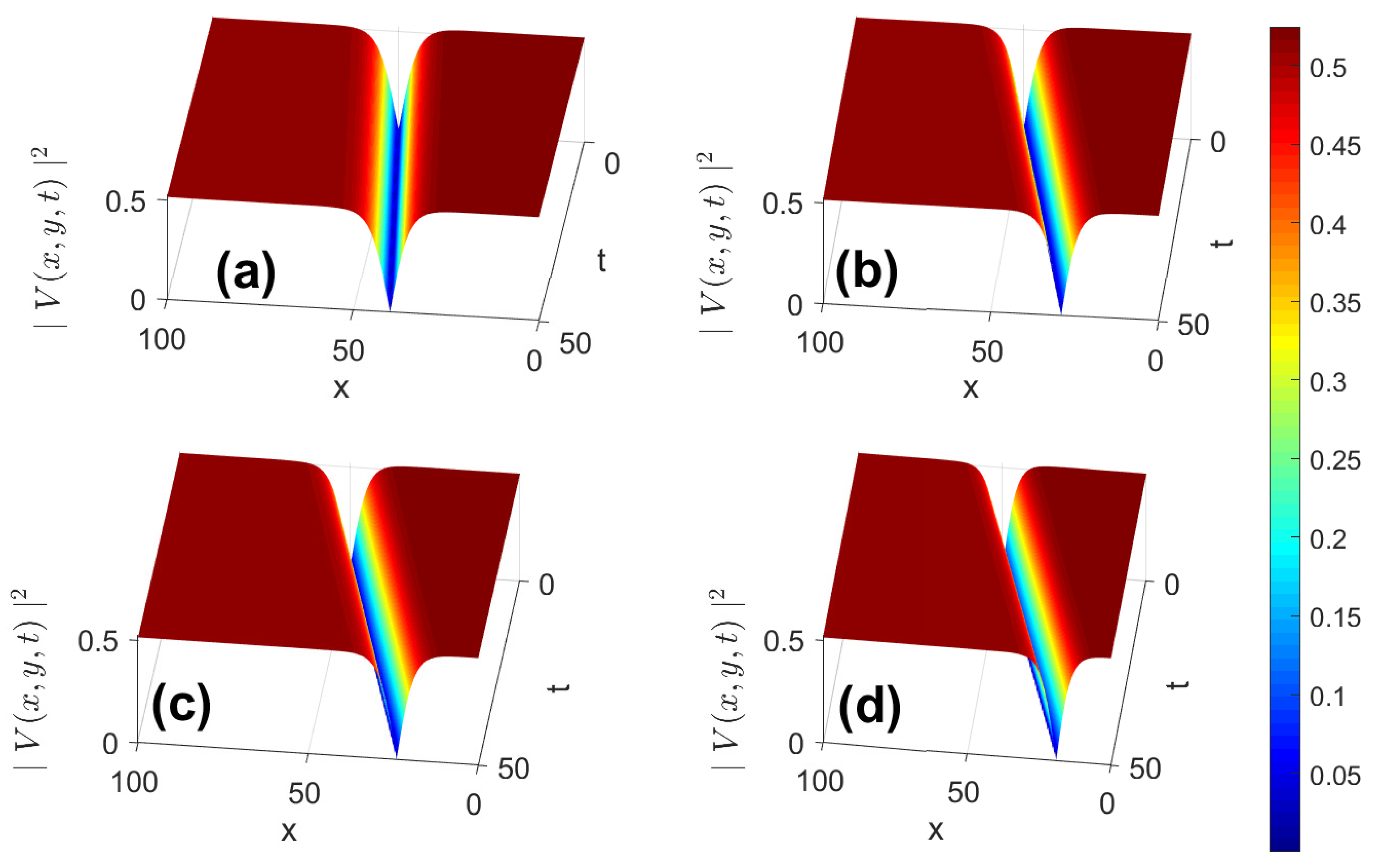
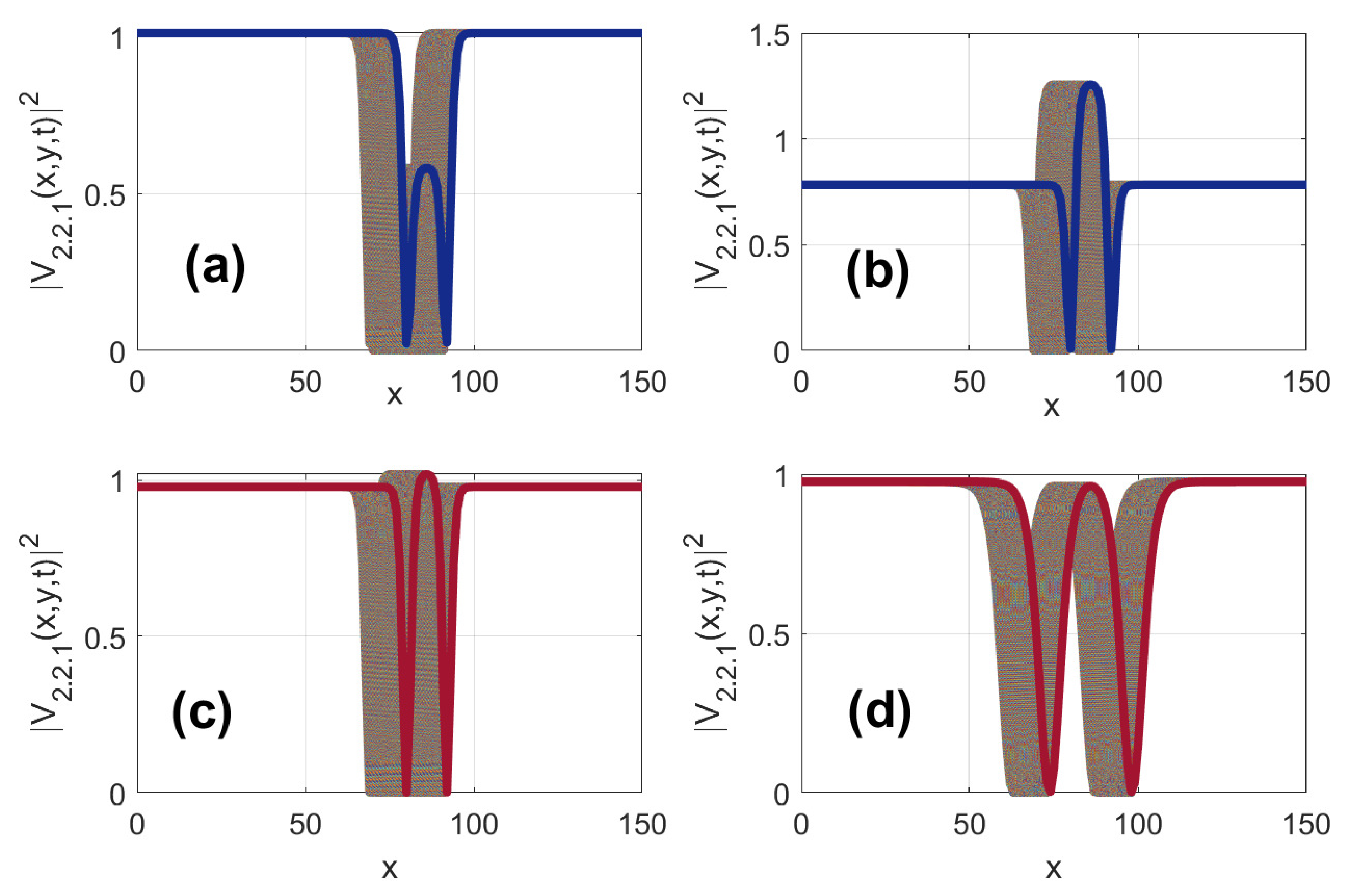
• Case 1: ${\lambda }_2>0,{\lambda }_4<0,$ and $p>0,q>0$, and a bright and singular soliton is obtained

$$\begin{array}{c}{\varphi }_1^{\pm }\left(\xi \right)=\pm \sqrt{-\frac{pq{\lambda }_2}{{\lambda }_4}}sec{h}_{pq}\left(\sqrt{{\lambda }_2}\xi \right),\end{array}$$

(19)

and

$$\begin{array}{c}{\varphi }_2^{\pm }\left(\xi \right)=\pm \sqrt{\frac{pq{\lambda }_2}{{\lambda }_4}}csc{h}_{pq}\left(\sqrt{{\lambda }_2}\xi \right).\end{array}$$

(20)

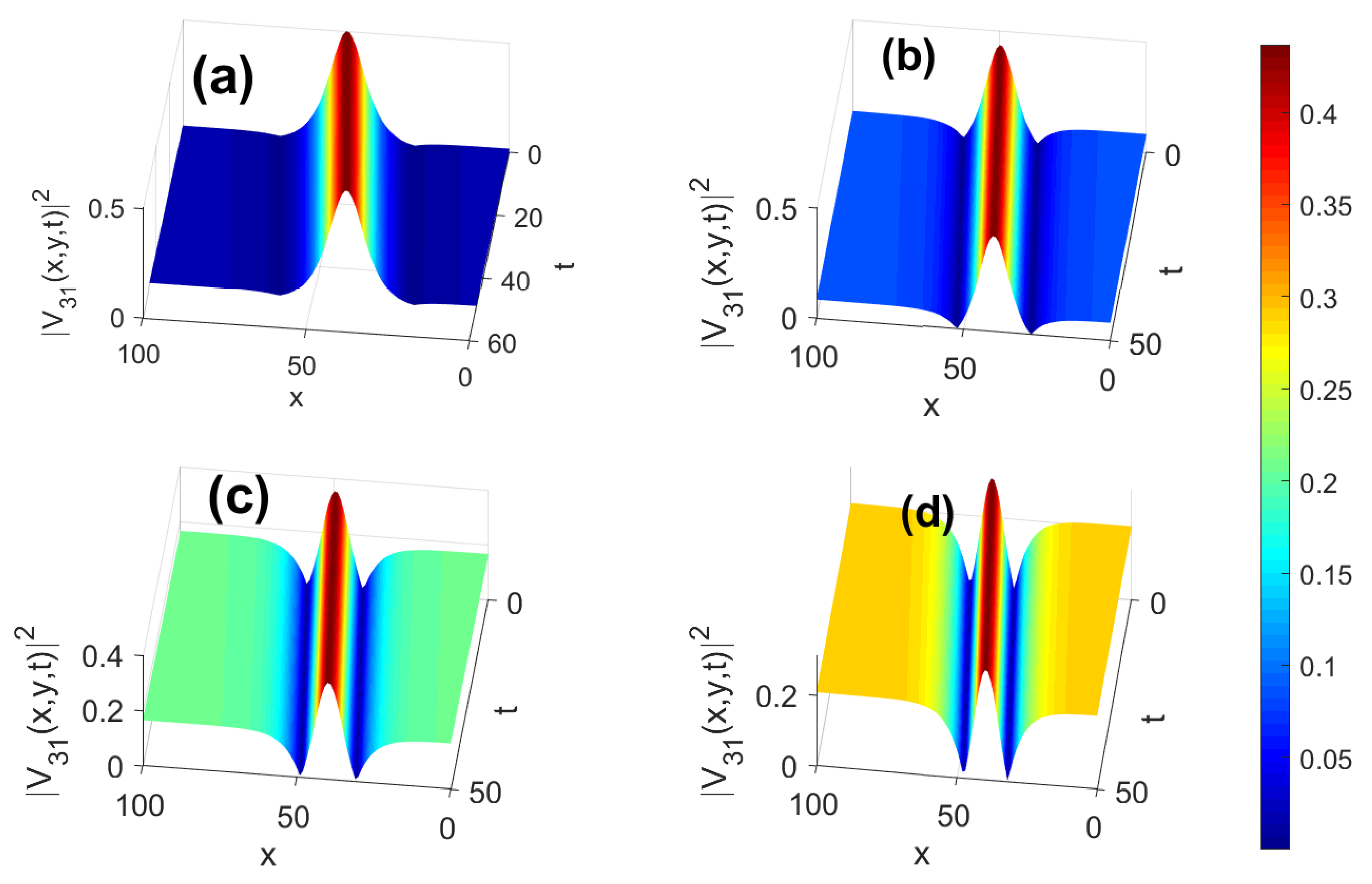
• Case 2: ${\lambda }_2<0,{\lambda }_4>0,$ and ${\lambda }_4\ne 0,$$p>0,q>0$, and we obtained periodic and singular solutions

  $$\begin{array}{c}{\varphi }_3^{\pm }\left(\xi \right)=\pm \sqrt{-\frac{pq{\lambda }_2}{{\lambda }_4}}{\sec }_{pq}\left(\sqrt{-{\lambda }_2}\xi \right),\end{array}$$

  (21)

  and

  $$\begin{array}{c}{\varphi }_4^{\pm }\left(\xi \right)=\pm \sqrt{-\frac{pq{\lambda }_2}{{\lambda }_4}}{\csc }_{pq}\left(\sqrt{-{\lambda }_2}\xi \right).\end{array}$$

  (22)

To examine the behavior of the NETL on the solitonic waves, we insert Equation (19) into Equation (18) and use Equation (17). We obtain

$$\begin{array}{c}{V}_{\mathrm{2.2.1}}\left(\xi \right)=B_0+\frac{3B_0\left(-2\beta B_0+\alpha \right)\left(1-{\left({\varphi }_1\left(\xi \right)\right)}^2\right)}{\alpha \left(1+{\left({\varphi }_1\left(\xi \right)\right)}^2\right)}.\end{array}$$

(23)

For ${\lambda }_0=\frac{1}{4}\frac{{\lambda }_2^2}{{\lambda }_4}$ it is obtained

• Result 3:

$$\begin{array}{c}{B}_0=B_0,B_1=B_1=2\sqrt{\frac{B_0\left(-3\beta B_0+2\alpha \right)}{3\beta }},\\ B_2=\sqrt{-\frac{3B_0\left(-3\beta B_0+2\alpha \right)}{3\beta }},{\lambda }_2=-\frac{{8748\alpha }^2{\beta }^3{\left(u_0^2+w_0^2\right)}^3}{{\vartheta }_0^{6}k{\left(2{\alpha }^2-9\beta \right)}^4},\\ {\lambda }_4=\frac{{1458\beta }^4{\left(u_0^2+w_0^2\right)}^3\left(18\sqrt{3}{B}_2{B}_0^2{\beta }^2-54B_0^3{\beta }^2-12\sqrt{3}{B}_2{B}_0\alpha \beta +54B_0^2\alpha \beta +\sqrt{3}{B}_2{\alpha }^2-12B_0{\alpha }^2\right)}{{B_2}^6{B}_0\left(-3\beta B_0+2\alpha \right)k^2{\left(2{\alpha }^2-9\beta \right)}^4},\\ \delta =-\frac{{{\vartheta }_0}^2\left(2{\alpha }^2-9\beta \right)}{9\beta \left(u_0^2+w_0^2\right)},k=k,\end{array}$$

(24)

with the constraint condition $\left(-3\beta B_0+2\alpha \right)k^2{\left(2{\alpha }^2-9\beta \right)}^4\ne 0.$

Thus, the general form of the solution gives

$$\begin{array}{c}V\left(\xi \right)=B_0+\frac{B_1{\varphi }_{\ell }\left(\xi \right)}{1+{\varphi }_{\ell }^2\left(\xi \right)}+\frac{B_2(1-{\varphi }_{\ell }^2\left(\xi \right))}{1+{\varphi }_{\ell }^2\left(\xi \right)},\ell =5,\dots ,14.\end{array}$$

(25)

Consequently,

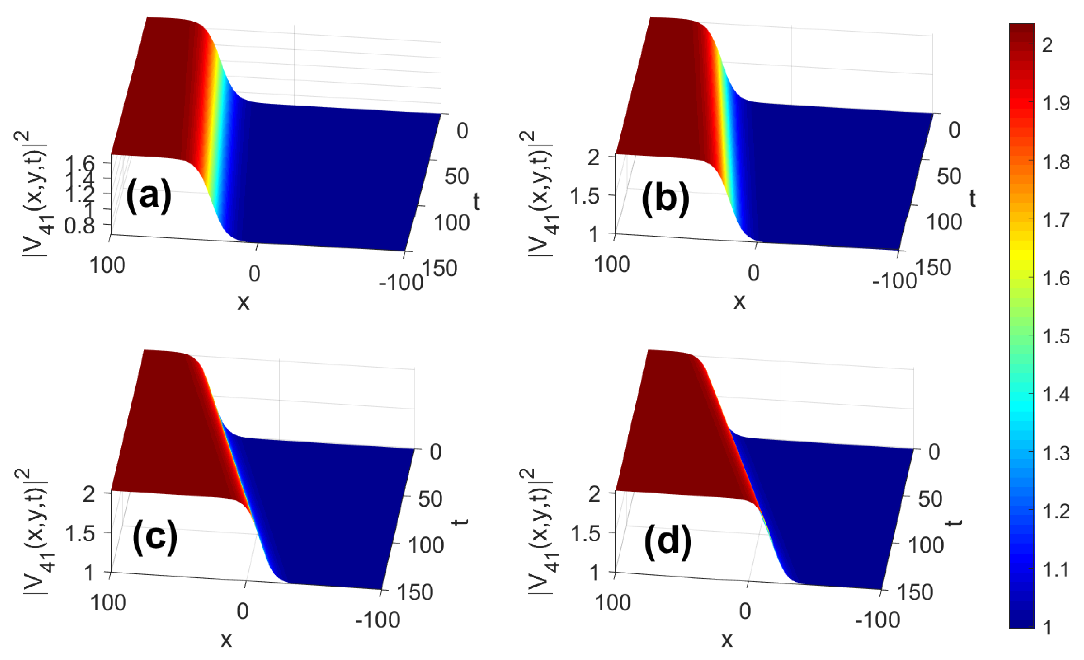
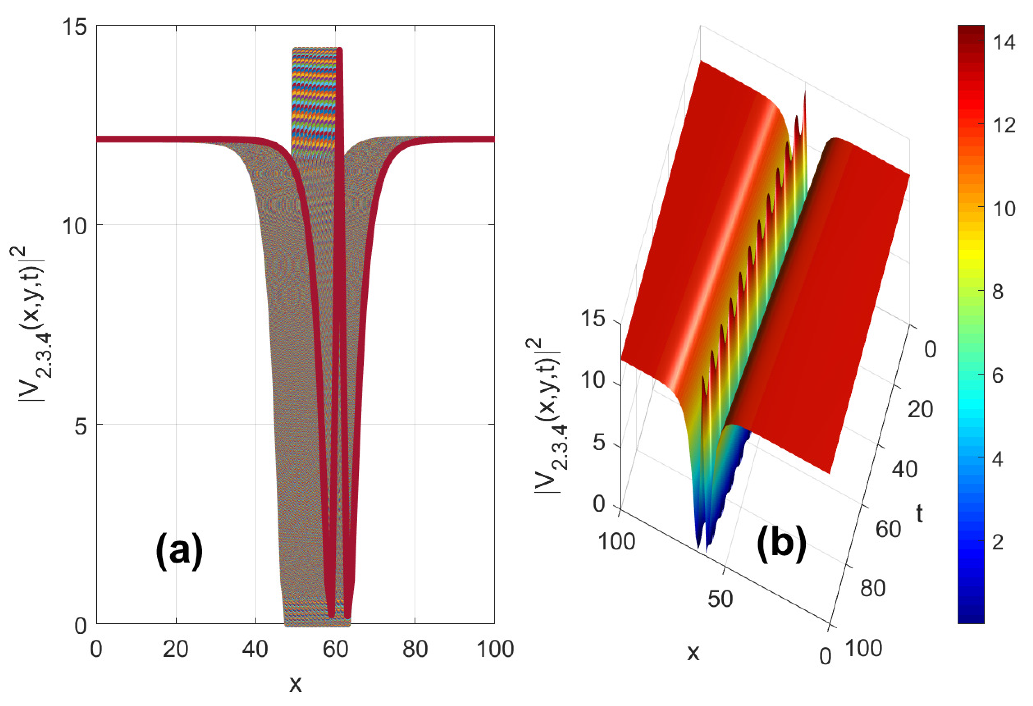
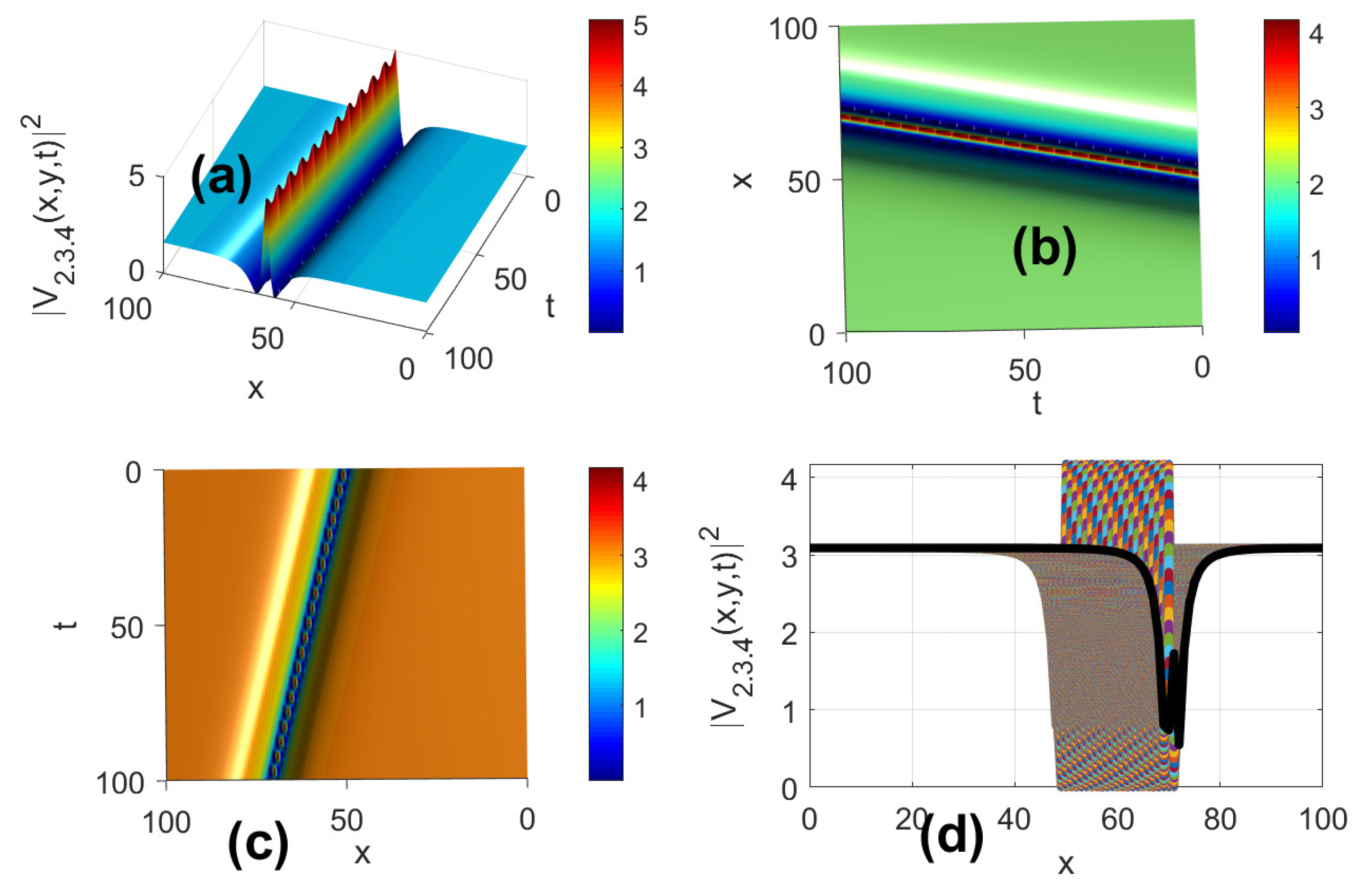
• Case 4: If ${\lambda }_2>0,{\lambda }_4<0,$ and we obtain trigonometric function solutions in the form

$$\begin{array}{c}{\varphi }_5^{\pm }\left(\xi \right)=\pm \frac{1}{2}\sqrt{\frac{2{\lambda }_2}{{\lambda }_4}}{\tan }_{pq}\left(\frac{1}{2}\sqrt{2{\lambda }_2}\xi \right),\end{array}$$

(26)

$$\begin{array}{c}{\varphi }_6^{\pm }\left(\xi \right)=\pm \frac{1}{2}\sqrt{\frac{2{\lambda }_2}{{\lambda }_4}}{\cot }_{pq}\left(\frac{1}{2}\sqrt{2{\lambda }_2}\xi \right),\end{array}$$

(27)

$$\begin{array}{c}{\varphi }_7^{\pm }\left(\xi \right)=\pm \frac{1}{2}\sqrt{\frac{2{\lambda }_2}{{\lambda }_4}}\left({\tan }_{pq}\right(\sqrt{2{\lambda }_2}\xi )\pm \sqrt{pq}{\sec }_{pq}(\sqrt{2{\lambda }_2}\xi \left)\right),\end{array}$$

(28)

$$\begin{array}{c}{\varphi }_8^{\pm }\left(\xi \right)=\pm \frac{1}{2}\sqrt{\frac{2{\lambda }_2}{{\lambda }_4}}\left({\cot }_{pq}\right(\sqrt{2{\lambda }_2}\xi )\pm \sqrt{pq}{\csc }_{pq}(\sqrt{2{\lambda }_2}\xi \left)\right),\end{array}$$

(29)

$$\begin{array}{c}{\varphi }_9^{\pm }\left(\xi \right)=\pm \frac{1}{4}\sqrt{\frac{2{\lambda }_2}{{\lambda }_4}}\left({\tan }_{pq}\left(\sqrt{\frac{{\lambda }_2}{8}}\xi \right)\pm \sqrt{pq}{\cot }_{pq}\left(\sqrt{\frac{{\lambda }_2}{8}}\xi \right)\right),\end{array}$$

(30)

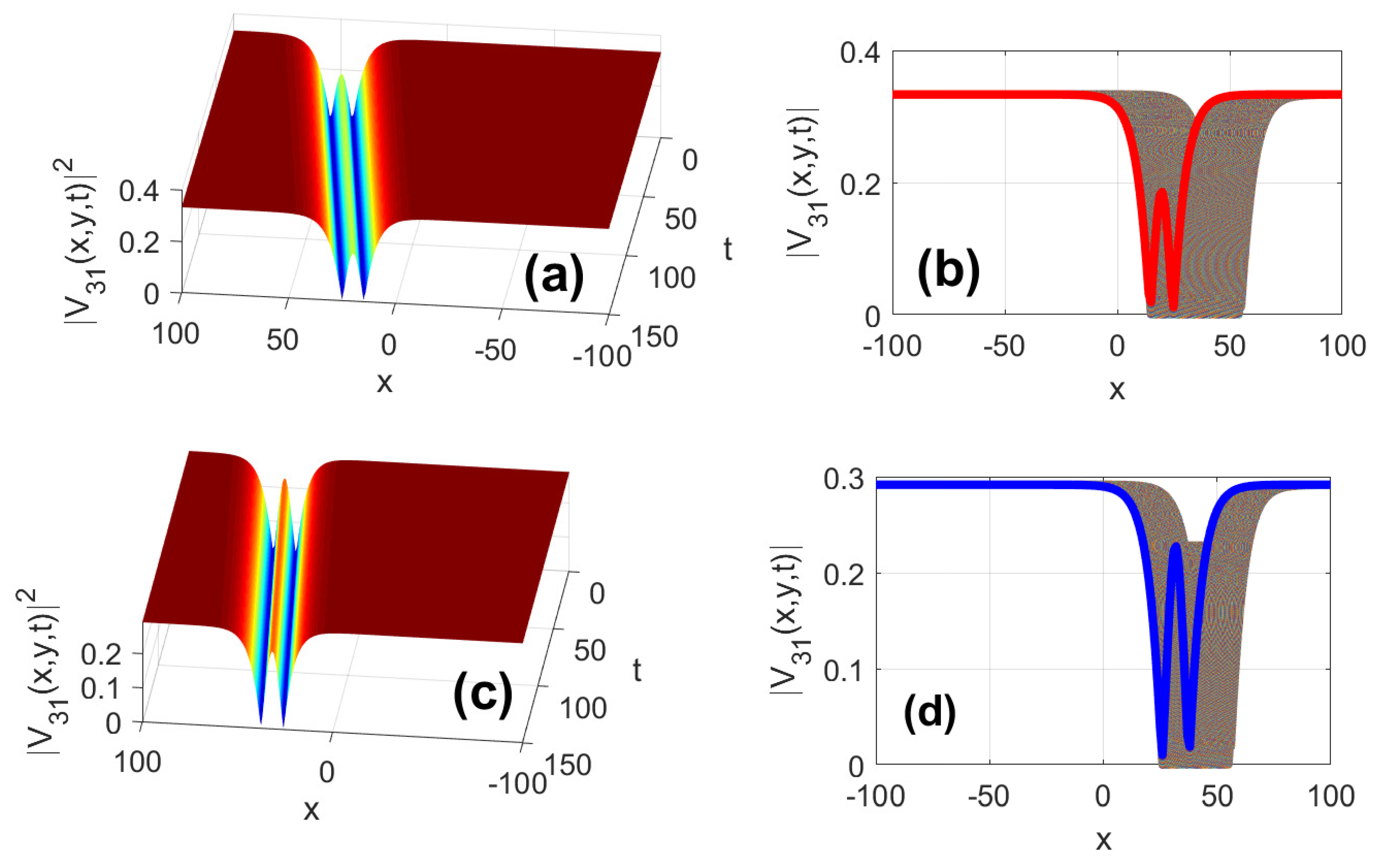
• Case 5: If ${\lambda }_2<0,{\lambda }_4>0,$ we obtain dark, singular and combined soliton solutions in the structure as

$$\begin{array}{c}{\varphi }_{10}^{\pm }\left(\xi \right)=\pm \frac{1}{2}\sqrt{-\frac{2{\lambda }_2}{{\lambda }_4}}{\tanh }_{pq}\left(\frac{1}{2}\sqrt{-2{\lambda }_2}\xi \right),\end{array}$$

(31)

$$\begin{array}{c}{\varphi }_{11}^{\pm }\left(\xi \right)=\pm \frac{1}{2}\sqrt{-\frac{2{\lambda }_2}{{\lambda }_4}}{\coth }_{pq}\left(\frac{1}{2}\sqrt{-2{\lambda }_2}\xi \right),\end{array}$$

(32)

$$\begin{array}{c}{\varphi }_{12}^{\pm }\left(\xi \right)=\pm \frac{1}{2}\sqrt{-\frac{2{\lambda }_2}{{\lambda }_4}}\left({\tanh }_{pq}\right(\sqrt{-2{\lambda }_2}\xi )\pm i\sqrt{pq}sec{h}_{pq}(\sqrt{-2{\lambda }_2}\xi \left)\right),\end{array}$$

(33)

$$\begin{array}{c}{\varphi }_{13}^{\pm }\left(\xi \right)=\pm \frac{1}{2}\sqrt{-\frac{2{\lambda }_2}{{\lambda }_4}}\left({\coth }_{pq}\right(\sqrt{-2{\lambda }_2}\xi )\pm \sqrt{pq}csc{h}_{pq}(\sqrt{-2{\lambda }_2}\xi \left)\right),\end{array}$$

(34)

$$\begin{array}{c}{\varphi }_{14}^{\pm }\left(\xi \right)=\pm \frac{1}{4}\sqrt{-\frac{2{\lambda }_2}{{\lambda }_4}}\left({\tanh }_{pq}\left(\sqrt{\frac{-{\lambda }_2}{8}}\xi \right)\pm \sqrt{pq}{\coth }_{pq}\left(\sqrt{\frac{-{\lambda }_2}{8}}\xi \right)\right),\end{array}$$

(35)

with p and q constants greater than zero, which are called deformation parameters.

$\begin{array}{c}sec{h}_{pq}\left(\xi \right)=\frac{2}{p{e}^{\xi }+q{e}^{-\xi }} , csc{h}_{pq}\left(\xi \right)=\frac{2}{p{e}^{\xi }-q{e}^{-\xi }} , se{c}_{pq}\left(\xi \right)=\frac{2}{p{e}^{i\xi }+q{e}^{-i\xi }},\hfill \\ cs{c}_{pq}\left(\xi \right)=\frac{2i}{p{e}^{i\xi }-q{e}^{-i\xi }} , {\tanh }_{pq}\left(\xi \right)=\frac{p{e}^{\xi }-q{e}^{-\xi }}{p{e}^{\xi }+q{e}^{-\xi }} , {\coth }_{pq}\left(\xi \right)=\frac{p{e}^{\xi }+q{e}^{-\xi }}{p{e}^{\xi }-q{e}^{-\xi }},\hfill \\ {\tan }_{pq}\left(\xi \right)=-i\frac{p{e}^{i\xi }-q{e}^{-i\xi }}{p{e}^{i\xi }+q{e}^{-i\xi }} \mathrm{and} {\cot }_{pq}\left(\xi \right)=i\frac{p{e}^{i\xi }+q{e}^{-i\xi }}{p{e}^{i\xi }-q{e}^{-i\xi }}.\hfill \end{array}$

In Figure 5a,b, we display the spatiotemporal evolution of the W-SS with variation in the potential parameters. From Figure 5a, we keep the parameter $\beta =0.012V^{-1}$ fixed and set $\alpha =0.19V^{-1}$ and $\alpha =0.29V^{-1}$, respectively. We show that its amplitude increases to $1.5$. Additionally, we fix the potential parameter $\alpha =0.2V^{-1}$ and increase the value of the potential parameter $\beta =0.019V^{-1}$, which shows that the W-formed has increased to reach 1. By increasing the value of the potential parameter $\beta =0.02V^{-1}$, the W-shaped is well formed and maintains its fixed amplitude, as shown in Figure 5d.

Now, we insert Equation (31) into Equation (25) with Equation (24) and the following is obtained:

$$\begin{array}{c}{V}_{\mathrm{2.3.4}}\left(\xi \right)=B_0+\frac{B_1{\varphi }_5\left(\xi \right)}{1+{\varphi }_5^2\left(\xi \right)}+\frac{B_2(1-{\varphi }_5^2\left(\xi \right))}{1+{\varphi }_5^2\left(\xi \right)}.\end{array}$$

(36)

In Figure 6a,b, we show the evolution of the W-SS for suitable parameters of the NELT. It is shown that, for ${\lambda }_2<0$ and ${\lambda }_4>0$, the W-shaped emerges in the structure with a higher amplitude than in the case of ${\lambda }_2>0$ and ${\lambda }_4<0$. With the same conditions, in Figure 7a–d, we show the W-shaped profile with the effects of the NELT parameters. One can observe that the potential parameters and the parameters of the auxiliary equation are all important in the system and they are behaving as sources of energy.

4. Conclusions

In this work, we used the JEF and auxiliary equation methods to construct the exact traveling waves soliton propagating along a nonlinear electrical transmission line. We used the transformation hypothesis to acquire the NODE. It is assumed that ${\lambda }_1=0$ and ${\lambda }_3=0$ lead to a family of Jacobi elliptic function solutions being obtained. Thereafter, we apply a new form of the general solution to point out bright, dark, W-shaped soliton, combined trigonometric solutions and combined complex solutions, and a singular soliton also emerges under certain conditions on the auxiliary equation parameters. One can observe that the outcomes of this work cover a wide class of soliton solutions. Without a doubt, these solutions will be helpful for solitary wave theory and data transport in telecommunication systems.

References

- Sekulic, D.L.; Satoric, M.V.; Zivanov, M.B.; Bajic, J.S. Soliton-like pulses along electrical nonlinear transmission line. Elecron. Electr. Eng. 2012, 121, 53. [Google Scholar] [CrossRef] [Green Version]
- Pelap, F.B.; Faye, M. Soliton-like excitations in the one-dimensional electrical transmission line. Nonlinear Oscil. 2005, 8, 513–525. [Google Scholar] [CrossRef]
- Marquié, P.; Bibault, J.M.; Remoissenet, M. Generation of envelope and hole solitons in an experimental transmission line. Phys. Rev. E 1995, 51, 6127. [Google Scholar] [CrossRef] [PubMed]
- Kenmogne, F.; Yemélxex, D. Bright and peaklike pulse solitary waves and analogy with modulational instability in an extended nonlinear Schrödinger equation. Phys. Rev. E 2013, 88, 207. [Google Scholar] [CrossRef] [PubMed]
- Peterson, G.E. Electrical transmission lines as models for soliton propagation in materials: Elementary aspects of video solitons. AT Bell Lab. Tech. J. 1984, 63, 901. [Google Scholar] [CrossRef]
- Yazaki, T.; Fukushima, K. Experimental studies of potential problems in quantum mechan-ics using nonlinear transmission line. Am. J. Phys. 1985, 53, 1186. [Google Scholar] [CrossRef]
- Nejoh, Y. Envelope soliton of the electron plasma wave in a nonlinear transmission line. Phys. Scr. 1985, 31, 415. [Google Scholar] [CrossRef]
- Paulus, P.; Wedding, B.; Gasch, A.; Jager, D. Bistability and solitons observed in a nonlinear ring resonator. Phys. Lett. A 1984, 102A, 89. [Google Scholar] [CrossRef]
- Hirota, R.; Suzuki, K. Theoretical and experimental studies of lattice solitons in nonlinear lumped networks. Proc. IEEE 1973, 13, 1483–1491. [Google Scholar] [CrossRef]
- Hirota, R.; Suzuki, K. Field Distribution in a Magnetoplasma-Loaded Waveguide at Room Temperature. Trans. IEEE 1970, 18, 915–916. [Google Scholar] [CrossRef]
- Freeman, R.H.; Karbowiak, A.E. An investigation of nonlinear transmission lines and shock waves. J. Phys. D Appl. Phys. 1977, 10, 633. [Google Scholar] [CrossRef]
- Watanabe, S. Soliton and generation of tail in nonlinear dispersive media with weak dissi-pation. J. Phys. Soc. Jpn. 1978, 45, 276. [Google Scholar] [CrossRef]
- Yoshinaga, T.; Kakutani, T. Second order KDV soliton on a nonlinear transmission line. J. Phys. Soc. Jpn. 1980, 49, 2072. [Google Scholar] [CrossRef]
- Nogushi, A. Solitons in a Nonlinear Inhomogeneous Transmission Line. Electron. Commun. Jpn. 1974, 57, 9. [Google Scholar]
- Jager, D.; Tegude, F.J. Nonlinear wave propagation along periodic-loaded transmission line. Appl. Phys. 1978, 15, 393. [Google Scholar] [CrossRef]
- Fukushima, K.; Wadati, M.; Kotera, T.; Sawada, K.; Narahara, Y. Experimental and theo-retical study of the recurrence phenomena in nonlinear transmission line. J. Phys. Soc. Jpn. 1980, 48, 1029. [Google Scholar] [CrossRef]
- Nagashina, H.; Amagishi, Y. Experiment on Solitons in the Dissipative Toda Lattice Using Nonlinear Transmission Line. J. Phys. Soc. Jpn. 1978, 45, 680. [Google Scholar] [CrossRef]
- Kofané, T.C.; Michaux, B.; Remoissenet, M. Theoretical and experimental studies of diatomic lattice solitons using an electrical transmission line. J. Phys. C Solid Stat. Phys. 1988, 21, 1395. [Google Scholar] [CrossRef]
- Benson, F.A.; Last, J.D. Nonlinear Transmission Line Harmonic Generator. Proc. IEEE 1965, 112, 635. [Google Scholar] [CrossRef]
- Yagi, T.; Noguchi, A. Gyromagnetic nonlinear element and its application as a pulse-shaping transmission line. Proc. Lett. 1977, 13, 683. [Google Scholar] [CrossRef]
- Tan, M.; Su, C.; Anklam, W. 7× electrical pulse compression an inhomogeneous nonlinear transmission line. Electron. Lett. 1988, 24, 213. [Google Scholar] [CrossRef]
- Abdoulkary, S.; Mohamadou, A.; Beda, T. Exact traveling discrete kink-soliton solutions for the discrete nonlinear electrical transmission lines. Commun. Nonlinear Sci. Numer. Simul. 2011, 16, 3525. [Google Scholar] [CrossRef]
- Kegne, E. Nonlinear wave transmission in a two-dimensional nonlinear electric transmis-sion network with dissipative elements. Chaos Solitons Fractals 2022, 164, 112637. [Google Scholar] [CrossRef]
- Djelah, G.; Ndzana, F.I.I.; Abdoulkary, S.; Mohamadou, A. First and second order rogue waves dynamics in a nonlinear electrical transmission line with the next nearest neighbor couplings. Chaos Solitons Fractals 2023, 167, 113087. [Google Scholar] [CrossRef]
- Zhang, L.-H. Travelling wave solutions for the generalized Zakharov-Kuznetsov equation with higher-order nonlinear terms. Appl. Math. Comput. 2009, 208, 144–155. [Google Scholar] [CrossRef]
- Fermi, E.; Pasta, J.; Ulam, S. Collected papers of Enrico Fermi II; University of Chicago Press: Chicago, IL, USA, 1965. [Google Scholar]
- Agrawal, G.P. Nonlinear Fiber Optics, 2nd ed.; Academic: New York, NY, USA, 1995. [Google Scholar]
- Hirota, R.; Suzuki, K. Studies on lattice solitons by using electrical networks. J. Phys. Soc. Jpn. 1970, 28, 1366. [Google Scholar] [CrossRef]
- Ren, Z.; Ying, C.; Fan, C.; Wu, Q. The Generation Mechanism of Airy-Bessel Wave Packets in Free Space. Chin. Phys. Lett. 2012, 29, 124209. [Google Scholar] [CrossRef]
- Zhong, W.P.; Belić, M.R.; Huang, T. Two-Dimensional accessible solitons in P T-symmetric potentials. Nonlinear Dyn. 2012, 70, 2027–2034. [Google Scholar] [CrossRef]
- Zhong, W.-P.; Belić, M.R. Soliton tunneling in the nonlinear Schrödinger equation with variable coefficients and an external harmonic potential. Phys. Rev. E 2010, 81, 056604. [Google Scholar] [CrossRef]
- Zhong, W.-P.; Belić, M.R.; Huang, T. Rogue wave solutions to the generalized nonline-ar Schrödinger equation with variable coefficients. Phys. Rev. E 2013, 87, 065201. [Google Scholar] [CrossRef]
- Zhong, W.-P.; Belić, M.R.; Huang, T. Three-dimensional finite-energy Airy self-accelerating parabolic-cylinder light bullets. Phys. Rev. A 2013, 88, 033824. [Google Scholar] [CrossRef]
- Zhong, W.-P.; Belić, M.R.; Zhang, M.B.A.Y.; Huang, T. Spatiotemporal accessible sol-itons in fractional dimensions. Phys. Rev. E 2016, 94, 012216. [Google Scholar] [CrossRef] [PubMed] [Green Version]
- Yang, Z.; Zhong, W.-P.; Belić, M.; Zhang, Y. Controllable optical rogue waves via non-linearity management. Opt. Express 2018, 26, 7587. [Google Scholar] [CrossRef]
- Hirota, R. Exact solution of the Korteweg-de-Vries equation for multiple collisions of soli-tons. Phys. Rev. Lett. 1971, 27, 1192–1194. [Google Scholar] [CrossRef]
- Tsigaridas, G.; Fragos, A.; Polyzos, I.; Fakis, M.; Ioannou, A.; Gianneta, V.; Persophonis, P. Evolution of near-soliton initial profiles in nonlinear wave equations through their Backlund transforms. Chaos Solitons Fractals 2005, 23, 1841–1854. [Google Scholar] [CrossRef]
- Suzo, A.A. Intertwining technique for the matrix Schrödinger equation. Phys. Lett. A 2005, 335, 88–102. [Google Scholar] [CrossRef]
- Banerjee, R.S. Painleve´ analysis of the K(m,n) equations which yield compac-tons. Phys. Scr. 1998, 57, 598–600. [Google Scholar] [CrossRef]
- Yan, Z.Y.; Zhang, H.Q. New explicit solitary wave solutions and periodic wave solutions for Whitham-Broer-Kaup equation in shallow water. Phys. Lett. A 2001, 285, 355–362. [Google Scholar] [CrossRef]
- He, J.H. The variational iteration method for eighth-order initial-boundary value problems. Phys. Scr. 2007, 76, 680–682. [Google Scholar] [CrossRef]
- Dai, C.Q.; Wang, Y.-Y. Exact travelling wave solutions of the discrete nonlinear Schrödinger equation and the hybrid lattice equation obtained via the exp-function method. Phys. Scr. 2008, 78, 015013–015019. [Google Scholar] [CrossRef]
- Hu, J. An algebraic method exactly solving two high-dimensional nonlinear evolution equa-tions. Chaos Solitons Fractals 2005, 23, 391–398. [Google Scholar]
- Dursun, I.; Idris, D. Solitary wave solutions of the CMKDV equation by using the quintic B-spline collocation method. Phys. Scr. 2008, 77, 065001–065008. [Google Scholar]
- Kudryashov, N.A. One method for finding exact solutions of nonlinear differential equations. Commun. Nonlinear Sci. Numer. Simul. 2012, 17, 2248–2253. [Google Scholar] [CrossRef] [Green Version]
- Ryabov, P.N.; Sinelshchikov, D.I.; Kochanov, M.B. Exact solutions of the Kudryash-ov-Sinelshchikov equation using the multiple (G′G)-expansion method. Appl. Math. Comput. 2011, 218, 3965–3972. [Google Scholar]
- Malwe, B.H.; Gambo, B.; Doka, S.Y.; Kofane, T.C. Soliton wave solutions for the nonlin-ear transmission line using Kudryashov method and (G′/G)-expansion method. Appl. Math. Comput. 2014, 239, 299–309. [Google Scholar]
- Kudryashov, N.A. Simplest equation method to look for exact solutions of nonlinear differ-ential equation. Chaos Solitons Fractals 2005, 24, 1217–1221. [Google Scholar] [CrossRef] [Green Version]
- Lu, D.; Seadawy, A.R.; Arshad, M.; Wang, J. New solitary wave solutions of (3 + 1)-dimensional nonlinear extended Zakharov-Kuznetsov and modified KdV-Zakharov-Kuznetsov equa-tions and their applications. Results Phys. 2017, 7, 899–909. [Google Scholar] [CrossRef]
- Arshad, M.; Seadawy, A.R.; Lu, D.; Wang, J. Travelling wave solutions of generalized cou-pled Zakharov-Kuznetsov and dispersive long wave equations. Results Phys. 2016, 6, 1136–1145. [Google Scholar] [CrossRef] [Green Version]
- Tala-Tebue, E.; Tsobgni-Fozap, D.C.; Kenfack-Jiotsa, A.; Kofane, T.C. Envelope periodic solutions for a discrete network with the Jacobi elliptic functions and the alternative (G′/G)-expansion method including the generalized Riccati equation. Eur. Phys. J. Plus 2009, 129, 136–146. [Google Scholar] [CrossRef]
- Gladkov, S.O.; Aung, Z. Regarding corrections to the Stokes force in the Knudsen number. Russ. Phys. J. 2021, 63, 2122–2140. [Google Scholar] [CrossRef]
- Fairbanks, A.J.; Darr, A.M.; Garner, A.L. A review of nonlinear transmission line system design. IEEE Access 2020, 8, 148606–148621. [Google Scholar] [CrossRef]
- Crawford, T.D.; Garner, A.L. Nonlinear Transmission Line Performance as a Combined Pulse Forming Line and High-Power Microwave Source as a Function of Line Impedance. Appl. Sci. 2022, 12, 10305. [Google Scholar] [CrossRef]
Disclaimer/Publisher’s Note: The statements, opinions and data contained in all publications are solely those of the individual author(s) and contributor(s) and not of MDPI and/or the editor(s). MDPI and/or the editor(s) disclaim responsibility for any injury to people or property resulting from any ideas, methods, instructions or products referred to in the content. |
© 2023 by the authors. Licensee MDPI, Basel, Switzerland. This article is an open access article distributed under the terms and conditions of the Creative Commons Attribution (CC BY) license (https://creativecommons.org/licenses/by/4.0/).
Share and Cite
Inc, M.; Alqahtani, R.T.; Agarwal, R.P. W-Shaped Bright Soliton of the (2 + 1)-Dimension Nonlinear Electrical Transmission Line. Mathematics 2023, 11, 1703. https://doi.org/10.3390/math11071703
Inc M, Alqahtani RT, Agarwal RP. W-Shaped Bright Soliton of the (2 + 1)-Dimension Nonlinear Electrical Transmission Line. Mathematics. 2023; 11(7):1703. https://doi.org/10.3390/math11071703
Chicago/Turabian StyleInc, Mustafa, Rubayyi T. Alqahtani, and Ravi P. Agarwal. 2023. "W-Shaped Bright Soliton of the (2 + 1)-Dimension Nonlinear Electrical Transmission Line" Mathematics 11, no. 7: 1703. https://doi.org/10.3390/math11071703