A Generalized Mathematical Model of Toxoplasmosis with an Intermediate Host and the Definitive Cat Host

Abstract

In this paper, we construct a generalized epidemiological mathematical model to study toxoplasmosis dynamics, taking into consideration both cat and mouse populations. The model incorporates generalized proportions for the congenital transmission in the mouse and cat populations, along with the oocysts available in the environment. We focus on determining the conditions under which toxoplasmosis can be eradicated. We conduct a stability analysis in order to reveal the dynamics of toxoplasmosis in the cat and mouse populations; moreover, we compute the basic reproduction number ${\mathcal{R}}_0$, which is crucial for the long-term behavior of the toxoplasmosis disease in these populations as well as the steady states related to both populations. We find that vertical transmission in the cat population is essential, and affects the basic reproduction number ${\mathcal{R}}_0$. If full vertical transmission is considered in the mouse population and ${\mathcal{R}}_0<1$, we find that all solutions converge to the limit set comprised by the infinitely many toxoplasmosis-free-cat steady states, meaning that toxoplasmosis would vanish from the cat population regardless of the initial conditions. On the other hand, if ${\mathcal{R}}_0>1$, then there is only one toxoplasmosis-endemic steady state. When full vertical transmission is not considered in the mouse population, then a unique toxoplasmosis-free equilibrium exists and toxoplasmosis can be eradicated for both the cat and mouse populations. This has important public health implications. Numerical simulations are carried out to reinforce our theoretical stability analysis and observe the repercussion of some parameters on the dynamics.

1. Introduction

Toxoplasma gondii is a parasite that is common in a variety of animals. Cats are the main hosts, and the parasite is transmitted by various paths [1,2,3]. In cats, the parasite completes its whole life cycle without impacting their life. Cats can eject more than 20 million oocysts [4]. In preganant cats, T. gondii can be transmitted to the fetus [5]. It is important to point out that cats are among the most popular pets in the world [6].

More than 40 million people in the U.S. carry the Toxoplasma parasite. However, most of these people do not have infections due to the protection provided by their immune systems [7,8]. T. gondii is a parasite that is able to infect many species of warm-blooded animals, including humans [7,8]. T. gondii infection is very common in different parts of the world. It has been reported that its seroprevalence in cats and humans can be around 30 to 40 percent [9]. The only known definitive hosts for T. gondii are members of the family Felidae, which includes domestic cats. A cat that is infected sheds oocysts in its feces; the oocysts can then contaminate the surroundings, including water and food [7,9,10,11]. Several types of meat are important sources of infections of Toxoplasma [12]. It has been reported that gamma irradiation can kill oocysts that are present in foods [11]. Oocysts are spread by different means, including water and wind Intermediate hosts can become infected by consuming oocysts present in the water or in the environment [7,8,13]. In addition, it has been reported that cats can shed oocysts after they have ingested infected mice [13]. Toxoplasma infection can be acquired by humans due to eating cysts that are present in raw/uncooked meat [8,14]. In addition, it has been shown that cats are a major reservoir of this infection [8,9,15,16,17].

The consequences of toxoplasmosis infection during pregnancy are complicated. In this instance, in approximately 30% of cases the fetus suffers a congenital infection, in which neurological or eye problems may occur. The severity of these problems depend on the gestational age. Preventive protocols can help to reduce the severity of infection [18]. The placenta plays a direct role in T. gondii transmission to the fetus In [19], the authors evaluated congenital transmission via experiments on mice. They were able to determine parasite load and study further vertical transmission. In addition, it has been found that T. gondii in pregnant mice can be transmitted through the placenta [18,20]. Due to the similarities of human and rodent placentas, it is common to use mice as an experimental model of congenital toxoplasmosis [21,22]. Congenital transmission in mice has been noted in several consecutive generations [23]. Moreover, it has been suggested that previous infection with a particular T. gondii strain does not prevent toxoplasmosis in mice in the case of re-infection with another T. gondii strain [22,24]. Thus, the available evidence indicates that congenital transmission is common in populations of mice [25]. It has been suggested that the deer mouse could be a factor in maintaining T. gondii due to vertical transmission, despite the lack of feline hosts [23]. Finally, in [26], it was reported that transmission happens in at least 1% of fetal cases. The observed high percentages of vertical transmission in populations of mice, as well as in other populations, suggest that these transmissions are common.

It is possible that mice can help to maintain the propagation of T. gondii. In Manchester, UK, it was found that 59% of 200 mice taken from infested properties tested positive for Toxoplasma. It has been shown that vertical transmission from the infected dam to the fetus can occur, which could be another factor in maintaining infection rates in non-rural areas. It is important to take into account these results for the purposes of rodent control [27]; thus, in the present research we include congenital transmission in the mouse population in our mathematical model.

Mathematical models have been implemented to investigate epidemics involving parasites, viruses, and, recently, the COVID-19 pandemic [28,29,30,31]. While mathematical models in many fields are simplifications of the real world, they can nonetheless provide important insights into a wide variety of real processes. Mathematical modeling has been used broadly to investigate the dynamics of numerous diseases in various populations [28,31]. The dynamics of T. gondii infection have been explored using mathematical models with different approaches [17]. One approach is to focus the models on cat–human transmission [32,33]. These models vary depending on assumptions/hypotheses related to demographic factors and to horizontal and vertical transmission. More complex models include the transmission of T. gondii between susceptible and infected hosts at the population level [16,34,35]. In addition, articles have explored and incorporated the vaccination of cats and swine [16,34,35,36,37]. The involvement of vaccines in these models allows the outcomes of particular control strategies to be explored [38]. Vaccines can have a variety of effects. If vaccination is included in the model, it is assumed that it provides lifelong immunity [39,40]. Vaccines for cats are justified, as the T. gondii parasite has supportive circumstances for survival, especially in cats [15]. In addition, several researchers have proposed within-host models to study the dynamics of T. gondii invasion [41]. Recently, researchers have explored the effect of discrete time delay to see how this affects the dynamics of toxoplasmosis disease in the cat population [42,43]. For a detailed review of mathematical models related to toxoplasmosis, interested readers may refer to [17].

In this work, we design a generalized mathematical model to research toxoplasmosis dynamics in cat and mouse populations. The model incorporates congenital transmission in both the mouse and cat populations. The generalized model considers a much broader spectrum of possibilities than in our previous work, where partial congenital transmission was not considered [44]. In this study, the model includes infinitely many proportions of vertical transmissions for the mouse and cat populations. The model takes into account the possibility of transmission between oocysts and mice, and considers the option of vaccinating the cat population. In the model, cats can have three disease statuses, namely, infected, susceptible, and recovered/vaccinated, while mice can be either susceptible $S_m\left(t\right)$ or infected $I_m\left(t\right)$. In addition, the model encompasses T. gondii oocysts. We examine the stability of the equilibrium points of the system, and design suitable Lyapunov functions that let us demonstrate the global stability of the equilibrium points. Lyapunov functions have been used extensively to study the global stability of equilibrium points of epidemic models [45,46,47,48]. We compute the basic reproductive number ${\mathcal{R}}_0$ that is crucial for the dynamics of toxoplasmosis. We execute simulations in order to obtain useful insights into the dynamics of toxoplasmosis and to support our theoretical results; such simulations can additionally be used to explore the effect of public health strategies to control toxoplasmosis.

The rest of this manuscript is organized as follows. In Section 2 we design the toxoplasmosis mathematical model with intermediate and definitive hosts. Section 3 is devoted to the stability analysis of the equilibrium points and to computing the basic reproduction number ${\mathcal{R}}_0$. In addition, we build suitable Lyapunov functions that let us to demonstrate the global stability of the toxoplasmosis-free equilibrium point. Section 4 incorporates simulations of various scenarios, and finally in Section 5 conclusions are given.

2. Mathematical Model

Here, we modify and extend a mathematical model that has previously been used to examine the transmission of toxoplasmosis in cat populations [34]. A constant immunization program is included for the population of cats [16,34,35,36,37]. The model includes the oocyst population as a state variable due to oocysts being the primary reason for the persistence of T. gondii in the environment [9]. The cat is the only vector known to excrete T. gondii oocysts [7,9]. The proposed model contemplates encounters between the T. gondii oocysts adn both cats and mice. The model considers the probability of infection to be related to the amount of sporulated oocysts in the environment [36].

The generalized mathematical model is comprised of ordinary differential equations. Among the parameters of the model are those describing the birth, death, and vaccination rates. Other parameters are related to the lifespan of oocysts and their production by each infected cat. After infection or vaccination, it is assumed that cats have lifelong immunity [8]. A generalized proportion of vertical transmission is assumed in the definitive and intermediate hosts [23,24,49]. The model assumes that sporulated oocysts decay exponentially [17,34,35].

The developed model includes the following assumptions/hypotheses:

• Cats can be susceptible (S), infected (I), or recovered/vaccinated ($V_R$).
• The mouse population $N_m$ is divided into two classes, namely, susceptible ($S_m$) and infectious ($I_m$).
• Oocysts (O) denotes the amount of T. gondii oocysts.
• The mouse and cat populations are assumed to be constant.
• A susceptible mouse or cat moves to the infectious class after contact with T. gondii oocysts (at rates ${\beta }_m$ and $\beta$, respectively).
• A susceptible cat flows to the recovered/vaccinated class $V_R$ at a rate $\gamma$. An infectious cat flows to the vaccinated/recovered subpopulation $V_R\left(t\right)$ at a rate $\alpha$.
• T. gondii oocysts $O\left(t\right)$ are generated by infectious cats $I\left(t\right)$.
• ${\mu }_0$ is the degradation/removal rate of T. gondii oocysts in the environment.
• $\mu$ represents the birth and death rate for cats.
• ${\mu }_c$ represents the birth and death rate of mice.
• A proportion q of vertical transmittal is assumed in the cat population.
• A proportion p of vertical transmittal is assumed in the mouse population.

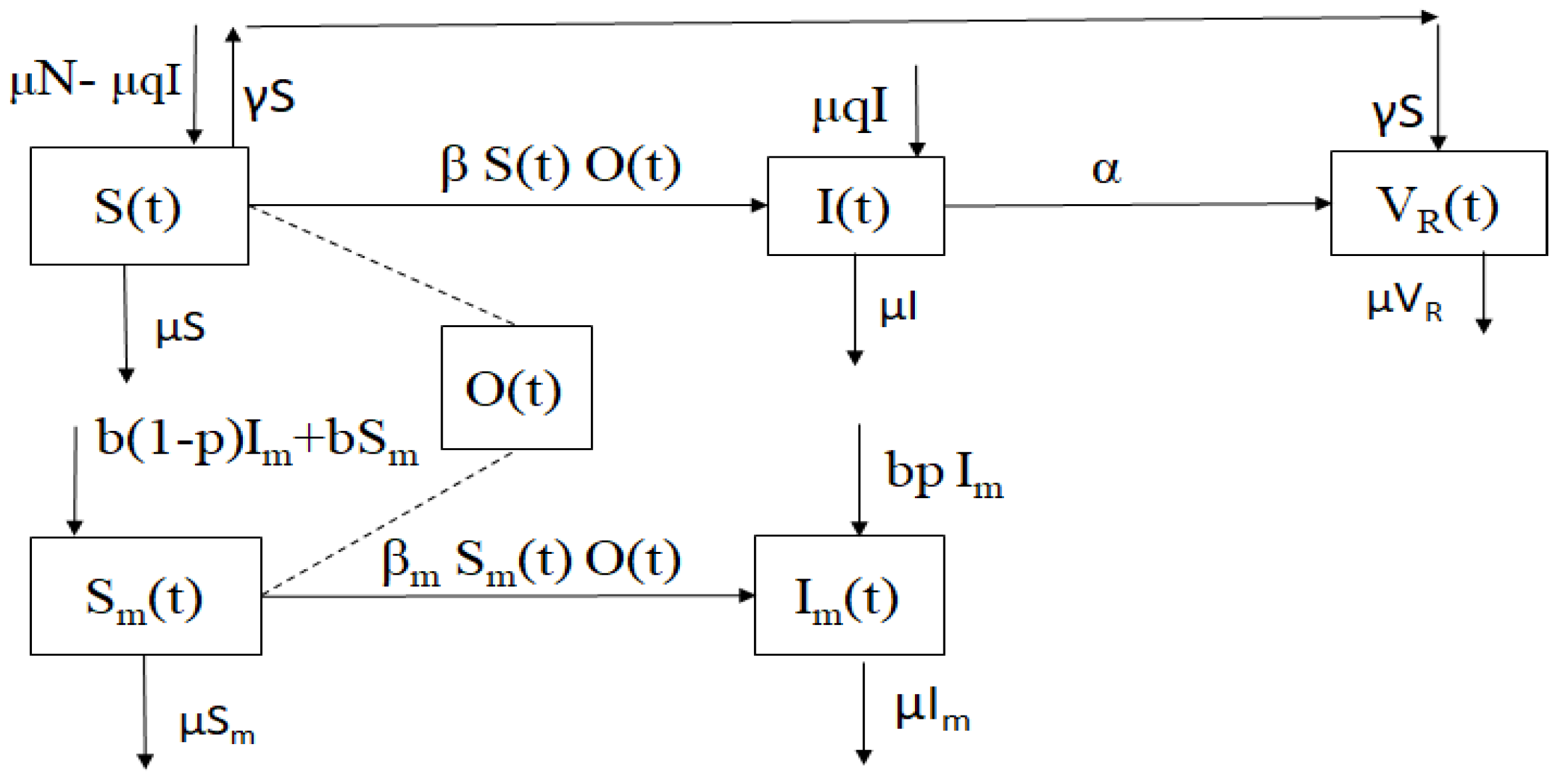
The constructed generalized mathematical model assuming vertical transmission for the mouse and cat populations is provided by the following system:

$$\begin{array}{ccc}\dot{S}\left(t\right)& \hfill =& \mu N-q\mu I\left(t\right)-\beta S\left(t\right)O\left(t\right)-(\gamma +\mu )S\left(t\right),\hfill \\ \dot{I}\left(t\right)& \hfill =& \beta S\left(t\right)O\left(t\right)-\alpha I\left(t\right)-\mu I\left(t\right)+q\mu I\left(t\right),\hfill \\ \dot{V_R}\left(t\right)& \hfill =& \alpha I\left(t\right)+\gamma S\left(t\right)-\mu V_R\left(t\right),\hfill \\ \dot{O}\left(t\right)& \hfill =& kI\left(t\right)-{\mu }_{0}O\left(t\right),\hfill \\ \dot{S_m}\left(t\right)& \hfill =& {\mu }_m{S}_m+{\mu }_m(1-p)I_m-{\beta }_m{S}_m\left(t\right)O\left(t\right)-{\mu }_m{S}_m,\hfill \\ \dot{I_m}\left(t\right)& \hfill =& {\beta }_m{S}_m\left(t\right)O\left(t\right)+{\mu }_{m}p{I}_m-{\mu }_m{I}_m.\hfill \end{array}$$

(1)

The parameter $k>0$ is the production rate of oocysts per infectious cat. The term $q\mu I\left(t\right)$ represents newborn cats that are born with toxoplasmosis due to congenital transmission. Note that there is no vertical transmission in the cat population if $q=0$. Analogously, the term $p\mu I_m\left(t\right)$ represents newborn mice born with toxoplasmosis due to congenital transmission; if $p=0$, there is no vertical transmission in the mouse population. We denote the population of cats by $N\left(t\right)$ and the mouse population by $N_m\left(t\right)$. In order to work with proportions, we scale both the mouse and cat populations. After changing the variables and using a number of simplifications, we obtain the following reduced system:

$$\begin{array}{ccc}\dot{S}\left(t\right)& \hfill =& \mu -q\mu I\left(t\right)-\beta S\left(t\right)O\left(t\right)-(\gamma +\mu )S\left(t\right),\hfill \\ \dot{I}\left(t\right)& \hfill =& \beta S\left(t\right)O\left(t\right)-\alpha I\left(t\right)-\mu I\left(t\right)+q\mu I\left(t\right),\hfill \\ \dot{O}\left(t\right)& \hfill =& kI\left(t\right)-{\mu }_{0}O\left(t\right),\hfill \\ \dot{S_m}\left(t\right)& \hfill =& {\mu }_m(1-p)(1-S_m)-{\beta }_m{S}_m\left(t\right)O\left(t\right).\hfill \end{array}$$

(2)

where $V_R=1-S-I$ and $I_m=1-S_m$. The initial conditions of the subpopulations are as follows:

$$\begin{array}{c}\hfill S_m\left(0\right)\ge 0,O\left(0\right)\ge 0,S\left(0\right)>0,I\left(0\right)\ge 0.\end{array}$$

(3)

The designed model is depicted in Figure 1.

3. Stability Analysis

Here, we qualitatively analyze the mathematical model (2) and obtain the proof of the uniqueness of the solution.

First, we want to demonstrate that the solutions of system (2) are bounded and positive ($\forall t\ge 0$).

Theorem 1. 

When the initial values satisfy (3) and the positivity of the parameters inherent in the system (2) is satisfied, then the solution curves of (2) remain positive and are bounded for $t\ge 0.$

Proof. 

Replacing the inequality $I\left(t\right)\le 1$ in the third equation of (2), it follows that

$$\begin{array}{cc}\hfill \dot{O}\left(t\right)& \le k-{\mu }_{0}O\left(t\right).\hfill \end{array}$$

Thus, if $O\left(0\right)\le {\displaystyle \frac{k}{{\mu }_0}}$, then $O\left(t\right)\le {\displaystyle \frac{k}{{\mu }_0}}$. For the case $O\left(0\right)>{\displaystyle \frac{k}{{\mu }_0}}$, we have $O\left(t\right)<O\left(0\right)$. Taking $B_M=max\left\{O\left(0\right),{\displaystyle \frac{k}{{\mu }_0}}\right\}$, it is then the case that $O\left(t\right)\le B_O$ for all $t\le 0$. In addition, we have

$$\begin{array}{c}\hfill \dot{S}\left(t\right)>-\beta S\left(t\right)B_O-(\mu +\gamma )S\left(t\right),\end{array}$$

which implies that

$$\begin{array}{c}\hfill S\left(t\right)\ge S\left(0\right)exp(-B_{0}t)>0,\end{array}$$

i.e., $S\left(t\right)>0$ for all $t\ge 0$ and $B_0=\beta B_O+\mu +\gamma$. Now, if $t_0>0$ exists such that $I\left(t_0\right)=0,$ $\dot{I}\left(t_0\right)\le 0$, and $I\left(t\right)>0$ for all $t\in [0,t_0)$, we have $0\ge \beta S\left(t_0\right)O\left(t_0\right)$. However, from the equation related to the the variation of $O\left(t\right)$ in model (2), we obtain

$$\begin{array}{c}\hfill \dot{O}\left(t\right)>-{\mu }_{0}O\left(t\right),\forall t\in [0,t_0),\end{array}$$

and

$$\begin{array}{c}\hfill O\left(t_0\right)\ge O\left(0\right)e^{-{\mu }_0{t}_0}>0,\end{array}$$

leading to a contradiction. Then, $I\left(t\right)>0,\forall t>0$. For the rest of state variables, it is sufficient to verify that they are non-negative for $t\ge 0.$ From the first equation of model (2), by applying a comparison theorem [50] it can be seen that

$$\begin{array}{c}\hfill S\left(t\right)\le S\left(0\right)e^{-(\mu +\gamma )t}+\frac{\mu }{\mu +\gamma }(1-e^{-(\mu +\gamma )t}).\end{array}$$

Thus, if $S\left(0\right)\le \frac{\mu }{\mu +\gamma }$, then $S\left(t\right)\le \frac{\mu }{\mu +\gamma }$. In addition, the second equation of system (2) shows that

$$\begin{array}{c}\hfill \dot{I}\left(t\right)\le \frac{\beta \mu k}{(\mu +\gamma ){\mu }_0}-(\alpha +\mu (1-q))I\left(t\right),\end{array}$$

and again, we have

$$\begin{array}{c}\hfill I\left(t\right)\le \frac{\beta \mu k}{(\mu +\gamma ){\mu }_0(\alpha +\mu (1-q))}\end{array}$$

for $I\left(0\right)\le \frac{\beta \mu k}{(\mu +\gamma ){\mu }_0(\alpha +\mu (1-q))}.$ Thus, we investigate model (2) in the next region, as follows:

$$\begin{array}{cc}\hfill {\Omega }_r=\{& (S,I,O,S_m)\in {\mathbb{R}}_{+}^4/0<S\le \frac{\mu }{\mu +\gamma },0\le I\le \frac{\beta \mu k}{(\mu +\gamma ){\mu }_0(\alpha +\mu (1-q))},\hfill \\ & 0<S+I<1,0\le O\le \frac{k}{{\mu }_0},0\le S_m+I_m\le 1\}.\hfill \end{array}$$

(4)

Thus, ${\Omega }_r$ is positively invariant. Note that if $S\left(0\right)>\frac{\mu }{\mu +\gamma }$ the solutions enter ${\Omega }_r$ or $S\left(t\right)$, approaching asymptotically to $\frac{\mu }{\mu +\gamma }$. The same is the case for the rest of the variables. Therefore, the region ${\Omega }_r$ attracts all solutions in ${\mathbb{R}}_{+}^4$. □

Thus, we can study model (2) in ${\Omega }_r$, and model (2) is mathematically well-posed in ${\Omega }_r$.

4. Mathematical Model with Full Vertical Transmission in the Mouse Population

We separate the cases of full vertical transmission ($p=1$) and without vertical transmission ($p\ne 1$) for the mouse population, as their mathematical analyses vary and the public health consequences are different. For the sake of clarity, we present system (2) with $p=1$, which translates to full vertical transmission in the mouse population. Then, we have

$$\begin{array}{ccc}\dot{S}\left(t\right)& \hfill =& \mu -q\mu I\left(t\right)-\beta S\left(t\right)O\left(t\right)-(\gamma +\mu )S\left(t\right),\hfill \\ \dot{I}\left(t\right)& \hfill =& \beta S\left(t\right)O\left(t\right)-\alpha I\left(t\right)-\mu I\left(t\right)+q\mu I\left(t\right),\hfill \\ \dot{O}\left(t\right)& \hfill =& kI\left(t\right)-{\mu }_{0}O\left(t\right),\hfill \\ \dot{S_m}\left(t\right)& \hfill =& -{\beta }_m{S}_m\left(t\right)O\left(t\right).\hfill \end{array}$$

(5)

We begin by studying the stability of the toxoplasmosis-free steady states, assuming full vertical transmission in the mouse population. We then proceed to find the equilibrium points and study their stability.

4.1. Toxoplasmosis-Free Steady State Considering Full Vertical Transmission in Mice

The steady states of epidemiological models are crucial for studying disease dynamics. Such models might have multiple equilibria and periodic solutions. From the generalized mathematical model (5), we can clearly see that infinite steady states are attained when $I=0$ and $O=0$. These steady states are part of a subset of ${\Omega }_r$. Now, we define the following set:

$$J=\left\{(S,I,O,S_m):\left(\frac{\mu }{\mu +\gamma },0,0,S_m^{*}\right)\in {\Omega }_r\right\}.$$

(6)

We name this set the toxoplasmosis-free set. LaSalle’s invariance principle can be used to rule the stability of this set J [50]. As a matter of fact, we can build a Lyapunov function in order to show that all the solutions of the model (5) are attracted to set J when ${\mathcal{R}}_0<1$.

Remark 1. 

The set J that includes all toxoplasmosis-free equilibrium points considers the possibility of toxoplasmosis disease in the mouse population. However, because mice are not able to spread the disease to cats in system (5) with $p=1$, we consider the set J as a toxoplasmosis-free situation.

Remark 2. 

From system 5, we can take the subsystem of the equations where the compartments into which new infectious agents enter are located. Thus, we can compute the matrices V and F that represent the Jacobian matrices of the compartments with new infections evaluated at points $I=0$ and $O=0$. In this way, we have

$$\begin{array}{c}\hfill F=\left[\begin{array}{cc}0& \frac{\mu \beta }{\gamma +\mu }\\ k& 0\end{array}\right]V=\left[\begin{array}{cc}\alpha +\mu -q\mu & 0\\ 0& {\mu }_0\end{array}\right].\end{array}$$

We define the basic reproduction number

$$\begin{array}{c}\hfill {\mathcal{R}}_0=\sqrt{\frac{\mu k\beta }{{\mu }_0\left(\gamma +\mu \right)(\alpha +\mu -q\mu )}},\end{array}$$

(7)

which is obtained by calculating the maximum eigenvalue of the product $F{V}^{-1}$ provided by

$$\begin{array}{c}\hfill F{V}^{-1}=\left[\begin{array}{cc}0& \frac{\mu \beta }{\left(\gamma +\mu \right){\mu }_0}\\ \frac{k}{\alpha +\mu -q\mu }& 0\end{array}\right].\end{array}$$

4.2. Global Stability of Toxoplasmosis-Free Equilibrium Points

First, we show that the set J is the largest invariant set if ${\mathcal{R}}_0<1$ and that for any initial conditions the solutions are attracted to the set J.

Theorem 2. 

When ${\mathcal{R}}_0\le 1,$ the convergence of the solution curves of the model (5) occurs on set J.

Proof. 

We now propose the next function $\mathfrak{S}$,

$$\begin{array}{c}\hfill \mathfrak{S}\left(\mathcal{X}\left(t\right)\right)={\displaystyle \frac{kI\left(t\right)}{{\mathcal{R}}_0^2(\alpha +\mu -q\mu ){\mu }_0}}+{\displaystyle \frac{O\left(t\right)}{{\mu }_0}},\end{array}$$

(8)

where $\mathcal{X}\left(t\right)=\left(S\left(t\right),I\left(t\right),O\left(t\right),S_m\left(t\right)\right)$ and $F^{*}\in J$. Here, $\mathfrak{S}$ is a function such that:

$$\begin{array}{cc}\hfill & \mathfrak{S}\left(F^{*}\right)=0\mathrm{for}\mathrm{all}{F}^{*}\in J;\hfill \\ \hfill & \mathfrak{S}\left(\mathcal{X}\left(t\right)\right)>0\mathrm{for}\mathrm{all}\mathcal{X}\left(t\right)\ne F^{*};\hfill \\ \hfill & \mathfrak{S}\left(\mathcal{X}\left(t\right)\right)\to \infty ,\mathrm{as}∥\mathcal{X}∥\to \infty .\mathrm{Thus},\mathfrak{S}\left(\mathcal{X}\left(t\right)\right)\mathrm{is}\mathrm{radially}\mathrm{unbounded}.\hfill \end{array}$$

(9)

Computing the time derivative of $\mathfrak{S}\left(\mathcal{X}\right(t\left)\right)$ along the trajectories of model (5), from ${\Omega }_r$ it follows that

$$\begin{array}{cc}\hfill {\displaystyle \frac{d\mathfrak{S}\left(\mathcal{X}\right(t\left)\right)}{dt}}=& {\displaystyle \frac{k\dot{I}\left(t\right)}{{\mathcal{R}}_0^2(\alpha +\mu -q\mu ){\mu }_0}}+{\displaystyle \frac{\dot{O}\left(t\right)}{{\mu }_0}}={\displaystyle \frac{k\left(\beta S\right(t\left)O\right(t)-(\alpha +\mu -q\mu \left)I\right(t\left)\right)}{{\mathcal{R}}_0^2(\alpha +\mu -q\mu ){\mu }_0}}+{\displaystyle \frac{kI\left(t\right)-{\mu }_{0}O\left(t\right)}{{\mu }_0}}\hfill \\ \\ \hfill =& \frac{k\beta S\left(t\right)O\left(t\right)-kI\left(t\right)(\alpha +\mu -q\mu )+kI\left(t\right){\mathcal{R}}_0^2(\alpha +\mu -q\mu )-O\left(t\right){\mu }_0{\mathcal{R}}_0^2(\alpha +\mu -q\mu )}{{\mathcal{R}}_0^2(\alpha +\mu -q\mu ){\mu }_0}\hfill \\ \\ \hfill =& \frac{kI\left(t\right)(\alpha +\mu -q\mu )({\mathcal{R}}_0^2-1)+O\left(t\right)(k\beta S\left(t\right)-{\mathcal{R}}_0^2{\mu }_0(\alpha +\mu -q\mu ))}{{\mathcal{R}}_0^2(\alpha +\mu -q\mu ){\mu }_0}\hfill \\ \\ \hfill \le & \frac{kI\left(t\right)(\alpha +\mu -q\mu )({\mathcal{R}}_0^2-1)+O\left(t\right)\left({\displaystyle \frac{k\beta \mu }{\mu +\gamma }}-{\mathcal{R}}_0^2{\mu }_0(\alpha +\mu -q\mu )\right)}{{\mathcal{R}}_0^2(\alpha +\mu -q\mu ){\mu }_0}\hfill \\ \\ \hfill =& \frac{kI\left(t\right)(\alpha +\mu -q\mu )({\mathcal{R}}_0^2-1)}{{\mathcal{R}}_0^2(\alpha +\mu -q\mu ){\mu }_0}.\hfill \end{array}$$

Thus, when ${\mathcal{R}}_0\le 1,$ it is the case that ${\displaystyle \frac{d\mathfrak{S}\left(\mathcal{X}\right(t\left)\right)}{dt}}\le 0$ and ${\displaystyle \frac{d\mathfrak{S}\left(\mathcal{X}\right(t\left)\right)}{dt}}=0$ iff $I\left(t\right)=0$ and $O\left(t\right)=0$. Therefore, the set

$$\begin{array}{c}\hfill {\mathfrak{S}}_{F^{*}}=\left\{\mathcal{X}\left(t\right)\in {\Omega }_r:{\displaystyle \frac{d\mathfrak{S}\left(\mathcal{X}\right(t\left)\right)}{dt}}=0\right\}\end{array}$$

is simply the set J. Per LaSalle’s invariance principle, we find that the limit set of all solutions belongs to the largest time-invariant set $J\in {\Omega }_r$ whenever ${\mathcal{R}}_0\le 1$. □

4.3. Toxoplasmosis-Endemic Steady State

The biological toxoplasmosis-endemic steady states can be obtained by solving the algebraic system

$$\begin{array}{ccc}0& \hfill =& \mu -q\mu I^{*}-\beta S^{*}{O}^{*}-(\gamma +\mu )S^{*},\hfill \\ 0& \hfill =& \beta S^{*}{O}^{*}-\alpha I^{*}-\mu I^{*}+q\mu I^{*},\hfill \\ 0& \hfill =& k{I}^{*}-{\mu }_0{O}^{*},\hfill \\ 0& \hfill =& -{\beta }_m{S}_m^{*}{O}^{*}.\hfill \end{array}$$

(10)

We denote the toxoplasmosis-endemic point by

$$\begin{array}{c}\hfill E_0^{*}=\left(S^{*},I^{*},O^{*},S_m^{*}\right).\end{array}$$

(11)

Then, from (10), we find that $S_m^{*}=0$, as $O^{*}\ne 0$. Therefore, the components of the toxoplasmosis-endemic steady state are

$$\begin{array}{cc}\hfill S^{*}=& {\displaystyle \frac{{\mu }_0(\alpha +\mu -q\mu )}{\beta k}},\hfill \\ \hfill I^{*}=& \frac{\mu \beta k-(\gamma +\mu ){\mu }_0(\alpha +\mu -q\mu )}{\beta k\left(\mu q+\alpha +\mu -q\mu \right)},\hfill \\ \hfill O^{*}=& \frac{\mu \beta k-(\gamma +\mu ){\mu }_0(\alpha +\mu -q\mu )}{\beta \left(\mu q+\alpha +\mu -q\mu \right){\mu }_0},\hfill \\ \hfill S_m^{*}=& 0.\hfill \end{array}$$

(12)

Using ${\mathcal{R}}_0$, we find that the endemic point $E_0^{*}$ is provided as follows:

$$\begin{array}{cc}\hfill S^{*}=& {\displaystyle \frac{\mu }{{\mathcal{R}}_0^2(\mu +\gamma )}},\hfill \\ \hfill I^{*}=& {\displaystyle \frac{{\mu }_0(\gamma +\mu )(\alpha +\mu -q\mu )({\mathcal{R}}_0^2-1)}{\beta k\left(\mu q+\alpha +\mu -q\mu \right)}},\hfill \\ \hfill O^{*}=& {\displaystyle \frac{(\gamma +\mu )(\alpha +\mu -q\mu )({\mathcal{R}}_0^2-1)}{\beta k\left(\mu q+\alpha +\mu -q\mu \right)}},\hfill \\ \hfill S_m^{*}=& 0.\hfill \end{array}$$

(13)

The endemic steady state $E_0^{*}$ is biologically appropriate if $\mu \beta k-{\mu }_0(\gamma +\mu )(\alpha +\mu -q\mu )>0$. If ${\mathcal{R}}_0=1$, this endemic equilibrium becomes part of the set J composed by the toxoplasmosis-free steady states. As a matter of fact, the endemic and disease-free equilibrium points collide when ${\mathcal{R}}_0=1$. The characteristic polynomial is provided by

$$P\left(\lambda \right)=\left|\begin{array}{cccc}-\beta O^{*}-\mu -\gamma -\lambda & -q\mu & -\beta S^{*}& 0\\ \beta O^{*}& -\alpha -\mu +q\mu -\lambda & \beta S^{*}& 0\\ 0& k& -{\mu }_0-\lambda & 0\\ 0& 0& -{\beta }_m{S}_m^{*}& -{\beta }_m{O}^{*}-\lambda \end{array}\right|$$

Then, the eigenvalue $\lambda =-{\beta }_m{O}^{*}$ is clearly negative. To compute the further eigenvalues, we simply need to compute the roots of

$$\begin{array}{cc}\hfill & {\lambda }^3+(\beta O^{*}+\alpha +\gamma +{\mu }_0+\mu (2-q)){\lambda }^2\hfill \\ \hfill & +(O^{*}\alpha \beta +O^{*}\beta {\mu }_0+O^{*}\beta {\mu }_c-k\beta S^{*}-\gamma \mu q-{\mu }_0\mu q-{\mu }^{2}q+\alpha \gamma +\alpha {\mu }_0+\mu \alpha +\gamma {\mu }_0+\gamma \mu +2{\mu }_0\mu +{\mu }^2)\lambda \hfill \\ \hfill & +O^{*}\alpha \beta {\mu }_0+O^{*}\beta {\mu }_0\mu -S^{*}\beta k(\gamma +\mu )-\gamma {\mu }_0\mu q-{\mu }_0{\mu }^{2}q+\alpha \gamma {\mu }_0+\alpha {\mu }_0\mu +\gamma {\mu }_0\mu +{\mu }_0{\mu }^2=0.\hfill \end{array}$$

(14)

We can rewrite this characteristic equation as

$$\begin{array}{c}\hfill {\lambda }^3+A{\lambda }^2+B\lambda +C=0\end{array}$$

(15)

where

$$\begin{array}{cc}\hfill A& =O^{*}\beta +\alpha +\gamma +{\mu }_0+\mu (2-q)=\frac{\mathcal{R}}{\alpha +\mu }+\alpha +\gamma +{\mu }_0+\mu (2-q),\hfill \\ \hfill B& =\frac{\mathcal{R}{\mu }_0}{\alpha +\mu }+\mathcal{R}+{\mu }_0\mu +\alpha \gamma +\mu \alpha +\gamma {\mu }_0+\gamma \mu (1-q)+(1-q){\mu }^2,\hfill \\ \hfill C& ={\mu }_0\beta O^{*}(\mu +\alpha )={\mu }_0\mathcal{R}.\hfill \end{array}$$

Here, $\mathcal{R}=(\mu +\gamma )(\alpha +\mu -\mu q)({\mathcal{R}}_0^2-1)>0$, because ${\mathcal{R}}_0>1$. Per the Routh–Hurwitz theorem [51], we can conclude that all the eigenvalues have negative real parts if $AB>C$ and $A,C$ are positive; note that $A,B,C>0$. As such, we can obtain

$$\begin{array}{cc}\hfill AB-C& =\left(\frac{\mathcal{R}}{\alpha +\mu }+\alpha +\gamma +{\mu }_0+\mu (2-q)\right)(\frac{\mathcal{R}{\mu }_0}{\alpha +\mu }+\mathcal{R}+{\mu }_0\mu +\alpha \gamma +\mu \alpha +\gamma {\mu }_0\hfill \\ \hfill & +\gamma \mu (1-q)+(1-q){\mu }^2)-{\mu }_0\mathcal{R}\hfill \\ \hfill & =\left(\frac{\mathcal{R}}{\alpha +\mu }+\alpha +\gamma +{\mu }_0+\mu (2-q)\right)(\frac{\mathcal{R}{\mu }_0}{\alpha +\mu }+{\mu }_0\mu +\alpha \gamma +\mu \alpha +\gamma {\mu }_0\hfill \\ & +\gamma \mu (1-q)+(1-q){\mu }^2)+\left(\frac{\mathcal{R}}{\alpha +{\mu }_c}+\alpha +\gamma +{\mu }_0+\mu (2-q)\right)\mathcal{R}-\mathcal{R}{\mu }_0>0\hfill \end{array}$$

when ${\mathcal{R}}_0>1.$ Thus, all the eigenvalues are located in the left-half plane. Accordingly, the theorem below is proven.

Theorem 3. 

For ${\mathcal{R}}_0>1$, the stationary toxoplasmosis endemic point $E_0^{*}$ is locally asymptotically stable in ${\Omega }_r\backslash J$.

4.4. Global Stability of the Toxoplasmosis-Endemic Equilibrium Point

First, let us examine the global stability of the toxoplasmosis-endemic point $E_0^{*}$. We propose the following theorem:

Theorem 4. 

The toxoplasmosis-endemic steady state $E_0^{*}$ of model (5) is global asymptotically stable in ${\Omega }_r\backslash J$ whenever ${\mathcal{R}}_0>1$.

Proof. 

We define the function $\mathcal{L}$ as

$$\begin{array}{c}\hfill \mathcal{L}\left(\mathcal{X}\left(t\right)\right)=S_m\left(t\right),\end{array}$$

(16)

which complies with (9). Then,

$${\displaystyle \frac{d\mathcal{L}\left(\mathcal{X}\right(t\left)\right)}{dt}}=-{\beta }_m{S}_m\left(t\right)O\left(t\right).$$

Therefore, ${\displaystyle \frac{d\mathcal{L}\left(\mathcal{X}\right(t\left)\right)}{dt}}\le 0$ and ${\displaystyle \frac{d\mathcal{L}\left(\mathcal{X}\right(t\left)\right)}{dt}}=0$ if and only if $S_m\left(t\right)=0$ or $O\left(t\right)=0.$ Following LaSalle’s invariance principle, the toxoplasmosis endemic equilibrium $E_0^{*}$ is globally asymptotically stable with respect to ${\Omega }_0\backslash J$ if ${\mathcal{R}}_0>1.$ □

This stability result implies that system (5) approaches the toxoplasmosis endemic equilibrium point $E_0^{*}$ for ${\mathcal{R}}_0>1$ and for any initial conditions.

5. Mathematical Model without Full Vertical Transmission in the Mouse Population

In this section, we consider the mathematical model (2) without full vertical transmission in the mouse population, i.e., $0\le p<1$. From the previous section, we know that toxoplasmosis cannot be eradicated from the mouse population due to full vertical transmission. Now, we consider the case without full vertical transmission in the mouse population ($0\le p<1$). The reason for considering this separate case is that, as will be seen, it is possible to eradicate toxoplasmosis from both the cat and mouse populations if there is not full vertical transmission. Moreover, there are only two steady states here instead of infinitely many. Proceeding with the analysis of the mathematical model without full vertical transmission in the mouse population, the model under investigation here is provided by system (2) with $0<p<1$.

5.1. Stability Analysis of the Toxoplasmosis-Free Equilibrium Point

We denote the total toxoplasmosis-free equilibrium point of model (2) as

$$F_0^{*}=(S^{*},I^{*},O^{*},S_m^{*})=\left({\displaystyle \frac{\mu }{\mu +\gamma }},0,0,1\right).$$

Note that the whole population of mice is susceptible. There are no oocysts and no infected cats. We call this steady state a total toxoplasmosis-free state, as none of the subpopulations are infected. This case is different from the one in which there is full vertical transmission in the mouse population. Next, we proceed to study the local stability of the total toxoplasmosis-free equilibrium point $F_0^{*}$. The local stability of $F_0^{*}$ can be examined by analyzing the eigenvalues of $J\left(F_0^{*}\right)$. Evaluating the Jacobian of Equation (2) at $F_0^{*}$, we have

$$J\left(F_0^{*}\right)=\left(\begin{array}{cccc}-\mu -\gamma & -q\mu & -\frac{\beta \mu }{\mu +\gamma }& 0\\ 0& q\mu -\mu -\alpha & \frac{\beta \mu }{\mu +\gamma }& 0\\ 0& k& -{\mu }_0& 0\\ 0& 0& -{\beta }_m& -{\mu }_m(1-p)\end{array}\right).$$

By calculating the eigenvalues of the matrix $J\left(F_0^{*}\right)$, we obtain the characteristic equation, which can be factored as

$$\begin{array}{cc}\hfill & \frac{\left({\mu }_{m}p-\lambda -{\mu }_m\right)\left(\gamma +\lambda +\mu \right)}{\gamma +\mu }\hfill \\ \hfill & *\left(\left(\gamma +\mu \right){\lambda }^2+\left(\mu +\gamma \right)\left((1-q)\mu +\alpha +{\mu }_0\right)\lambda +(\mu +\gamma ){\mu }_0\left((1-q)\mu +\alpha \right)-\mu k\beta \right)=0.\hfill \end{array}$$

We can obtain two eigenvalues, ${\lambda }_1=-\mu -\gamma$ and ${\lambda }_2=-{\mu }_m(1-p)$. To compute further eigenvalues, we can find the roots of

$$p\left(\lambda \right)={\lambda }^2+(\alpha +{\mu }_0+\mu (1-q))\lambda +{\mu }_0(\alpha +\mu (1-q))(1-{\mathcal{R}}_0),$$

(17)

where ${\mathcal{R}}_0={\displaystyle \frac{\mu \beta k}{{\mu }_0(\gamma +\mu )(\alpha +\mu -q\mu )}}.$ The polynomial in Equation (17) can be rewritten as

$$p\left(\lambda \right)={\lambda }^2+a_1\lambda +a_0,$$

(18)

where $a_1=\alpha +{\mu }_0+\mu (1-q)>0$ and $a_0=\mu (1-q)(1-{\mathcal{R}}_0)>0$. Then, according to the Routh–Hurwitz criterion, all the roots of the polynomial $p\left(\lambda \right)$ have a negative real part. Hence, the total toxoplasmosis-free steady state $F_0^{*}$ is locally asymptotically stable. Now, we proceed to examine the global stability of the toxoplasmosis-free steady state $F_0^{*}$. Using the same reproduction number ${\mathcal{R}}_0$ and the same Lyapunov function provided in Equation (16), we can prove the global stability of the toxoplasmosis-free steady state $F_0^{*}$. Note that in this case the largest time invariant set is reduced to $F_0^{*}\in {\Omega }_r$ if ${\mathcal{R}}_0\le 1$.

5.2. Stability Analysis of the Toxoplasmosis Endemic Equilibrium Point

Using Equation (17), we can see that the steady state $F_0^{*}$ is unstable when ${\mathcal{R}}_0>1.$ Thus, the solutions of model (2) might converge to endemic equilibrium points when ${\mathcal{R}}_0>1$. Examining the stability of the endemic steady state, we can find the endemic state by solving the following system:

$$\begin{array}{ccc}0& \hfill =& \mu -q\mu I^{*}-\beta S^{*}{O}^{*}-(\gamma +\mu )S^{*},\hfill \\ 0& \hfill =& \beta S^{*}{O}^{*}-\alpha I^{*}-\mu I^{*}+q\mu I^{*},\hfill \\ 0& \hfill =& k{I}^{*}-{\mu }_0{O}^{*},\hfill \\ 0& \hfill =& -{\beta }_m{S}_m^{*}{O}^{*}+{\mu }_m(1-p)(1-S_m^{*}).\hfill \end{array}$$

(19)

The biologically realistic endemic point is the positive solution of system (19), and is denoted by

$$\begin{array}{c}\hfill E_1^{*}=\left(S^{*},I^{*},O^{*},S_m^{*}\right),\end{array}$$

(20)

where

$$\begin{array}{cc}\hfill & S^{*}={\displaystyle \frac{{\mu }_0(\alpha +\mu -q\mu )}{\beta k}},\hfill \\ \hfill & I^{*}={\displaystyle \frac{\mu \beta k-{\mu }_0(\gamma +\mu )(\alpha +\mu -q\mu )}{\beta k(\mu +\alpha )}},\hfill \\ \hfill & O^{*}={\displaystyle \frac{\mu \beta k-{\mu }_0(\gamma +\mu )(\alpha +\mu -q\mu )}{\beta {\mu }_0(\mu +\alpha )}},\hfill \\ \hfill & S_m^{*}={\displaystyle \frac{{\mu }_m\beta {\mu }_0(1-p)(\mu +\alpha )}{{\mu }_m\beta {\mu }_0(1-p)(\mu +\alpha )-{\beta }_m{\mu }_0(\alpha +\mu (1-q))(\mu +\gamma )+\beta {\beta }_{m}k\mu }}.\hfill \end{array}$$

(21)

Now, using ${\mathcal{R}}_0,$ the unique endemic equilibrium point $E_1^{*}$ can be rewritten as follows:

$$\begin{array}{cc}\hfill & S^{*}={\displaystyle \frac{\mu }{{\mathcal{R}}_0^2(\mu +\gamma )}},\hfill \\ \hfill & I^{*}={\displaystyle \frac{{\mu }_0(\gamma +\mu )(\alpha +\mu -q\mu )({\mathcal{R}}_0^2-1)}{\beta k(\mu +\alpha )}},\hfill \\ \hfill & O^{*}={\displaystyle \frac{(\gamma +\mu )(\alpha +\mu -q\mu )({\mathcal{R}}_0^2-1)}{\beta (\mu +\alpha )}},\hfill \\ \hfill & S_m^{*}={\displaystyle \frac{{\mu }_m\beta {\mu }_0(1-p)(\mu +\alpha )}{{\mu }_m\beta {\mu }_0(1-p)(\mu +\alpha )+{\beta }_m{\mu }_0(\alpha +\mu (1-q))(\mu +\gamma )}}({\mathcal{R}}_0^2-1).\hfill \end{array}$$

(22)

It can be observed that we obtain a practical endemic equilibrium $E_1^{*}$ if $\mu \beta k-{\mu }_0(\gamma +\mu )(\alpha +\mu -q\mu )>0$. Note that this previous condition is equivalent to having ${\mathcal{R}}_0>1$. Further, note that the endemic equilibrium point $E_1$ depends on the respective generalized proportions of vertical transmission in the cat and mouse populations. Calculating the Jacobian at $E_1^{*}$, we obtain

$$P\left(\lambda \right)=\left|\begin{array}{cccc}-\beta O^{*}-\mu -\gamma -\lambda & -q\mu & -\beta S^{*}& \hfill 0\\ \beta O^{*}& -\alpha -\mu +q\mu -\lambda & \beta S^{*}& \hfill 0\\ 0& k& -{\mu }_0-\lambda & \hfill 0\\ 0& 0& -{\beta }_m{S}_m^{*}& \hfill -{\beta }_m{O}^{*}-(1-p){\mu }_m-\lambda \end{array}\right|$$

Clearly, $\lambda =-{\beta }_m{O}^{*}-(1-p){\mu }_m$ is a negative eigenvalue. The other eigenvalues are the zeros in Equation (14). Thus, using the Routh–Hurwitz theorem, we can find that the zeros in Equation (14) are all located on the left half of the complex plane. Therefore, we obtain the following theorem.

Theorem 5. 

The stationary endemic point $E_1^{*}$ is locally asymptotically stable when the value of the parameter ${\mathcal{R}}_0$ is greater than 1.

Note that the toxoplasmosis endemic equilibrium points of systems (2) and (5) are different. A larger value of the proportion p allows system (5) to reach an endemic steady state with more infected mice. The effect of the proportion q is similar for systems (2) and (5). A larger value of q indicates larger infected populations of cats and mice. Thus, the proportion of q related to vertical transmission in cats is more crucial for the prevalence of toxoplasmosis. This has important consequences from a public health viewpoint.

6. Numerical Simulations of Different Scenarios

In this section, we present a variety of numerical simulations using mathematical model (2). We vary the values of the parameters in order to provide different scenarios. We consider simulations with ${\mathcal{R}}_0<1$ and ${\mathcal{R}}_0>1$ in order to corroborate the theoretical stability analysis presented in the previous section. We vary the initial conditions of the subpopulations in order to take into account conditions both near to and far from the steady states. We mostly rely on the baseline parameter values shown in

Table 1. Baseline values for the parameters and subpopulations.

Parameter	Description	Value
$\mu$	Death and birth rates (cats)	$1/260$ (1/weeks) [52]
$\alpha$	Shedding period	$1/2$ (1/weeks) [4]
${\mu }_0$	Clearance rate	$1/26$ (1/day) [4,36]
k	Oocysts per day (cat)	$20\times {10}^6$ (1/day) [53]
$\beta$	Transmission rate	varying
${\beta }_m$	Transmission rate	$0.1\times {10}^{-8}$
$\gamma$	Vaccination rate	varying
Subpopulations	Description	Initial values
S	Susceptible cats	0.45 [36,54,55]
I	Infected cats	1/130 [36,54,55]
$V_R$	Vaccinated/Recovered	$1-S\left(0\right)-V\left(0\right)$
O	Occysts	$5.92\times {10}^6$
$S_m$	Susceptible mice (proportion)	0.9
$I_m$	Infected mice (proportion)	0.1

.

6.1. Toxoplasmosis-Free Scenario (${\mathcal{R}}_0<1$)

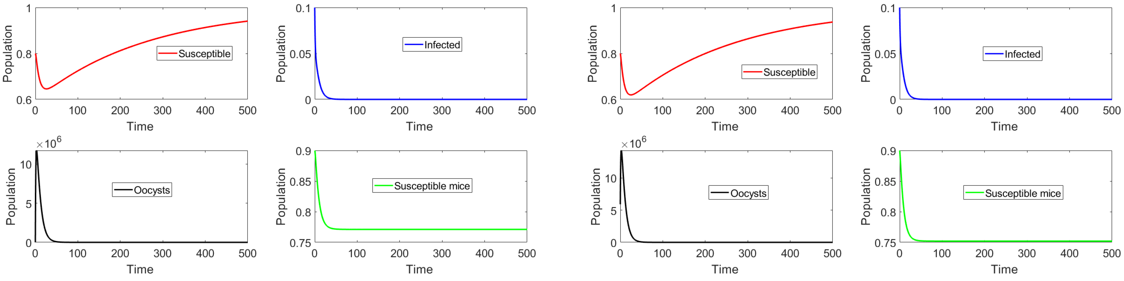
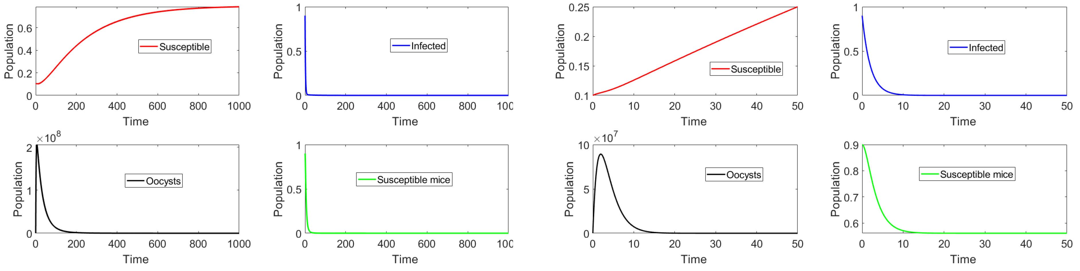
Initially, we consider the case such that ${\mathcal{R}}_0<1$ with initial conditions close to and far from set J. Figure 2 shows the dynamics of the different classes. On the left side, it can be observed that the subpopulation of infectious cats approaches zero when the subpopulations begin near the total toxoplasmosis-free equilibrium point. On the right-hand side, the initial amount of oocysts is a very large number (i.e., far from set J); nevertheless, the system approaches one of the toxoplasmosis-free steady states contained in set J. Note that the oocysts and infected cat populations become extinct here, as ${\mathcal{R}}_0<1$. This simulation result supports the theoretical stability analysis results. Additional simulations were performed, though the results are not shown here. In Figure 3, the main difference is that all the components of the initial conditions are far from the toxoplasmosis-free situation. We considered two vaccination cases, namely, with and without vaccination. On the right-hand side, the case with no vaccination is considered, together with a larger death/clearance rate ${\mu }_0$. Note that in the latter case there is a larger population of susceptible mice due to a smaller amount of oocysts at the steady state. Thus, it can be seen that it is feasible for the disease to disappear despite a low vaccination rate. Again, the numerical simulations support the theoretical stability analysis in the previous section.

6.2. Toxoplasmosis Endemic Scenario (${\mathcal{R}}_0>1$)

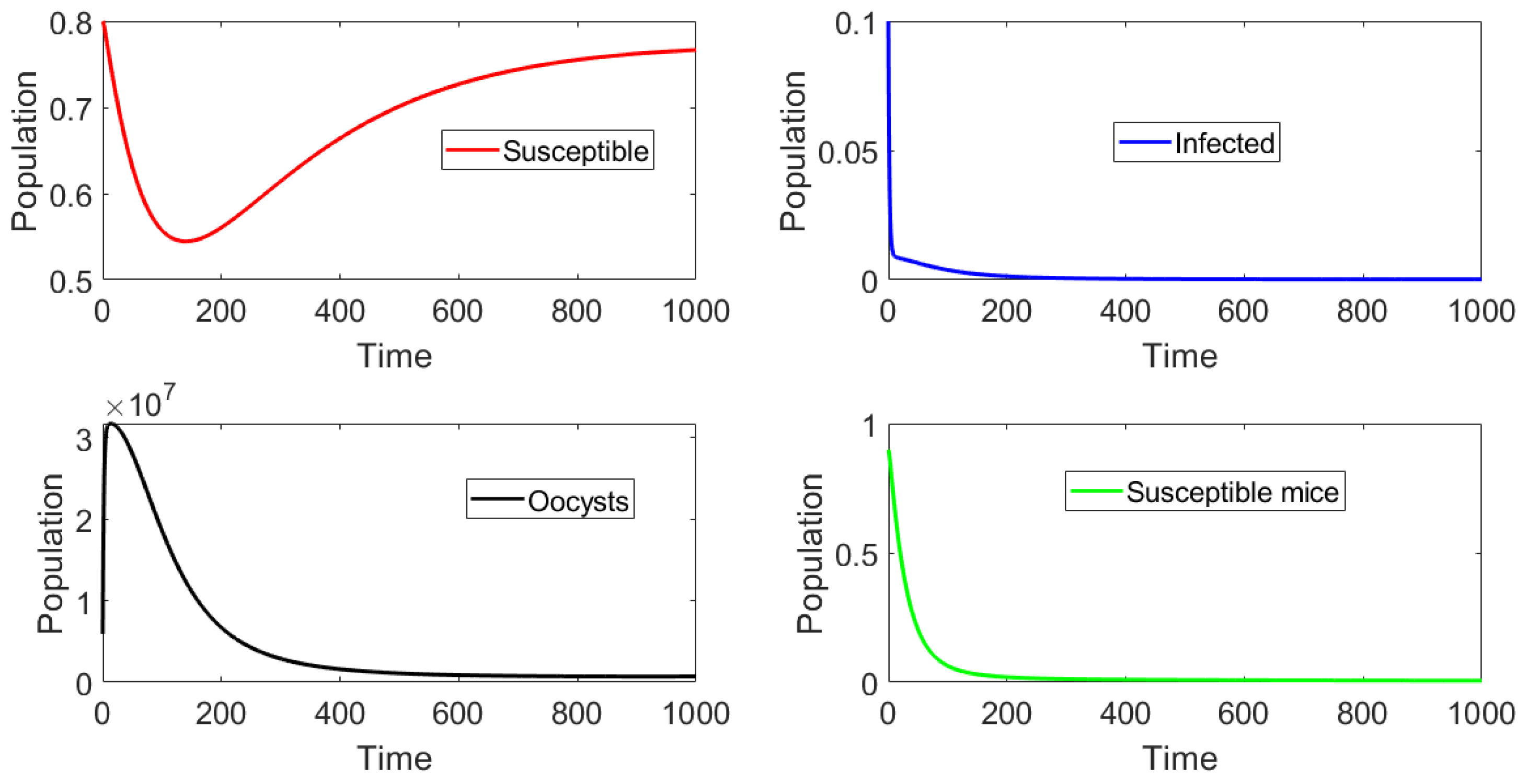
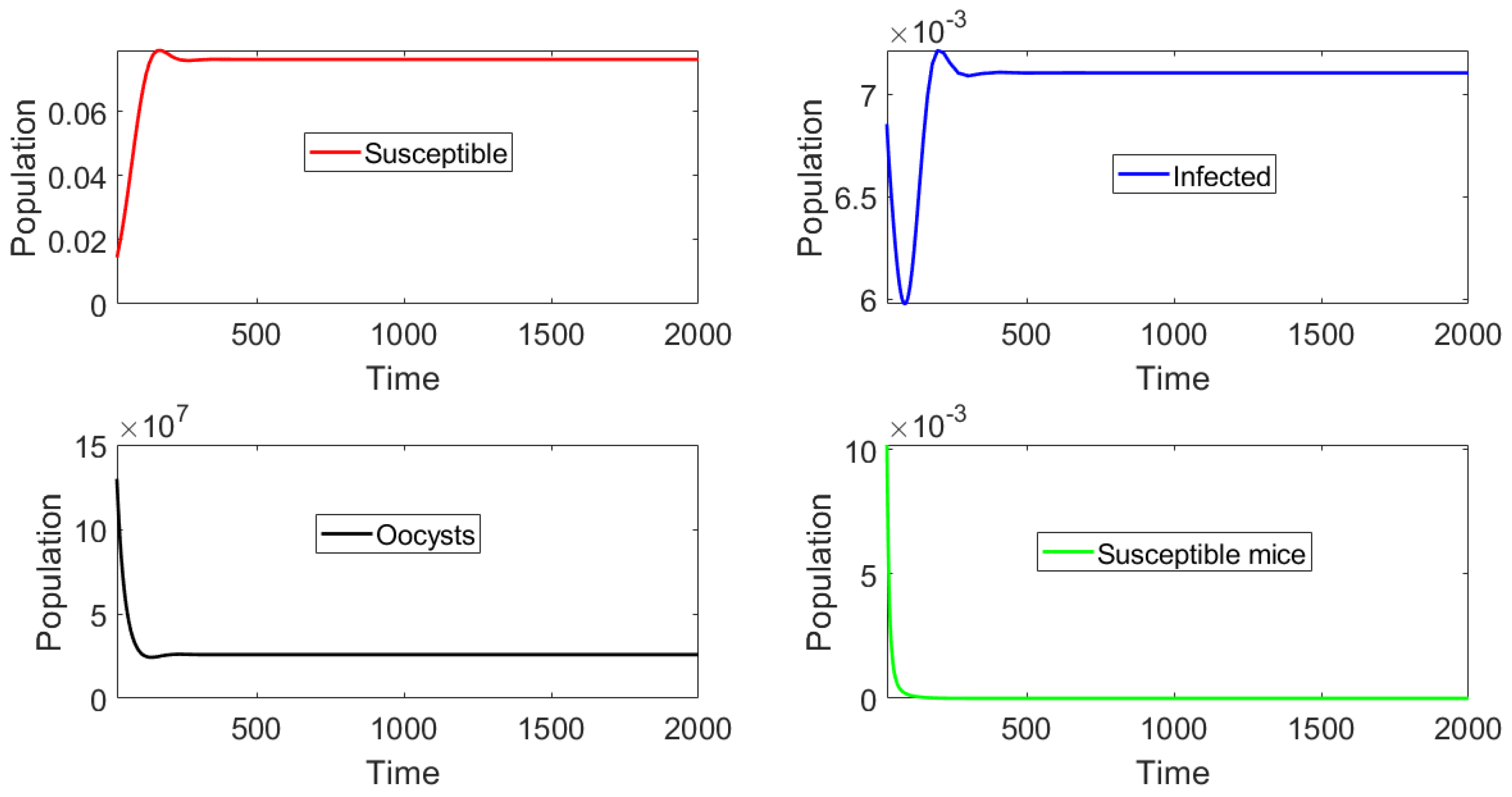
In this section we present the results of in silico simulations, where the parameter values are such that the basic reproduction number ${\mathcal{R}}_0>1$. Figure 4 shows that toxoplasmosis becomes endemic and the subpopulations approach the toxoplasmosis endemic point $E_0^{*}$. The full transient behavior of system (2) can be observed. The system reaches an endemic steady state where $I_m$ and $O\left(t\right)$ do not vanish. Thus, the long term behavior ($t\to \infty$) is the endemic steady state. The number of infected cats is low due to the fact that ${\mathcal{R}}_0=1.04$, i.e., barely above one. If we increase ${\mathcal{R}}_0$, then the infectious population of cats increases. Moreover, the population of susceptible mice $S_m\left(t\right)$ vanishes, due to the oocysts always being present in the environment and to the fact that vertical transmission ($p\ne 0$) is considered in the mouse population.

Finally, an additional numerical simulation with a larger basic reproduction number can be used to examine its effects on the different populations. In particular, we consider no vaccination ($\gamma =0$) and set the parameter $\beta$ such that ${\mathcal{R}}_0\approx 13$. In addition, the initial subpopulations are set to be distant from the toxoplasmosis-free equilibria. Figure 5 shows that the number of infectious cats increases when the basic reproduction number increases. Analogously, the same happens with respect to the quantity of oocysts at the toxoplasmosis endemic equilibrium point. It is apparent that all of these simulation results support our theoretical stability analysis.

7. Conclusions

We created a generalized epidemiological mathematical model to examine and investigate toxoplasmosis disease dynamics. The model incorporates the mouse as an intermediate host for T. gondii and the cat as the primary host. We considered generalized proportions for the vertical transmission in both the cat and mouse populations. We focused on finding the circumstances under which toxoplasmosis can be eradicated. We performed a stability analysis in order to reveal the evolution of toxoplasmosis disease in the cat and mouse populations. We calculated the basic reproduction number ${\mathcal{R}}_0$, and found that it is a crucial secondary parameter that dictates the evolution of toxoplasmosis. Furthermore, this parameter ${\mathcal{R}}_0$ impacts the steady state related to the populations and the disease status. We found that vertical transmission in cats affects the basic reproduction number ${\mathcal{R}}_0$ and that this aspect is crucial for the evolution of toxoplasmosis. The toxoplasmosis-free steady state is globally stable when ${\mathcal{R}}_0<1$ and there is no full vertical transmission, meaning that toxoplasmosis is eradicated regardless of the initial population conditions. However, if we consider the very particular scenario in which there is full vertical transmission in the mouse subpopulation, then the population of infected mice $I_m\left(t\right)$ does not vanish, while both the level of infection in the cat population and the quantity of oocysts in the environment approaches zero. On the other hand, we have proven the uniqueness of the only biologically realistic toxoplasmosis endemic steady state when ${\mathcal{R}}_0>1$ and demonstrated that this endemic state is stable whenever ${\mathcal{R}}_0>1$. Moreover, the population of susceptible mice $S_m\left(t\right)$ vanishes, as the oocysts are always present and continue to infect cats. In summary, we were able to determine the conditions in which the single-celled parasite T. gondii can disappear from the environment. We found that the intermediate host (the mouse population) does not affect the likelihood of achieving the toxoplasmosis-free steady state. Based on the constructed model, the crucial population for eradication of the T. gondii parasite is the definitive host, that is, the cat population.

We performed several numerical simulations that supported the theoretical stability analysis obtained in this research. We used a number of parameter values that involved a degree of uncertainty. We varied a few of these parameters (such as the transmission rate) in order to determine dynamic aspects that were predicted from the theoretical results. This research is useful for health institutions, as it can assist in understanding the main factors that affect the dynamics of toxoplasmosis.

Finally, we need to mention several limitations of this research. A number of of these are common to mathematical modeling studies of epidemics. Fist, accurate estimations of certain parameter values are not yet available. Another important limitation is that the model does not incorporate all intermediate hosts. For instance, it has been documented that birds and sheep can act as intermediate hosts. Including more intermediate hosts would, of course, make the theoretical analysis more difficult. We expect to include these other hosts in future work. Additional limitations include the fact that cat and mouse populations were assumed to be constant. This could be unrealistic in many places around the world. Furthermore, we did not include the prey–predator relationship between the populations, which could be a factor in the eradication of toxoplasmosis. All these limitations are natural in epidemiological models, and are more relevant for multiple hosts. Nevertheless, this research provides deeper insight and understanding of toxoplasmosis dynamics. For instance, based on the analytical form of the basic reproduction number ${\mathcal{R}}_0$, it can be deduced that the prevalence of toxoplasmosis can be reduced by implementing vaccination programs for cats and/or designing a process to reduce the amount of oocysts in the environment.

References

- Reyes-Lizano, L.; Chinchilla-Carmona, M.; Guerrero-Bermúdez, O.; Arias-Echandi, M.; Castro-Castillo, A. Trasmisión de Toxoplasma gondii en Costa Rica: Un concepto actualizado. Acta Méd. Costarric. 2001, 43, 36–38. (In Spanish) [Google Scholar] [CrossRef]
- Beaver, P.; Jung, R.; Cupp, E. Clinical Parasitology, 9th ed.; Lea & Febiger: Philadelphia, PA, USA, 1984. [Google Scholar]
- Markell, E.; Voge, M.; David, J. Parasitología Médica; Mc Graw-Hill: Madrid, Spain, 1990. (In Spanish) [Google Scholar]
- Dubey, J. Duration of Immunity to Shedding of Toxoplasma gondii Oocysts by Cats. J. Parasitol. 1995, 81, 410–415. [Google Scholar] [CrossRef]
- Sibley, L.; Boothroyd, J. Virulent strains of Toxoplasma gondii comprise a single clonal lineage. Nature 1992, 359, 82–85. [Google Scholar] [CrossRef]
- Sunquist, M.; Sunquist, F. Wild Cats of the World; University of Chicago Press: Chicago, IL, USA, 2002. [Google Scholar]
- CDC. Center for Disease Control and Prevention, Toxoplasmosis. 2022. Available online: https://www.cdc.gov/parasites/toxoplasmosis/ (accessed on 10 March 2022).
- Dubey, J.P. The history of Toxoplasma gondii—The first 100 years. J. Eukaryot. Microbiol. 2008, 55, 467–475. [Google Scholar] [CrossRef]
- Lappin, M. Feline toxoplasmosis. Practice 1999, 21, 578–589. [Google Scholar] [CrossRef]
- Aramini, J.; Stephen, C.; Dubey, J.P.; Engelstoft, C.; Schwantje, H.; Ribble, C.S. Potential contamination of drinking water with Toxoplasma gondii oocysts. Epidemiol. Infect. Camb. Univ. Press 1999, 122, 305–315. [Google Scholar] [CrossRef]
- Dubey, J.P.; Thayer, D.W.; Speer, C.A.; Shen, S.K. Effect of gamma irradiation on unsporulated and sporulated Toxoplasma gondii oocysts. Int. J. Parasitol. 1998, 28, 369–375. [Google Scholar] [CrossRef]
- Mead, P.; Slutsker, L.; Dietz, V.; McCaig, L.; Bresee, J.S.; Shapiro, C.; Griffin, P.; Tauxe, R. Food-related illness and death in the United States. Emerg. Infect. Dis. 1999, 5, 607–625. [Google Scholar] [CrossRef]
- Dubey, J.; Frenkel, J. Feline toxoplasmosis from acutely infected mice and the development of Toxoplasma cysts. J. Protozool. 1976, 23, 537–546. [Google Scholar] [CrossRef]
- Dabritz, H.; Conrad, P.A. Cats and Toxoplasma: Implications for public health. Zoonoses Public Health 2010, 57, 34–52. [Google Scholar] [CrossRef]
- Torda, A. Toxoplasmosis. Are cats really the source? Aust. Fam. Physician 2001, 30, 743–747. [Google Scholar]
- Turner, M.; Lenhart, S.; Rosenthal, B.; Zhao, X. Modeling effective transmission pathways and control of the world’s most successful parasite. Theor. Popul. Biol. 2013, 86, 50–61. [Google Scholar] [CrossRef]
- Deng, H.; Cummins, R.; Schares, G.; Trevisan, C.; Enemark, H.; Waap, H.; Srbljanovic, J.; Djurkovic-Djakovic, O.; Pires, S.M.; van der Giessen, J.W.; et al. Mathematical modelling of Toxoplasma gondii transmission: A systematic review. Food Waterborne Parasitol. 2021, 22, e00102. [Google Scholar] [CrossRef]
- Robert-Gangneux, F.; Murat, J.B.; Fricker-Hidalgo, H.; Brenier-Pinchart, M.P.; Gangneux, J.P.; Pelloux, H. The placenta: A main role in congenital toxoplasmosis? Trends Parasitol. 2011, 27, 530–536. [Google Scholar] [CrossRef]
- Vargas-Villavicencio, J.A.; Cedillo-Peláez, C.; Rico-Torres, C.; Besne-Merida, A.; Garcia-Vazquez, F.; Saldana, J.; Correa, D. Mouse model of congenital infection with a non-virulent Toxoplasma gondii strain: Vertical transmission, “sterile” fetal damage, or both? Exp. Parasitol. 2016, 166, 116–123. [Google Scholar] [CrossRef]
- Shiono, Y.; Mun, H.S.; He, N.; Nakazaki, Y.; Fang, H.; Furuya, M.; Aosai, F.; Yano, A. Maternal–fetal transmission of Toxoplasma gondii in interferon-γ deficient pregnant mice. Parasitol. Int. 2007, 56, 141–148. [Google Scholar] [CrossRef]
- Darcy, F.; Zenner, L. Experimental models of toxoplasmosis. Res. Immunol. 1993, 144, 16–23. [Google Scholar] [CrossRef]
- Pezerico, S.B.; Langoni, H.; Da Silva, A.V.; Da Silva, R.C. Evaluation of Toxoplasma gondii placental transmission in BALB/c mice model. Exp. Parasitol. 2009, 123, 168–172. [Google Scholar] [CrossRef]
- Rejmanek, D.; Vanwormer, E.; Mazet, J.A.; Packham, A.E.; Aguilar, B.; Conrad, P.A. Congenital transmission of Toxoplasma gondii in deer mice (Peromyscus maniculatus) after oral oocyst infection. J. Parasitol. 2010, 96, 516–520. [Google Scholar] [CrossRef]
- Araujo, F.G.; Hunter, C.A.; Remington, J.S. Treatment with interleukin 12 in combination with atovaquone or clindamycin significantly increases survival of mice with acute toxoplasmosis. Antimicrob. Agents Chemother. 1997, 41, 188–190. [Google Scholar] [CrossRef] [Green Version]
- Hide, G. Role of vertical transmission of Toxoplasma gondii in prevalence of infection. Expert Rev. Anti-Infect. Ther. 2016, 14, 335–344. [Google Scholar] [CrossRef]
- Marshall, P.; Hughes, J.; Williams, R.; Smith, J.; Murphy, R.; Hide, G. Detection of high levels of congenital transmission of Toxoplasma gondii in natural urban populations of Mus domesticus. Parasitology 2004, 128, 39–42. [Google Scholar] [CrossRef] [Green Version]
- Murphy, R.G.; Williams, R.H.; Hughes, J.M.; Hide, G.; Ford, N.J.; Oldbury, D.J. The urban house mouse (Mus domesticus) as a reservoir of infection for the human parasite Toxoplasma gondii: An unrecognised public health issue? Int. J. Environ. Health Res. 2008, 18, 177–185. [Google Scholar] [CrossRef]
- Brauer, F.; Castillo-Chavez, C.; Castillo-Chavez, C. Mathematical Models in Population Biology and Epidemiology; Springer: New York, NY, USA, 2012; Volume 2. [Google Scholar]
- Iqbal, M.S.; Ahmed, N.; Akgül, A.; Raza, A.; Shahzad, M.; Iqbal, Z.; Rafiq, M.; Jarad, F. Analysis of the fractional diarrhea model with Mittag-Leffler kernel. AIMS Math 2022, 7, 13000–13018. [Google Scholar] [CrossRef]
- Diekmann, O.; Heesterbeek, J.; Roberts, M. The construction of next-generation matrices for compartmental epidemic models. J. R. Soc. Interface 2010, 7, 873–885. [Google Scholar] [CrossRef] [Green Version]
- Hethcote, H. Mathematics of infectious diseases. SIAM Rev. 2005, 42, 599–653. [Google Scholar] [CrossRef] [Green Version]
- Ferreira, J.D.; Echeverry, L.M.; Rincon, C.A.P. Stability and bifurcation in epidemic models describing the transmission of toxoplasmosis in human and cat populations. Math. Methods Appl. Sci. 2017, 40, 5575–5592. [Google Scholar] [CrossRef]
- González-Parra, G.C.; Arenas, A.J.; Aranda, D.F.; Villanueva, R.J.; Jódar, L. Dynamics of a model of Toxoplasmosis disease in human and cat populations. Comput. Math. Appl. 2009, 57, 1692–1700. [Google Scholar] [CrossRef] [Green Version]
- Arenas, A.J.; González-Parra, G.; Micó, R.J.V. Modeling toxoplasmosis spread in cat populations under vaccination. Theor. Popul. Biol. 2010, 77, 227–237. [Google Scholar] [CrossRef]
- Lélu, M.; Langlais, M.; Poulle, M.L.; Gilot-Fromont, E. Transmission dynamics of Toxoplasma gondii along an urban–rural gradient. Theor. Popul. Biol. 2010, 78, 139–147. [Google Scholar] [CrossRef]
- Mateus-Pinilla, N.; Hannon, B.; Weigel, R. A computer simulation of the prevention of the transmission of Toxoplasma gondii on swine farms using a feline T. gondii vaccine. Prev. Vet. Med. 2002, 55, 17–36. [Google Scholar] [CrossRef] [PubMed]
- Marinović, A.A.B.; Opsteegh, M.; Deng, H.; Suijkerbuijk, A.W.; van Gils, P.F.; Van Der Giessen, J. Prospects of toxoplasmosis control by cat vaccination. Epidemics 2020, 30, 100380. [Google Scholar] [CrossRef]
- Innes, E.A.; Hamilton, C.; Garcia, J.L.; Chryssafidis, A.; Smith, D. A one health approach to vaccines against Toxoplasma gondii. Food Waterborne Parasitol. 2019, 15, e00053. [Google Scholar] [CrossRef]
- Freyre, A.; Choromanski, L.; Fishback, J.; Popiel, I. Immunization of cats with tissue cysts, bradyzoites, and tachyzoites of the T-263 strain of Toxoplasma gondii. J. Parasitol. 1993, 79, 716–719. [Google Scholar] [CrossRef]
- Frenkel, J. Transmission of toxoplasmosis and the role of immunity in limiting transmission and illness. J. Am. Vet. Med. Assoc. 1990, 196, 233–240. [Google Scholar]
- Sullivan, A.; Agusto, F.; Bewick, S.; Su, C.; Lenhart, S.; Zhao, X. A mathematical model for within-host Toxoplasma gondii invasion dynamics. Math. Biosci. Eng. 2012, 9, 647. [Google Scholar]
- González-Parra, G.; Sultana, S.; Arenas, A.J. Mathematical Modeling of Toxoplasmosis Considering a Time Delay in the Infectivity of Oocysts. Mathematics 2022, 10, 354. [Google Scholar] [CrossRef]
- Sultana, S.; González-Parra, G.; Arenas, A.J. Dynamics of toxoplasmosis in the cat’s population with an exposed stage and a time delay. Math. Biosci. Eng. 2022, 19, 12655–12676. [Google Scholar] [CrossRef]
- González-Parra, G.; Arenas, A.J.; Chen-Charpentier, B.; Sultana, S. Mathematical modeling of toxoplasmosis with multiple hosts, vertical transmission and cat vaccination. Comput. Appl. Math. 2023, 42, 88. [Google Scholar] [CrossRef]
- Ahmed, N.; Macías-Díaz, J.E.; Shahid, N.; Raza, A.; Rafiq, M. A dynamically consistent computational method to solve numerically a mathematical model of polio propagation with spatial diffusion. Comput. Methods Programs Biomed. 2022, 218, 106709. [Google Scholar] [CrossRef]
- Korobeinikov, A.; Wake, G.C. Lyapunov functions and global stability for SIR, SIRS, and SIS epidemiological models. Appl. Math. Lett. 2002, 15, 955–960. [Google Scholar] [CrossRef] [Green Version]
- Korobeinikov, A. Lyapunov functions and global stability for SIR and SIRS epidemiological models with non-linear transmission. Bull. Math. Biol. 2006, 68, 615–626. [Google Scholar] [CrossRef] [PubMed] [Green Version]
- Shuai, Z.; van den Driessche, P. Global stability of infectious disease models using Lyapunov functions. SIAM J. Appl. Math. 2013, 73, 1513–1532. [Google Scholar] [CrossRef] [Green Version]
- Williams, R.; Morley, E.; Hughes, J.; Duncanson, P.; Terry, R.; Smith, J.; Hide, G. High levels of congenital transmission of Toxoplasma gondii in longitudinal and cross-sectional studies on sheep farms provides evidence of vertical transmission in ovine hosts. Parasitology 2005, 130, 301–307. [Google Scholar] [CrossRef] [Green Version]
- Lakshmikantham, V.; Leela, S.; Martynyuk, A. Stability Analysis of Nonlinear Systems; Marcel Dekker, Inc.: New York City, NY, USA, 1989. [Google Scholar]
- Routh, E.J. A Treatise on the Stability of a Given State of Motion: Particularly Steady Motion. Being the Essay to which the Adams Prize Was Adjudged in 1877, in the University of Cambridge; Macmillan and Company: London, UK, 1877. [Google Scholar]
- Berthier, K.; Langlais, M.; Auger, P.; Pontier, D. Dynamics of a feline virus with two transmission modes within exponentially growing host populations. Proc. R. Soc. B Biol. Sci. 2000, 267, 2049–2056. [Google Scholar] [CrossRef]
- Fayer, R. Toxoplasma gondii: Transmission, diagnosis and prevention. Can. Vet. 1981, 22, 344–352. [Google Scholar]
- Dubey, J.; Beattie, C. Toxoplasmosis of Animals and Man; CRC Press: Boca Raton, FL, USA, 1988. [Google Scholar]
- Dubey, J.P.; Graham, D.H.; Blackston, C.R.; Lehmann, T.; Gennari, S.M.; Ragozo, A.M.A.; Nishi, S.M.; Shen, S.K.; Kwok, O.C.H.; Hill, D.E.; et al. Biological and genetic characterisation of Toxoplasma gondii isolates from chickens (Gallus domesticus) from São Paulo, Brazil: Unexpected findings. Int. J. Parasitol. 2002, 32, 99–105. [Google Scholar] [CrossRef]
Figure 1.
Chart of the mathematical model of generalized toxoplasmosis transmission (1) for mouse and cat populations taking into account generalized vertical transmission.
Figure 2.
Trajectories of the subpopulations with no vaccination and . The initial subpopulations are near the toxoplasmosis-free point . On the right-hand side, the initial amount of oocysts is very large.
Figure 3.
Trajectories of the subpopulations when . The initial subpopulations are distant from the toxoplasmosis-free steady state . The left-hand side shows the case in which vaccination is implemented, while the right-hand side shows the case with no vaccination and a larger death/clearance rate .
Figure 4.
Dynamics of the different classes when and the initial subpopulations are distant from the endemic equilibrium . Note that the oocyst and infected cat populations never become extinct, as .
Figure 5.
Dynamics of the different classes with no vaccination and .