Optimal Control and Parameters Identification for the Cahn–Hilliard Equations Modeling Tumor Growth

Abstract

This paper is dedicated to the setting and analysis of an optimal control problem for a two-phase system composed of two non-linearly coupled Chan–Hilliard-type equations. The model describes the evolution of a tumor cell fraction and a nutrient-rich extracellular water volume fraction. The main objective of this paper is the identification of the system’s physical parameters, such as the viscosities and the proliferation rate, in addition to the controllability of the system’s unknowns. For this purpose, we introduce an adequate cost function to be optimized by analyzing a linearized system, deriving the adjoint system, and defining the optimality condition. Eventually, we provide a numerical simulation example illustrating the theoretical results. Finally, numerical simulations of a tumor growing in two and three dimensions are carried out in order to illustrate the evolution of such a clinical situation and to possibly suggest different treatment strategies.

1. Introduction

Consider the following two-phase Cahn–Hilliard equations (see for instance [1,2,3,4]) on a bounded domain $\mathsf{\Omega }\subset {\mathbb{R}}^3$ with smooth boundary $\partial \mathsf{\Omega }:=\Gamma$

$$\left\{\begin{array}{c}{\phi }_t=\nu \Delta \mu +\mathcal{P}p\left(\phi \right)(\psi -\mu ),\hfill \\ \mu =-\Delta \phi +F^{{}^{\prime }}\left(\phi \right),\hfill \\ {\psi }_t=\kappa \Delta \psi -\mathcal{P}p\left(\phi \right)(\psi -\mu ),\hfill \\ {\partial }_n\psi ={\partial }_n\phi ={\partial }_n\mu =0,\hfill & \mathrm{on}\Gamma ,\hfill \\ \phi (t=0)={\phi }_0,\psi (t=0)={\psi }_0.\hfill \end{array}\right.$$

(1)

Equation (1) describes the evolution of the tumor. The term $\mathcal{P}p\left(\phi \right)(\psi -\mu )$ justifies the existence of proliferative cells. Cell proliferation (cell growth) refers to the rate at which a cancer cell replicates its $DNA$ and divides into two cells. If the tumor cells divide more quickly, it describes that the cancer is developing fast or is more aggressive. In clinical experiments, the rate of tumor cell proliferation is determined by conducting particular tests. In some cases, clinical measurements to define cell proliferation can be helpful to plan treatment or estimate treatment outcomes. Equation ${\left(1\right)}_3$ describes diffusive and proliferative terms. The negative sign beside the term $\mathcal{P}p\left(\phi \right)(\psi -\mu )$ justifies the consumption of nutrients during the tumor growth mechanism. Cells need enough biomass to grow and divide in order to proliferate. Tumorous cells require a sufficient quantity of nutrients, and this may be varying from a normal tissue to another one. In system (1), the function $\phi \in [-1,1]$ denotes the tumor cell volume fraction; that is $\phi =1$ in the fully tumorous case and $-1$ in the fully healthy case. In Equation ${\left(1\right)}_2$, $\mu$ denotes a chemical potential depending on $\phi$ and F, where F denotes the homogeneous Helmholtz free energy density that is a term of the absolute temperature $\theta$ and a defined critical temperature ${\theta }^{*}$ when phase separation occurs. Generally, the potential function F takes the form of a logarithmic potential

$$F\left(s\right)={\displaystyle \frac{\theta }{2}}\left((1+s)log\left({\displaystyle \frac{1+s}{2}}\right)+(1-s)log\left({\displaystyle \frac{1-s}{2}}\right)\right)-{\displaystyle \frac{{\theta }^{*}}{2}}(1-s^2),$$

(2)

where $0<\theta <{\theta }^{*}$. The potential function F is frequently approximated by a smooth double-well potential with minima at $\pm 1$, which is associated with the Ginzburg–Landau free-energy functional defining cell adhesion. For numerical simulation, the function F will have the following form

$$F\left(s\right)={\displaystyle \frac{1}{4}}{(s^2-1)}^2.$$

The second unknown in system (1) is the nutrient-rich extracellular water fraction $\psi$. Eventually, p denotes a positive function modeling the proliferation rate. The most common example for such a function is $p\left(\phi \right)=(1-{\phi }^2)$. In system (1), we introduced the parameters $\nu$ (SI unit: kg.m${}^{-1}$.s${}^{-1}$) and $\kappa$ (SI unit: kg.m${}^{-1}$.s${}^{-1}$) to model the tumorous phase viscosity and nutrient phase viscosity, respectively. The parameter $\mathcal{P}$ is introduced as an amplitude-type parameter of the proliferation rate. Eventually, ${\partial }_n$ denotes the normal derivative, where n is the outer unit normal on the boundary $\Gamma$. For more details about the modeling aspects and the mathematical well-posedness of system (1), we refer to [1] where a detailed discussion is provided.

Formally, it is rather easy to see that defining the total energy as

$$E:=\frac{1}{2}{\int }_{\mathsf{\Omega }}{|\nabla \phi |}^{2}dx+\frac{1}{2}{\int }_{\mathsf{\Omega }}{\left|\psi \right|}^{2}dx+{\int }_{\mathsf{\Omega }}F\left(\phi \right)dx,$$

(3)

The energy E is the total Ginzburg–Landau free energy. It consists of the spatial variation of the tumor fraction, the variation of the nutrient fraction and the spatial average of the homogeneous Helmholtz free energy density representing cell adhesion over the time interval $[0,T]$.

The system (1) enjoys the following energy balance

$$\frac{d\mathcal{E}}{dt}+\nu {\int }_{\mathsf{\Omega }}{|\nabla \mu |}^{2}dx+\kappa {\int }_{\mathsf{\Omega }}{|\nabla \psi |}^{2}dx+\mathcal{P}{\int }_{\mathsf{\Omega }}p\left(\phi \right){(\mu -\psi )}^{2}dx=0.$$

In this paper, we shall focus on the finite energy solutions of system (1) assuming finite energy initial data. The existence and uniqueness of these solutions were obtained in [1]. The optimal control and parameters identification theory we shall develop for system (1) relies in part on arguments developed there. It is worth mentioning that system (1) enjoys as well the total mass conservation property. Indeed, we have

$${\int }_{\mathsf{\Omega }}(\phi \left(t\right)+\psi \left(t\right))dx={\int }_{\mathsf{\Omega }}({\phi }_0+{\psi }_0)dx,\mathrm{for}\mathrm{all}t\ge 0.$$

Mention that although system (1) admits weak solutions satisfying the total mass conservation and the energy balance above, it is still not clear when starting with initial data such that $|{\psi }_0|\le 1$ and $|{\phi }_0|\le 1$ whether this property is propagated by the dynamics or not. To the best of our knowledge, this property was shown only for a very simplified Cahn–Hilliard model in [4]. In the numerical simulation, we observed that this property holds as well for system (1), but we were not able to prove it rigorously.

Nowadays, tumor growth mechanisms are subject to intensive studies, particularly based on multiphase Cahn–Hilliard equations. It is merely impossible to provide an exhaustive literature review regarding the subject; we refer to [5,6,7,8,9,10,11,12] and references therein for shortness. Very briefly, in the literature, there are two different models concerning applications of the Chan–Hilliard equations for tumor growth: continuum models (for instance, see [9,13,14]) and cellular automata models (for more details, see [15,16,17]). The model we are investigating in this paper belongs to the first family. The model at hand consists in a coupling of an equation modeling tumor cell volume fraction $\phi$ with a diffusive equation describing the evolution of the nutrient-rich extracellular water volume fraction $\psi$ subjected to the tumor through the chemical potential $\mu$. Recently, different mathematical models were introduced to model tumor growth evolution such as in [18,19,20]. In this contribution, we introduce a multiplicative amplitude-type parameter $\mathcal{P}>0$ to the proliferation rate modeled through the term $p\left(\phi \right)(\psi -\mu )$ in comparison to the system investigated in [1]. In addition, instead of considering a dimensionless model, we consider the tumor phase viscosity $\nu$ and the nutrient phase viscosity $\kappa$ as in [21] where the continuous dependence on the initial data and the system’s parameters $\nu ,\kappa$ and $\mathcal{P}$ was shown.

The objective of this paper of a series dedicated to tumor growth is to investigate the controllability of the system’s parameters and solution. The ultimate aim is to show that the Cahn–Hilliard type and related models can be personalized depending on clinical patient data. In a forthcoming work [22], we were able to use a feedback control approach to nudge the theoretical solution toward the real tumor state of the patient based on the clinical data; further development and application of these theoretical results are in process. In this paper, we develop a classical control approach by introducing and optimizing a cost function depending on a target solution and parameters. First, we linearize the system (1) around specific constants $(u_{\mathcal{P}},u_{\nu },u_{\kappa })$ and use a Faedo–Galerkin approximation to prove the existence of solutions to this system. Second, based on the cost function and its Fréchet differentiability, we derive an adjoint system and deduce an optimality condition. Eventually, we provide some numerical simulations illustrating the theoretical results.

It is worth mentioning that the vast majority of research related to the model presented in this paper consists of establishing well-posedness and studying the existence of attractors. Here, we focus on the validation of a Cahn–Hilliard-type model adapted to different applications of tumor growth. We extend the approach of [1] to a parameter identification problem. The associated minimization problem is based on the optimization of a cost function defining reference states. The treatment of the optimal problem assumes specific conditions for the proliferation function p and the potential function F. We obtain mainly three significant results: the well-posedness of a linearized model, the derivation of an adjoint system and the establishment of its well-posedness, and the verification of the Fréchet differentiability of a particular operator solution. These results lead to the derivation of the necessary optimal condition.

The paper is organized as follows: we start by introducing various definitions and notations useful for the rest of this work. We also recall the well-posedness result of the tumor growth model (1) given in [1]. In the third section, the study is structured in four parts: we establish the existence and uniqueness of a solution to the linearized problem. Then, we derive the adjoint system using the regularity of the solution of the initial model (1) and treat its well-posed nature. We check the Fréchet differentiability of the control to state map. Finally, the optimal necessary condition is also obtained. A computational simulation of equations describing tumor growth in two and three space dimensions are carried out using well-known numerical techniques. More specifically, we used a Gauss–Newton type scheme to solve the control problem. The convergence of the proposed approach is illustrated by a model test case. Then, we present a clinical case developed in [3]. We illustrate the evolution of such a typical scenario to possibly suggest different treatment strategies.

2. Functional Setting, Assumptions and Previous Results

In this section, we summarize already known results on system (1) and the assumptions they are subjected to. Along this paper, we shall assume implicitly the following on the double well and the proliferation rate functions F and p, respectively.

• The potential function $F\in \mathbb{R}$ is such that $F=F_0\left(s\right)+\lambda \left(s\right),$ where $F_0\in C^2\left(\mathbb{R}\right)$ and $\lambda \in C^2\left(\mathbb{R}\right)$ satisfying $|{\lambda }^{″}\left(s\right)|\le \alpha$ for all $s\in \mathbb{R}$ and $\alpha \ge 0$. In addition, we assume that for all $s\in \mathbb{R},c_1,c_2,c_3>0$ and $c_4\in \mathbb{R}$

  $$\begin{array}{cc}\hfill & c_1\left(1+{\left|s\right|}^{\rho -2}\right)\le F_0^{″}\left(s\right)\le c_2\left(1+{\left|s\right|}^{\rho -2}\right),\hfill \\ \hfill & F\left(s\right)\ge c_3{\left|s\right|}^2-c_4,\hfill \end{array}$$

  for all $\rho \in [2,6)$.
• The proliferation function $p\in C_{loc}^{0,1}\left(\mathbb{R}\right)$ satisfies either one of the following properties for all $s\in \mathbb{R}$

  $$\begin{array}{cc}\hfill & 0\le p\left(s\right)\le c_5{(1+|s|}^q)\mathrm{and}q\in [1,9),c_5⩾0,\hfill \\ \hfill & |p^{\prime }\left(s\right)|\le c_6{(1+|s|}^{q-1})\mathrm{and}q\in [1,4],c_6⩾0.\hfill \end{array}$$

Before going further, let us introduce the definitions and functional setting of the paper. Let $T>0$ be an arbitrary time, and define the following Sobolev spaces

$$\begin{array}{c}\hfill H:=L^2\left(\mathsf{\Omega }\right)\mathrm{and}V:=H^1\left(\mathsf{\Omega }\right),\end{array}$$

associated with their usual scalar products ${(u,v)}_H:={\int }_{\mathsf{\Omega }}uvdx$, and ${(u,v)}_V:={(u,v)}_H+\int \nabla u·\nabla vdx$, respectively, and the equivalent norms. The topological dual space of V is $V^{\prime }:=H^{-1}\left(\mathsf{\Omega }\right)$ and is endowed with its standard product. The dual product between V and $V^{\prime }$ will be noted $\langle ·,·\rangle$. Next, the Riez isomorphism $A:V⟶V^{\prime }$ is defined by

$$\langle Au,v\rangle :={(u,v)}_V,\mathrm{for}\mathrm{all}u,v\in V,$$

where the domain of the operator A by

$$D\left(A\right)=\left\{\phi \in H^2\left(\mathsf{\Omega }\right):{\partial }_n\phi =0\mathrm{on}\partial \mathsf{\Omega }\right\}$$

Considering $u\in D\left(A\right)$, the operator A is given by $Au=-\Delta u+u$. The restriction of A to $D\left(A\right)$ is an isomorphism from $D\left(A\right)$ onto H, and we have $\langle Au,A^{-1}{v}^{*}\rangle =\langle u,v^{*}\rangle$ for all $u\in V$ and $v^{*}\in V^{\prime }$, and $\langle u^{*},A^{-1}{v}^{*}\rangle ={(u^{*},v^{*})}_{V^{\prime }}$ for all $u^{*},v^{*}\in V^{\prime }$. Observe that we have

$$\langle v^{*},u\rangle ={\int }_{\mathsf{\Omega }}{v}^{*}udx\mathrm{if}{v}^{*}\in H,\mathrm{and}\frac{d}{dt}{\parallel v^{*}\parallel }_{V^{\prime }}^2:=2\langle {\partial }_t{v}^{*},A^{-1}{v}^{*}\rangle \mathrm{for}\mathrm{all}{v}^{*}\in H^1(0,\mathrm{T};V^{\prime }).$$

Now, we are able to recall the existence and uniqueness of the weak solution to system (1) from [1]. More precisely, we have the following

Theorem 1

([1]). For all $({\phi }_0,{\psi }_0)\in V\times H$, problem (1) has a unique weak solution such that

$$\begin{array}{cc}\hfill & \phi \in L^2(0,\mathrm{T};H^3\left(\mathsf{\Omega }\right)),\psi \in L^{\infty }(0,\mathrm{T};V)\cap L^2(0,\mathrm{T},V),\hfill \\ \hfill & F\left(\phi \right)\in L^{\infty }(0,\mathrm{T};L^1\left(\mathsf{\Omega }\right)),\sqrt{p\left(\phi \right)}(\psi -\mu )\in L^2(0,\mathrm{T};H),\hfill \end{array}$$

(4)

for all $T>0$. Furthermore, if $q\le 4$, it follows that

$${\phi }_t,{\psi }_t\in L^2\left(0,\mathrm{T};V^{{}^{\prime }}\right).$$

In addition, we recall the following from [21].

Theorem 2

([21]). Let $i=1,2$. Then, for all $\left({\phi }_{0,i}{\psi }_{0,i}\right)\in V\times H$, the respective weak solutions $({\phi }_i,{\psi }_i)$ to system (1) with respective parameters ${\nu }_i,{\kappa }_i$ and ${\mathcal{P}}_i$, satisfy for all $t\in [0,\mathrm{T}]$

$$\begin{array}{cc}\left|\right|{\phi }_2\left(t\right)-{\phi }_1\left(t\right){\left|\right|}_{V^{\prime }}\hfill & +\left|\right|{\psi }_2\left(t\right)-{\psi }_1\left(t\right){\left|\right|}_{V^{\prime }}+\nu \left|\right|{\phi }_2\left(t\right)-{\phi }_1\left(t\right){\left|\right|}_{{\mathbf{L}}^2(0,\mathrm{T};V)}\hfill \\ \hfill & +\kappa \left|\right|{\psi }_2-{\psi }_1{\left|\right|}_{{\mathbf{L}}^2(0,\mathrm{T};H)}\le \Lambda \left(t\right)\left(\left|\right|{\phi }_{02}-{\phi }_{01}{\left|\right|}_{V^{{}^{\prime }}}+\left|\right|{\psi }_{02}-{\psi }_{01}{\left|\right|}_{V^{\prime }}\right)\hfill \\ \hfill & +\mathit{Const}.\left(|{\mathcal{P}}_2-{\mathcal{P}}_1{|}^2+|{\nu }_2-{\nu }_1{|}^2+|{\kappa }_2-{\kappa }_1{|}^2\right),\hfill \end{array}$$

where Λ is a continuous positive function depending on the norms of the initial data, F, p, Ω and T. $\mathrm{Const}$ denotes a non-negative constant depending on the initial data and the parameters of the system.

3. Parameters Identification and Optimal Problem

The parameters identification process is based on the following optimal problem.

Consider the functions ${\phi }_Q:Q⟶\mathbb{R}$ and ${\phi }_{\mathsf{\Omega }}:\mathsf{\Omega }⟶\mathbb{R}$ in $L^2\left(Q\right)$ and $L^2\left(\mathsf{\Omega }\right)$, respectively. Let ${\beta }_Q$, ${\beta }_{\mathsf{\Omega }}$${\beta }_{\nu }$, ${\beta }_{\mathcal{P}}$ and ${\beta }_{\kappa }$ non-negative constants. Let ${\nu }_d,{\mathcal{P}}_d$ and ${\kappa }_d$ be fixed non-negative values. Eventually, let ${\nu }_{\infty },{\mathcal{P}}_{\infty }$ and ${\kappa }_{\infty }$ be fixed values, and introduce the admissible space

$${\mathcal{U}}_{ad}=\left\{(\nu ,\mathcal{P},\kappa )\in {\mathbb{R}}^3,\mathrm{such}\mathrm{that}0⩽\nu ⩽{\nu }_{\infty },0\le \mathcal{P}\le {\mathcal{P}}_{\infty },0⩽\kappa ⩽{\kappa }_{\infty }\right\}.$$

Then, the optimal control problem reads

$$\begin{array}{cc}minJ(\phi ,\nu ,\mathcal{P},\kappa )\hfill & :=min\left\{{\displaystyle \frac{{\beta }_Q}{2}}\left|\right|\phi -{\phi }_Q{\left|\right|}_{{\mathbf{L}}^2\left(Q\right)}^2+{\displaystyle \frac{{\beta }_{\mathsf{\Omega }}}{2}}\left|\right|\phi \left(T\right)-{\phi }_{\mathsf{\Omega }}{\left|\right|}_{L^2\left(\mathsf{\Omega }\right)}^2\right.\hfill \\ \hfill & \left.+{\displaystyle \frac{{\beta }_{\nu }}{2}}|\nu -{\nu }_d{|}^2+{\displaystyle \frac{{\beta }_{\mathcal{P}}}{2}}|\mathcal{P}-{\mathcal{P}}_d{|}^2+{\displaystyle \frac{{\beta }_{\kappa }}{2}}{|\kappa -{\kappa }_d|}^2\right\},\hfill \\ \hfill & \mathrm{where}\phi \mathrm{is}\mathrm{solution}\mathrm{of}\left(1\right),\mathrm{and}(\nu ,\mathcal{P},\kappa )\in {\mathcal{U}}_{ad}.\hfill \end{array}$$

(5)

Let $\phi$ and $\psi$ be solutions of the initial problem (1) with given boundary conditions. The inverse problem of parameters identification (5) is to find the values of constants $\nu$, $\mathcal{P}$, and $\kappa$. Since the functions ${\phi }_Q$ and ${\phi }_{\mathsf{\Omega }}$ are in $L^2\left(Q\right)$ and $L^2\left(\mathsf{\Omega }\right)$, respectively, the cost functional J is therefore well-defined thanks to the regularity of the solutions $\phi$ and $\psi$ provided by Theorem 1. For the stability of the inverse problem (5), a separate study is planned in a further work. Now, Theorems 1 and 2 allow us to define the following operator (denoted (1) by abuse of notation)

$$\mathcal{S}(\nu ,\mathcal{P},\kappa )=(\phi ,\mu ,\psi ),$$

where $(\phi ,\mu ,\psi )$ is the unique solution to system (1) corresponding to parameters $(\nu ,\mathcal{P},\kappa )$ and fixed initial data $({\phi }_0,{\psi }_0)\in V\times H$. In the sequel, we shall use the notation ${\mathcal{S}}_1(\nu ,\mathcal{P},\kappa )=\phi$ for the first component of $\mathcal{S}(\nu ,\mathcal{P},\kappa )$. Now, we are able to state the following

Theorem 3.

Let ${\phi }_{\mathsf{\Omega }}\in H$, and ${\phi }_Q\in L^2\left(Q\right)$. Then, there exists at least one minimizer $({\nu }_{*},{\mathcal{P}}_{*},{\kappa }_{*})$ to the functional J such that ${\phi }_{*}={\mathcal{S}}_1({\nu }_{*},{\mathcal{P}}_{*},{\kappa }_{*})$, and we have

$$J({\phi }_{*},{\nu }_{*},{\mathcal{P}}_{*},{\kappa }_{*})=\underset{\begin{array}{c}(a,b,c)\in {\mathcal{U}}_{ad}\hfill \\ s.t.\varphi ={\mathcal{S}}_1(a,b,c)\hfill \end{array}}{inf}J(\varphi ,a,b,c).$$

(6)

Proof. 

We prove Theorem 3 using a direct minimization argument. Let

$$\begin{array}{c}\hfill {\beta }_{\nu }⩾0,{\beta }_{{\chi }_{\phi }}⩾0,{\beta }_{{\chi }_{\psi }}⩾0.\end{array}$$

The functional J being positive, there exists a minimizing sequence $({\nu }_n,{\mathcal{P}}_n,{\kappa }_n)\in {\mathcal{U}}_{ad}$ associated to the solution $({\phi }_n,{\psi }_n)$ of system (1) with initial data $({\phi }_0,{\psi }_0)\in H\times V$ such that

$$J({\phi }_n,{\nu }_n,{\mathcal{P}}_n,{\kappa }_n)=\underset{\begin{array}{c}(a,b,c)\in {\mathcal{U}}_{ad}\hfill \\ s.t.\varphi ={\mathcal{S}}_1(a,b,c)\hfill \end{array}}{inf}J(\varphi ,a,b,c).$$

Using the property of compactness and the regularity of ${\phi }_n$, and ${\psi }_n$ along with the definition of the space ${\mathcal{U}}_{ad}$, we infer that

$$\begin{array}{c}\hfill {\phi }_{n_j}\to {\phi }_{*}\mathrm{strongly}\mathrm{in}{L}^2\left(Q\right)\cap C^0([0,\mathrm{T}];L^2\left(\mathsf{\Omega }\right))\\ \hfill {\nu }_{n_j}\to {\nu }_{*},{\mathcal{P}}_{n_j}\to {\mathcal{P}}_{*},{\kappa }_{n_j}\to {\kappa }_{*}.\end{array}$$

Thanks to the regularity of the parameter $\phi$, the definition of the limit parameters $({\nu }^{*},{\mathcal{P}}_{*},{\kappa }_{*})$ in ${\mathcal{U}}_{ad}$ and using the weak lower semicontinuity of the $L^2\left(Q\right)$ and $L^2\left(\mathsf{\Omega }\right)$ norms, we obtain (3). □

Now, we show the differentiability of the operator $\mathcal{S}$ and derive the optimality conditions. First, we derive the linearized system and establish the associated well-posedness result.

3.1. Study of the Linearized-State System

Let $(\nu ,\mathcal{P},\kappa )\in {\mathcal{U}}_{ad}$ be fixed values associated to the solution $(\phi ,\mu ,\psi )$ of system (1). Let $\mathbf{u}=(u_{\mathcal{P}},u_{\nu },u_{\kappa })\in {\mathbb{R}}^3$ be an arbitrary vector and define $({\mathcal{P}}_u,{\nu }_u,{\kappa }_u)\in {\mathcal{U}}_{ad}$ as follows

$$\begin{array}{c}{\mathcal{P}}_u=\mathcal{P}+u_{\mathcal{P}},{\nu }_u=\nu +u_{\nu },{\kappa }_u=\kappa +u_{\kappa }.\hfill \end{array}$$

Next, let $(\phi ,\mu ,\psi )$ and $({\phi }_u,{\mu }_u,{\psi }_u)$ be solutions of the following systems, respectively, and ${\partial }_t$ denotes the partial derivative with respect to time

$$\left\{\begin{array}{c}{\phi }_t=\nu \Delta \mu +\mathcal{P}p\left(\phi \right)(\psi -\mu ),\hfill \\ \mu =-\Delta \phi +F^{\prime }\left(\phi \right),\hfill \\ {\psi }_t=\kappa \Delta \psi -\mathcal{P}p\left(\phi \right)(\psi -\mu ),\hfill \\ {\partial }_n\psi ={\partial }_n\phi ={\partial }_n\mu =0,\hfill \end{array}\right.\mathrm{and}\left\{\begin{array}{cc}{\partial }_t{\phi }_u={\nu }_u\Delta {\mu }_u+{\mathcal{P}}_{u}p\left({\phi }_u\right)({\psi }_u-{\mu }_u),\hfill & \hfill \\ {\mu }_u=-\Delta {\phi }_u+F^{\prime }\left({\phi }_u\right),\hfill & \hfill \\ {\partial }_t{\psi }_u={\kappa }_u\Delta {\psi }_u-{\mathcal{P}}_{u}p\left({\phi }_u\right)({\psi }_u-{\mu }_u),\hfill & \hfill \\ {\partial }_n{\psi }_u={\partial }_n{\phi }_u={\partial }_n{\mu }_u=0.\hfill \end{array}\right.$$

(7)

Now, we linearize system ${\left(7\right)}_1$ around the parameters $(u_{\nu },u_{\mathcal{P}},u_{\kappa })$. For this purpose, let the variables $({\mathsf{\Phi }}_u,{\Sigma }_u,{\mathsf{\Psi }}_u)$ be the solution to the following system

$$\left\{\begin{array}{c}{\partial }_t{\mathsf{\Phi }}_u=\nu \Delta \Sigma +u_{\nu }\Delta \mu +\mathcal{P}{p}^{\prime }\left(\phi \right)(\psi -\mu ){\mathsf{\Phi }}_u+\mathcal{P}p\left(\phi \right)({\mathsf{\Psi }}_u-{\Sigma }_u)+u_{\mathcal{P}}p\left(\phi \right)(\psi -\mu ),\hfill \\ {\Sigma }_u=-\Delta {\mathsf{\Phi }}_u+F^{″}\left(\phi \right){\mathsf{\Phi }}_u,\hfill \\ {\partial }_t{\mathsf{\Psi }}_u=\kappa \Delta {\mathsf{\Psi }}_u+u_{\kappa }\Delta \psi -\mathcal{P}{p}^{\prime }\left(\phi \right)(\psi -\mu ){\mathsf{\Phi }}_u-\mathcal{P}p\left(\phi \right)({\mathsf{\Psi }}_u-{\Sigma }_u)-u_{\mathcal{P}}p\left(\phi \right)(\psi -\mu ),\hfill \end{array}\right.$$

(8)

The system (8) is obtained using the linearization around the constants associated to the system (1). The resulting system consists of two diffusive equations of the tumor phase fraction and nutrient phase fraction. Both equations represent the spatial and temporal variations of tumor cells and nutrient. A linear proliferation term is introduced into the system by combining the measurements and using the regularity of the initial tumor model (1).

The system of Equation (8) is supplemented with the following initial and boundary conditions

$$\begin{array}{cc}({\mathsf{\Phi }}_u\left(0\right),{\mathsf{\Psi }}_u\left(0\right))=({\mathsf{\Phi }}_{u,0},{\mathsf{\Psi }}_{u,0}),\hfill & \mathrm{in}\mathsf{\Omega },\hfill \\ {\partial }_n{\mathsf{\Phi }}_u={\partial }_n{\mathsf{\Psi }}_u={\partial }_n{\Sigma }_u=0,\hfill & \mathrm{in}\Gamma \times [0,\mathrm{T}].\hfill \end{array}$$

(9)

Now, we are able to state the following result.

Theorem 4.

Let $({\mathsf{\Phi }}_{u,0},{\mathsf{\Psi }}_{u,0})\in V\times H$ be a given initial datum. Then, systems (8)–(9) admit a unique weak solution satisfying

$$\begin{array}{ccc}\hfill & {\mathsf{\Phi }}_u\in L^{\infty }(0,\mathrm{T};H)\cap L^2(0,\mathrm{T};H^2\left(\mathsf{\Omega }\right)),\hfill & \hfill {\mathsf{\Psi }}_u\in L^{\infty }(0,\mathrm{T};H)\cap L^2(0,\mathrm{T};V),\\ \hfill & {\Sigma }_u\in L^2(0,\mathrm{T};L^2\left(\mathsf{\Omega }\right)).\hfill \end{array}$$

Proof. 

The existence of solutions can be achieved using classical approximation methods such as Faedo–Galerkin and then passing to the limit in the obtained approximating smooth solutions using compactness arguments. For shortness, we shall focus in the sequel on the derivation of the a priori estimates necessary for the compactness arguments. Testing Equation ${\left(8\right)}_1$ against ${\mathsf{\Phi }}_u$, Equation ${\left(8\right)}_2$ against $-\Delta {\mathsf{\Phi }}_u$ as well as against $D{\Sigma }_u$ (where D denotes an arbitrary non-negative constant to be determined later on), and testing Equation ${\left(8\right)}_3$ against ${\mathsf{\Psi }}_u$, we obtain after summing up the result of this formal calculation

$$\begin{array}{cc}\hfill {\displaystyle {\displaystyle \frac{1}{2}}{\displaystyle \frac{d}{dt}}\left|\right|{\mathsf{\Phi }}_u{\left|\right|}^2}& +{\displaystyle \frac{1}{2}}{\displaystyle \frac{d}{dt}}\left|\right|{\mathsf{\Psi }}_u{\left|\right|}^2+\nu \left|\right|\Delta {\mathsf{\Phi }}_u{\left|\right|}^2+\kappa \left|\right|\nabla {\mathsf{\Psi }}_u{\left|\right|}^2+D\left|\right|{\Sigma }_u{\left|\right|}^2\hfill \\ \hfill & {\displaystyle =u_{\nu }{\int }_{\mathsf{\Omega }}\mu \Delta {\mathsf{\Phi }}_{u}dx+\mathcal{P}{\int }_{\mathsf{\Omega }}p\left(\phi \right)({\mathsf{\Psi }}_u-{\Sigma }_u){\mathsf{\Phi }}_{u}dx+\mathcal{P}{\int }_{\mathsf{\Omega }}{p}^{\prime }\left(\phi \right)(\psi -\mu ){\mathsf{\Phi }}_u^{2}dx}\hfill \\ \hfill & {\displaystyle +u_{\mathcal{P}}{\int }_{\mathsf{\Omega }}p\left(\phi \right)(\psi -\mu ){\mathsf{\Phi }}_{u}dx+\nu {\int }_{\mathsf{\Omega }}{F}^{″}\left(\phi \right){\mathsf{\Phi }}_u\Delta {\mathsf{\Phi }}_{u}dx+D{\int }_{\mathsf{\Omega }}{F}^{″}\left(\phi \right){\mathsf{\Phi }}_u{\Sigma }_{u}dx}\hfill \\ \hfill & {\displaystyle -D{\int }_{\mathsf{\Omega }}\Delta {\mathsf{\Phi }}_u{\Sigma }_{u}dx-\mathcal{P}{\int }_{\mathsf{\Omega }}p\left(\phi \right)({\mathsf{\Psi }}_u-{\Sigma }_u){\mathsf{\Psi }}_{u}dx-\mathcal{P}{\int }_{\mathsf{\Omega }}{p}^{\prime }\left(\phi \right)(\psi -\mu ){\mathsf{\Phi }}_u{\mathsf{\Psi }}_{u}dx}\hfill \\ \hfill & {\displaystyle -u_{\mathcal{P}}{\int }_{\mathsf{\Omega }}p\left(\phi \right)(\psi -\mu ){\mathsf{\Psi }}_{u}dx-u_{\kappa }{\int }_{\mathsf{\Omega }}\nabla \psi ·\nabla {\mathsf{\Psi }}_{u}dx}\hfill \\ & :={\mathbf{I}}_1+{\mathbf{I}}_2+{\mathbf{I}}_3+\dots +{\mathbf{I}}_{11}.\hfill \end{array}$$

(10)

Now, we provide estimates for the terms ${\mathbf{I}}_k$, for $k=1,\cdots 11$, in (10). We shall use implicitly Cauchy–Schwarz and Young inequalities. The first and second terms can be estimated as follows

$$\begin{array}{cc}\hfill & {\displaystyle |{\mathbf{I}}_1|=|u_{\nu }{\int }_{\mathsf{\Omega }}\mu \Delta {\mathsf{\Phi }}_u|⩽{\displaystyle \frac{\nu }{8}}\left|\right|\Delta {\mathsf{\Phi }}_u{\left|\right|}^2+{\displaystyle \frac{2}{\nu }}\left|\right|\mu {\left|\right|}^2{\left|u_{\nu }\right|}^2,}\hfill \\ \hfill & {\displaystyle |{\mathbf{I}}_2|=|\mathcal{P}{\int }_{\mathsf{\Omega }}p\left(\phi \right)({\mathsf{\Psi }}_u-{\Sigma }_u){\mathsf{\Phi }}_u|⩽{\mathcal{P}}^2{\beta }_{1,\phi }^2\left(t\right)\left({\displaystyle \frac{2}{D}}+{\displaystyle \frac{1}{4}}\right)\left|\right|{\mathsf{\Phi }}_u{\left|\right|}^2+{\displaystyle \frac{D}{8}}\left|\right|{\Sigma }_u{\left|\right|}^2+\left|\right|{\mathsf{\Psi }}_u{\left|\right|}^2,}\hfill \end{array}$$

where, thanks to [1]

$${\displaystyle {\beta }_{1,\phi }\left(t\right)=\mathrm{Const}.(1+\left|\right|\phi \left(t\right){\left|\right|}_{L^{\infty }\left(\mathsf{\Omega }\right)}^q)\in L^2(0,\mathrm{T})forq⩽4.}$$

Next, we can straightforwardly write

$$\begin{array}{cc}\hfill {\displaystyle |{\mathbf{I}}_3|}& {\displaystyle =\left|\mathcal{P}{\int }_{\mathsf{\Omega }}{p}^{\prime }\left(\phi \right)(\psi -\mu ){\mathsf{\Phi }}_u^2\right|⩽\mathcal{P}{\beta }_{2,\phi }\left(t\right){\int }_{\mathsf{\Omega }}|\psi -\mu ||{\mathsf{\Phi }}_u\left|\right|{\mathsf{\Phi }}_u|dx}\hfill \\ \hfill & ⩽\mathcal{P}{\beta }_{2,\phi }\left(t\right)\left|\right|\psi -\mu {\left|\right|}_{L^6\left(\mathsf{\Omega }\right)}\left|\right|{\mathsf{\Phi }}_u{\left|\right|}_{L^3\left(\mathsf{\Omega }\right)}\left|\right|{\mathsf{\Phi }}_u{\left|\right|}_{L^2\left(\mathsf{\Omega }\right)}\hfill \\ \hfill & {\displaystyle ⩽{\displaystyle \frac{\nu }{8}}(\left|\right|\Delta {\mathsf{\Phi }}_u{\left|\right|}^2+\left|\right|{\mathsf{\Phi }}_u{\left|\right|}^2)+{\displaystyle \frac{2}{\nu }}{\mathcal{P}}^2{\beta }_{2,\phi }^2\left(t\right)\left(\left(\left|\right|\psi {\left|\right|}_V^2+\left|\right|\mu {\left|\right|}_V^2\right)\left|\right|{\mathsf{\Phi }}_u{\left|\right|}^2\right),}\hfill \end{array}$$

and

$$\begin{array}{cc}\hfill {\displaystyle |{\mathbf{I}}_4|=\left|u_{\mathcal{P}}{\int }_{\mathsf{\Omega }}p\left(\phi \right)(\psi -\mu ){\mathsf{\Phi }}_u\right|}& {\displaystyle ⩽|u_{\mathcal{P}}|{\beta }_{1,\phi }\left(t\right)\left|\right|\psi -\mu \left|\right|\left|\right|{\mathsf{\Phi }}_u\left|\right|}\hfill \\ \hfill & {\displaystyle ⩽{\displaystyle \frac{1}{2}}{\left|u_{\mathcal{P}}\right|}^2+{\displaystyle \frac{1}{2}}{\beta }_{1,\phi }^2\left(t\right)\left(\left|\right|\psi {\left|\right|}_V^2+\left|\right|\mu {\left|\right|}_V^2\right)\left|\right|{\mathsf{\Phi }}_u{\left|\right|}^2,}\hfill \end{array}$$

where

$${\beta }_{2,\phi }\left(t\right)=\mathrm{Const}.(1+\left|\right|\phi \left(t\right){\left|\right|}_{L^{\infty }\left(\mathsf{\Omega }\right)}^{q-1})\in L^2(0,\mathrm{T})forq⩽4.$$

Estimates of the terms depending on the potential function F are also based on Cauchy–Schwarz and Young inequalities and read as follows

$$\begin{array}{cc}\hfill {\displaystyle |{\mathbf{I}}_5|}& =|\nu {\int }_{\mathsf{\Omega }}{F}^{″}\left(\phi \right){\mathsf{\Phi }}_u\Delta {\mathsf{\Phi }}_u⩽{\displaystyle \frac{\nu }{8}}\left|\right|\Delta {\mathsf{\Phi }}_u{\left|\right|}^2+2\nu {\beta }_{3,\phi }^2\left(t\right)\left|\right|{\mathsf{\Phi }}_u{\left|\right|}^2,\hfill \\ \hfill {\displaystyle |{\mathbf{I}}_6|}& =|D{\int }_{\mathsf{\Omega }}{F}^{″}\left(\phi \right){\mathsf{\Phi }}_u{\Sigma }_u⩽{\displaystyle \frac{D}{8}}\left|\right|{\Sigma }_u{\left|\right|}^2+2D{\beta }_{3,\phi }^2\left(t\right)\left|\right|{\mathsf{\Phi }}_u{\left|\right|}^2,\hfill \end{array}$$

where

$${\beta }_{3,\phi }\left(t\right)=\mathrm{Const}.(1+\left|\right|\phi {\left|\right|}_{L^{\infty }\left(\mathsf{\Omega }\right)}^{\rho -2})\in L^2(0,\mathrm{T})for\rho ⩽6.$$

Equivalently, we have

$$\begin{array}{cc}\hfill {\displaystyle |{\mathbf{I}}_7|}& =|D{\int }_{\mathsf{\Omega }}\Delta {\mathsf{\Phi }}_u{\Sigma }_u|⩽{\displaystyle \frac{D}{8}}\left|\right|{\Sigma }_u{\left|\right|}^2+2D\left|\right|\Delta {\mathsf{\Phi }}_u{\left|\right|}^2,\hfill \end{array}$$

and

$$\begin{array}{cc}\hfill {\displaystyle {\mathbf{I}}_8=-\mathcal{P}{\int }_{\mathsf{\Omega }}p\left(\phi \right)({\mathsf{\Psi }}_u-{\Sigma }_u){\mathsf{\Psi }}_u}& =-\mathcal{P}{\int }_{\mathsf{\Omega }}p\left(\phi \right){\mathsf{\Psi }}_u^2+\mathcal{P}{\int }_{\mathsf{\Omega }}p\left(\phi \right){\Sigma }_u{\mathsf{\Psi }}_u\hfill \\ \hfill & {\displaystyle ⩽{\displaystyle \frac{D}{8}}\left|\right|{\Sigma }_u{\left|\right|}^2+2{\displaystyle \frac{{\mathcal{P}}^2}{D}}{\beta }_{1,\phi }^2\left(t\right)\left|\right|{\mathsf{\Psi }}_u{\left|\right|}^2-\mathcal{P}{\int }_{\mathsf{\Omega }}p\left(\phi \right){\mathsf{\Psi }}_u^2,}\hfill \end{array}$$

and

$$\begin{array}{cc}\hfill {\displaystyle |{\mathbf{I}}_9|}& =\left|\mathcal{P}{\int }_{\mathsf{\Omega }}{p}^{\prime }\left(\phi \right)(\psi -\mu ){\mathsf{\Phi }}_u{\mathsf{\Psi }}_u\right|\hfill \\ & ⩽{\displaystyle \frac{\nu }{8}}\left|\right|\Delta {\mathsf{\Phi }}_u{\left|\right|}^2+{\displaystyle \frac{\nu }{8}}\left|\right|{\mathsf{\Phi }}_u{\left|\right|}^2+{\displaystyle \frac{2}{\nu }}{\mathcal{P}}^2{\beta }_{2,\phi }^2\left(t\right)\left(\left|\right|\psi {\left|\right|}_V^2+\left|\right|\mu {\left|\right|}_V^2\right)\left|\right|{\mathsf{\Psi }}_u{\left|\right|}^2.\hfill \end{array}$$

The last couple of terms can be estimated as follows

$$\begin{array}{cc}\hfill & {\displaystyle |{\mathbf{I}}_{10}|=\left|u_{\mathcal{P}}{\int }_{\mathsf{\Omega }}p\left(\phi \right)(\psi -\mu ){\mathsf{\Psi }}_u\right|⩽{\displaystyle \frac{1}{2}}{\left|u_{\mathcal{P}}\right|}^2+{\displaystyle \frac{1}{2}}{\beta }_{1,\phi }^2\left(t\right)\left(\left|\right|\psi {\left|\right|}_V^2+\left|\right|\mu {\left|\right|}_V^2\right)\left|\right|{\mathsf{\Psi }}_u{\left|\right|}^2,}\hfill \\ \hfill & {\displaystyle |{\mathbf{I}}_{11}|=|u_{\kappa }{\int }_{\mathsf{\Omega }}\nabla \psi ·\nabla {\mathsf{\Psi }}_u|⩽{\displaystyle \frac{1}{2\kappa }}\left|\right|\nabla \psi {\left|\right|}^2{\left|u_{\kappa }\right|}^2+{\displaystyle \frac{\kappa }{2}}\left|\right|\nabla {\mathsf{\Psi }}_u{\left|\right|}^2.}\hfill \end{array}$$

Collecting all the previous estimates, and picking up D such that $D⩽{\displaystyle \frac{\nu }{4}}$, we obtain

$$\begin{array}{cc}{\displaystyle {\displaystyle \frac{d}{dt}}\left|\right|{\mathsf{\Phi }}_u{\left|\right|}^2}\hfill & +{\displaystyle \frac{d}{dt}}\left|\right|{\mathsf{\Psi }}_u{\left|\right|}^2+\nu \left|\right|\Delta {\mathsf{\Phi }}_u{\left|\right|}^2+\kappa \left|\right|\nabla {\mathsf{\Psi }}_u{\left|\right|}^2+D\left|\right|{\Sigma }_u{\left|\right|}^2+\mathcal{P}{\int }_{\mathsf{\Omega }}p\left(\phi \right){\mathsf{\Psi }}_u^2\hfill \\ \hfill & ⩽{\gamma }_1\left(t\right)\left|\right|{\mathsf{\Phi }}_u{\left|\right|}^2+{\gamma }_2\left(t\right)\parallel {\mathsf{\Psi }}_u{\parallel }^2+2|u_{\mathcal{P}}{|}^2+{\displaystyle \frac{2}{\nu }}\left|\right|\mu {\left|\right|}^2|u_{\nu }{|}^2+{\displaystyle \frac{1}{2\kappa }}\left|\right|\nabla {\psi }_u{\left|\right|}^2{\left|u_{\kappa }\right|}^2,\hfill \end{array}$$

(11)

with

$$\begin{array}{cc}{\gamma }_1\left(t\right)\hfill & :={\beta }_{1,\phi }^2\left(t\right)\left(\left|\right|\psi {\left|\right|}_V^2+\left|\right|\mu {\left|\right|}_V^2+{\mathcal{P}}^2\left({\displaystyle \frac{2}{D}}+{\displaystyle \frac{1}{4}}\right)\right)+{\displaystyle \frac{2}{\nu }}{\mathcal{P}}^2{\beta }_{2,\phi }^2\left(t\right)\left(\left|\right|\psi {\left|\right|}_V^2+\left|\right|\mu {\left|\right|}_V^2\right)\hfill \\ & +2(D+\nu ){\beta }_{3,\phi }^2\left(t\right)+{\displaystyle \frac{\nu }{4}},\hfill \\ {\gamma }_2\left(t\right)\hfill & :={\beta }_{1,\phi }^2\left(t\right)\left({\displaystyle \frac{2}{D}}{\mathcal{P}}^2+\left(\left|\right|\psi {\left|\right|}_V^2+\left|\right|\mu {\left|\right|}_V^2\right)\right)+{\displaystyle \frac{2}{\nu }}{\mathcal{P}}^2{\beta }_{2,\phi }^2\left(t\right)\left({\parallel \psi \parallel }_V^2+{\parallel \mu \parallel }_V^2\right)+1.\hfill \end{array}$$

Setting $\gamma \left(t\right)$ and $\delta \left(t\right)$ as

$${\displaystyle \gamma \left(t\right)=\underset{0⩽t⩽T}{max}[{\gamma }_1\left(t\right),{\gamma }_2\left(t\right)],\mathrm{and}\delta \left(t\right)=\underset{0⩽t⩽T}{max}\left[1,{\displaystyle \frac{2}{\nu }}\left|\right|\mu {\left|\right|}^2,{\displaystyle \frac{1}{2\kappa }}\left|\right|\nabla \psi {\left|\right|}^2\right],}$$

leads, thanks to (11) along with Gronwall’s lemma, to

$$\begin{array}{cc}\hfill \parallel {\mathsf{\Phi }}_u\left(t\right)\parallel & +\parallel {\mathsf{\Psi }}_u{\left(t\right)\parallel +\nu \parallel \mathsf{\Phi }\parallel }_{L^2(0,\mathrm{T};H^2\left(\mathsf{\Omega }\right))}+\kappa {\parallel {\mathsf{\Psi }}_u\parallel }_{L^2(0,\mathrm{T};V)}\hfill \\ & ⩽2e^{{\int }_0^t\gamma \left(s\right)ds}max\left\{1,{\int }_0^t\delta \left(s\right)ds\right\}\left[\parallel {\mathsf{\Phi }}_{u,0}\parallel +\parallel {\mathsf{\Psi }}_{u,0}\parallel +|u_{\mathcal{P}}|+|u_{\nu }|+|u_{\kappa }|\right].\hfill \end{array}$$

All in all, we infer the following

$$\begin{array}{c}\left|\right|{\mathsf{\Phi }}_u{\left|\right|}_{L^{\infty }(0,\mathrm{T};L^2\left(\mathsf{\Omega }\right))\cap L^2(0,\mathrm{T};H^2\left(\mathsf{\Omega }\right))}⩽\mathrm{Const}.\left(\parallel {\mathsf{\Phi }}_{u,0}\parallel +\parallel {\mathsf{\Psi }}_{u,0}\parallel +|u_{\mathcal{P}}|+|u_{\nu }|+|u_{\kappa }|\right),\hfill \\ \left|\right|{\mathsf{\Psi }}_u{\left|\right|}_{L^{\infty }(0,\mathrm{T};L^2\left(\mathsf{\Omega }\right))\cap L^2(0,\mathrm{T};H^1\left(\mathsf{\Omega }\right))}⩽\mathrm{Const}.\left(\parallel {\mathsf{\Phi }}_{u,0}\parallel +\parallel {\mathsf{\Psi }}_{u,0}\parallel +|u_{\mathcal{P}}|+|u_{\nu }|+|u_{\kappa }|\right),\hfill \\ \left|\right|{\Sigma }_u{\left|\right|}_{{\mathbf{L}}^2(0,\mathrm{T}.L^2\left(\mathsf{\Omega }\right))}⩽\mathrm{Const}.\left(\parallel {\mathsf{\Phi }}_{u,0}\parallel +\parallel {\mathsf{\Psi }}_{u,0}\parallel +|u_{\mathcal{P}}|+|u_{\nu }|+|u_{\kappa }|\right).\hfill \end{array}$$

These bounds are sufficient to pass to the limit in the approximating solutions, and they consequently show the existence of solutions on $[0,\mathrm{T}]$ for an arbitrary $T>0$.

The uniqueness of these solutions follows from the linearity of the difference system obtained from the systems associated to solutions $({\mathsf{\Phi }}_{u,i},{\mathsf{\Psi }}_{u,i})$ for $i=1,2$. The same argument used in Section 3.1 leads to the desired result. Indeed, assuming $u_{\mathcal{P}}=u_{\nu }=u_{\kappa }=0$ for simplicity, then we obtain ${\mathsf{\Phi }}_u={\mathsf{\Phi }}_{u,2}-{\mathsf{\Phi }}_{u,1}=0$, ${\mathsf{\Psi }}_u={\mathsf{\Psi }}_{u,2}-{\mathsf{\Psi }}_{u,1}=0$, and ${\Sigma }_u={\Sigma }_{u,2}-{\Sigma }_{u,1}=0$ where ${\mathsf{\Phi }}_{u,i},{\mathsf{\Psi }}_{u,i}$, and ${\Sigma }_{u,i}$ for $i=1,2$ denote two solutions system (8) with initial conditions

$$\begin{array}{c}\hfill {\mathsf{\Phi }}_{u,i}\left(0\right)={\mathsf{\Phi }}_{u,i}^0,{\mathsf{\Psi }}_{u,i}\left(0\right)={\mathsf{\Psi }}_{u,i}^0,fori=1,2.\end{array}$$

More precisely, for given two solutions of system (8), we have

$$\begin{array}{c}\hfill \left\{\begin{array}{cc}{\partial }_t{\mathsf{\Phi }}_u\hfill & =\nu \Delta \Sigma +{\widehat{u}}_{\nu }\Delta \mu +\mathcal{P}{p}^{\prime }\left(\phi \right)(\psi -\mu ){\mathsf{\Phi }}_u+\mathcal{P}p\left(\phi \right)({\mathsf{\Psi }}_u-{\Sigma }_u)+{\widehat{u}}_{\mathcal{P}}p\left(\phi \right)(\psi -\mu ),\hfill \\ {\Sigma }_u\hfill & =-\Delta {\mathsf{\Phi }}_u+F^{″}\left(\phi \right){\mathsf{\Phi }}_u,\hfill \\ {\partial }_t{\mathsf{\Psi }}_u\hfill & =\kappa \Delta {\mathsf{\Psi }}_u+{\widehat{u}}_{\kappa }\Delta \psi -\mathcal{P}{p}^{\prime }\left(\phi \right)(\psi -\mu ){\mathsf{\Phi }}_u-\mathcal{P}p\left(\phi \right)({\mathsf{\Psi }}_u-{\Sigma }_u)-{\widehat{u}}_{\mathcal{P}}p\left(\phi \right)(\psi -\mu ),\hfill \end{array}\right.\end{array}$$

where

$${\widehat{u}}_{\nu }=u_{{\nu }_2}-u_{{\nu }_1},{\widehat{u}}_{\mathcal{P}}=u_{{\mathcal{P}}_2}-u_{{\mathcal{P}}_1},{\widehat{u}}_{\kappa }=u_{{\kappa }_2}-u_{{\kappa }_1}.$$

Following the estimates of the previous section, we readily obtain

$$\begin{array}{cc}\hfill & \left|\right|{\mathsf{\Phi }}_u{\left|\right|}_{L^{\infty }(0,\mathrm{T};L^2\left(\mathsf{\Omega }\right))\cap L^2(0,\mathrm{T};H^2\left(\mathsf{\Omega }\right))}\hfill \\ & ⩽\mathrm{Const}.\left(\parallel {\mathsf{\Phi }}_{u,1}^0-{\mathsf{\Phi }}_{u,2}^0\parallel +\parallel {\mathsf{\Psi }}_{u,1}^0-{\mathsf{\Psi }}_{u,2}^0\parallel +|{\widehat{u}}_{\mathcal{P}}|+|{\widehat{u}}_{\nu }|+|{\widehat{u}}_{\kappa }|\right),\hfill \end{array}$$

$$\begin{array}{cc}\hfill & \left|\right|{\mathsf{\Psi }}_u{\left|\right|}_{L^{\infty }(0,\mathrm{T};L^2\left(\mathsf{\Omega }\right))\cap L^2(0,\mathrm{T};H^1\left(\mathsf{\Omega }\right))}\hfill \\ & ⩽\mathrm{Const}.\left(\parallel {\mathsf{\Phi }}_{u,1}^0-{\mathsf{\Phi }}_{u,2}^0\parallel +\parallel {\mathsf{\Psi }}_{u,1}^0-{\mathsf{\Psi }}_{u,2}^0\parallel +|{\widehat{u}}_{\mathcal{P}}|+|{\widehat{u}}_{\nu }|+|{\widehat{u}}_{\kappa }|\right),\hfill \end{array}$$

$$\begin{array}{cc}\hfill & \left|\right|{\Sigma }_u{\left|\right|}_{{\mathbf{L}}^2(0,\mathrm{T}.L^2\left(\mathsf{\Omega }\right))}⩽\mathrm{Const}.\left(\parallel {\mathsf{\Phi }}_{u,1}^0-{\mathsf{\Phi }}_{u,2}^0\parallel +\parallel {\mathsf{\Psi }}_{u,1}^0-{\mathsf{\Psi }}_{u,2}^0\parallel +|{\widehat{u}}_{\mathcal{P}}|+|{\widehat{u}}_{\nu }|+|{\widehat{u}}_{\kappa }|\right).\hfill \end{array}$$

In particular, setting

$${\mathsf{\Phi }}_{u,1}^0={\mathsf{\Phi }}_{u,2}^0,{\mathsf{\Psi }}_{u,1}^0={\mathsf{\Psi }}_{u,2}^0,\mathrm{and}{\widehat{u}}_{\mathcal{P}}={\widehat{u}}_{\nu }={\widehat{u}}_{\kappa }=0,$$

the uniqueness follows, and the proof of Theorem 4 is completed. □

3.2. Fréchet Differentiability of the Control to State Map

This section is dedicated to the proof of the following result regarding the Fréchet differentiability of the control to state map.

Theorem 5.

Let $(u_{\nu },u_{\mathcal{P}},u_{\kappa })\in {\mathbb{R}}^3$ such that $({\nu }_u,{\mathcal{P}}_u,{\kappa }_u)\in {\mathcal{U}}_{ad}$. Then, there exists a non-negative constant, independent of $(u_{\nu },u_{\mathcal{P}},u_{\kappa })$, such that

$$\left|\right|({\theta }_u,{\rho }_u,{\xi }_u){\left|\right|}_{\mathcal{Y}}⩽\mathrm{Const}.,$$

where ${\theta }_u={\phi }_u-\phi -{\mathsf{\Phi }}_u$, ${\rho }_u={\mu }_u-\mu -{\Sigma }_u$, ${\xi }_u={\psi }_u-\psi -{\mathsf{\Psi }}_u$, and $\mathcal{Y}$ is the product space

$$\begin{array}{cc}\mathcal{Y}\hfill & =\left[L^2(0,\mathrm{T};H^2\left(\mathsf{\Omega }\right))\cap H^1(0,\mathrm{T};{\left(H_N^2\left(\mathsf{\Omega }\right)\right)}^{{}^{\prime }})\cap {\mathcal{C}}^0([0,\mathrm{T}];L^2\left(\mathsf{\Omega }\right))\right]\hfill \\ \hfill & \times L^2\left(Q\right)\times \left[L^2(0,\mathrm{T};L^2\left(\mathsf{\Omega }\right))\cap L^{\infty }(0,\mathrm{T};V)\cap H^1(0,\mathrm{T};L^2\left(\mathsf{\Omega }\right))\right].\hfill \end{array}$$

In particular, the solution operator $\mathcal{S}:{\mathbb{R}}^3\to \mathcal{Y}$ is Fréchet differentiable.

Proof. 

The starting point is Taylor’s theorem with an integral remainder for an arbitrary function $g\in {\mathcal{C}}^2\left(\mathbb{R}\right)$, and all $a,x\in \mathbb{R}$,

$$g\left(x\right)=g\left(a\right)+g^{\prime }\left(a\right)(x-a)+{(x-a)}^2{\int }_0^1{g}^{″}(a+z(x-a))(1-z)dz.$$

For the function F, using the definitions of $({\theta }_u,{\rho }_u,{\xi }_u)$, we can write

$$F\left({\phi }_u\right)-F\left(\phi \right)-F^{\prime }\left(\phi \right){\mathsf{\Phi }}_u=F^{\prime }\left(\phi \right){\theta }_u+{({\phi }_u-\phi )}^2{R}_F,$$

with

$$R_F={\int }_0^1{F}^{″}(\phi +z({\phi }_u-\phi ))(1-z)dz.$$

This property holds for both functions p and F. First, notice that

$$\begin{array}{cc}\hfill & {\mathcal{P}}_{u}p\left({\phi }_u\right)({\psi }_u-{\mu }_u)-\mathcal{P}p\left(\phi \right)(\psi -\mu )-\mathcal{P}p\left(\phi \right)({\mathsf{\Psi }}_u-{\Sigma }_u)-\mathcal{P}{p}^{\prime }\left(\phi \right){\mathsf{\Phi }}_u(\psi -\mu )\hfill \\ \hfill & -u_{\mathcal{P}}p\left(\phi \right)(\psi -\mu )=({\mathcal{P}}_u-\mathcal{P})(p\left({\phi }_u\right)-p\left(\phi \right))({\psi }_u-\psi -({\mu }_u-\mu ))\hfill \\ \hfill & +\mathcal{P}(p\left({\phi }_u\right)-p\left(\phi \right))({\psi }_u-\psi -({\mu }_u-\mu ))+({\mathcal{P}}_u-\mathcal{P})(p\left({\phi }_u\right)-p\left(\phi \right))(\psi -\mu )\hfill \\ \hfill & +\mathcal{P}(p\left({\phi }_u\right)-p\left(\phi \right)-p^{\prime }\left(\phi \right){\mathsf{\Phi }}_u)(\psi -\mu )+({\mathcal{P}}_u-\mathcal{P})p\left(\phi \right)({\psi }_u-\psi -({\mu }_u-\mu ))\hfill \\ \hfill & +\mathcal{P}p\left(\phi \right)({\psi }_u-\psi -{\mu }_u+\mu -{\mathsf{\Psi }}_u+{\Sigma }_u)+({\mathcal{P}}_u-\mathcal{P}-u_{\mathcal{P}})p\left(\phi \right)(\psi -\mu ).\hfill \end{array}$$

Formal calculation leads to

$$\begin{array}{cc}\hfill & {\mathcal{P}}_{u}p\left({\phi }_u\right)({\psi }_u-{\mu }_u)-\mathcal{P}p\left(\phi \right)(\psi -\mu )-\mathcal{P}p\left(\phi \right)({\mathsf{\Psi }}_u-{\Sigma }_u)-\mathcal{P}{p}^{\prime }\left(\phi \right){\mathsf{\Phi }}_u(\psi -\mu )\hfill \\ \hfill & -u_{\mathcal{P}}p\left(\phi \right)(\psi -\mu )=({\mathcal{P}}_u-\mathcal{P})(p\left({\phi }_u\right)-p\left(\phi \right))({\xi }_u-{\rho }_u)+\mathcal{P}(p\left({\phi }_u\right)-p\left(\phi \right))({\xi }_u-{\rho }_u)\hfill \\ \hfill & +({\mathcal{P}}_u-\mathcal{P})(p\left({\phi }_u\right)-p\left(\phi \right))(\psi -\mu )+\mathcal{P}\left(p^{\prime }\left(\phi \right){\theta }_u+{({\phi }_u-\phi )}^2{R}_p\right)(\psi -\mu )\hfill \\ \hfill & +{\mathcal{P}}_{u}p\left(\phi \right)({\xi }_u-{\rho }_u)=:{\mathbf{X}}_{\phi ,\psi ,\nu ,\mathcal{P},\kappa }.\hfill \end{array}$$

Using the regularity in Theorems 1 and 4, we have

$$\begin{array}{c}{\theta }_u\in L^{\infty }(0,\mathrm{T},V)\cap L^2(0,\mathrm{T};H^2\left(\mathsf{\Omega }\right)\cap H^3\left(\mathsf{\Omega }\right)),\hfill \\ {\rho }_u\in L^2(0,\mathrm{T};L^2\left(\mathsf{\Omega }\right)),\mathrm{and}{\xi }_u\in L^{\infty }(0,\mathrm{T};V)\cap L^2(0,\mathrm{T};H^2\left(\mathsf{\Omega }\right)),\hfill \end{array}$$

with $({\theta }_u,{\rho }_u,{\xi }_u)$ satisfying

$$\begin{array}{cc}{\partial }_t{\theta }_u=\nu \Delta {\rho }_u+{\mathbf{X}}_{\phi ,\psi ,\nu ,\mathcal{P},\kappa },\hfill & \mathrm{in}Q,\hfill \\ {\rho }_u=F^{\prime \prime }\left(\phi \right){\theta }_u+{({\phi }_u-\phi )}^2{R}_F-\Delta {\theta }_u,\hfill & \mathrm{in}Q,\hfill \\ {\partial }_t{\xi }_u=\kappa \Delta {\xi }_u-{\mathbf{X}}_{\phi ,\psi ,\nu ,\mathcal{P},\kappa },\hfill & \mathrm{in}Q,\hfill \end{array}$$

(12)

with initial and boundary conditions

$$\begin{array}{cc}{\partial }_n\theta =\partial {\rho }_u={\partial }_n{\xi }_u=0,\hfill & \mathrm{on}\Gamma \times [0,\mathrm{T}],\hfill \\ {\theta }_u\left(0\right)=0,{\xi }_u\left(0\right)=0.\hfill \end{array}$$

Using Cauchy–Schwarz and Young inequalities, we infer the following estimate for ${\mathbf{X}}_{\phi ,\psi ,\nu ,\mathcal{P},\kappa }$,

$$\left|\right|{\mathbf{X}}_{\phi ,\psi ,\nu ,\mathcal{P},\kappa }{\left|\right|}_{{\mathbf{L}}^2(0,s,L^2\left(\mathsf{\Omega }\right))}^2⩽\mathrm{Const}.\left(\left|\right|{\theta }_u{\left|\right|}_{{\mathbf{L}}^2(0,s,L^2\left(\mathsf{\Omega }\right))}^2+\left|\right|{\xi }_u{\left|\right|}_{{\mathbf{L}}^2(0,s,L^2\left(\mathsf{\Omega }\right))}^2+\left|\right|{\rho }_u{\left|\right|}_{{\mathbf{L}}^2(0,s,L^2\left(\mathsf{\Omega }\right))}^2+1\right).$$

Next, testing Equation ${\left(12\right)}_3$ against ${\xi }_u$, we obtain

$${\displaystyle \frac{1}{2}}{\displaystyle \frac{d}{dt}}\left|\right|{\xi }_u{\left|\right|}^2+\kappa \left|\right|\nabla {\xi }_u{\left|\right|}^2=-{\int }_{\mathsf{\Omega }}{\mathbf{X}}_{\phi ,\psi ,\nu ,\mathcal{P},\kappa }{\xi }_{u}dx.$$

Using Young’s inequality, we obtain

$${\displaystyle \frac{1}{2}}{\displaystyle \frac{d}{dt}}\left|\right|{\xi }_u{\left|\right|}^2+\kappa \left|\right|\nabla {\xi }_u{\left|\right|}^2⩽\mathrm{Const}.\left(\left|\right|{\theta }_u{\left|\right|}^2+\left|\right|{\xi }_u{\left|\right|}^2+\left|\right|{\rho }_u{\left|\right|}^2+1\right).$$

(13)

Integrating the previous equation from 0 to $s\in [0,\mathrm{T}]$, we infer

$$\begin{array}{cc}\hfill \left|\right|{\xi }_u\left(s\right){\left|\right|}_{L^2\left(\mathsf{\Omega }\right)}^2& +\kappa \left|\right|\nabla {\xi }_u{\left|\right|}_{{\mathbf{L}}^2(0,s,L^2\left(\mathsf{\Omega }\right))}^2\hfill \\ & ⩽\mathrm{Const}.\left(\left|\right|{\theta }_u{\left|\right|}_{{\mathbf{L}}^2(0,s,L^2\left(\mathsf{\Omega }\right))}^2+\left|\right|{\xi }_u{\left|\right|}_{{\mathbf{L}}^2(0,s,L^2\left(\mathsf{\Omega }\right))}^2+\left|\right|{\rho }_u{\left|\right|}_{{\mathbf{L}}^2(0,s,L^2\left(\mathsf{\Omega }\right))}^2+1\right).\hfill \end{array}$$

Testing Equation ${\left(12\right)}_1$ against ${\theta }_u$ and Equation ${\left(12\right)}_2$ against $D{\theta }_u$ and $E{\rho }_u$ as well (where D and E denote arbitrary non-negative constants to be determined later on), we obtain

$$\begin{array}{cc}\hfill & {\displaystyle \frac{1}{2}}{\displaystyle \frac{d}{dt}}\left|\right|{\theta }_u{\left|\right|}^2+(\nu -E)\left|\right|\Delta {\theta }_u{\left|\right|}^2+E\left|\right|{\rho }_u{\left|\right|}^2+D\left|\right|\nabla {\theta }_u{\left|\right|}^2={\int }_{\mathsf{\Omega }}{\mathbf{X}}_{\phi ,\psi ,\nu ,\mathcal{P},\kappa }{\theta }_{u}dx+D{\int }_{\mathsf{\Omega }}{\rho }_u{\theta }_{u}dx\hfill \\ \hfill & -D{\int }_{\mathsf{\Omega }}\left(F^{″}\left(\phi \right){\theta }_u+{({\phi }_u-\phi )}^2{R}_F\right){\theta }_{u}dx+E{\int }_{\mathsf{\Omega }}\left(F^{″}\left(\phi \right){\theta }_u+{({\phi }_u-\phi )}^2{R}_F\right){\rho }_{u}dx\hfill \\ \hfill & +(\nu -E){\int }_{\mathsf{\Omega }}\left(F^{″}\left(\phi \right){\theta }_u+{({\phi }_u-\phi )}^2{R}_F\right)\Delta {\theta }_{u}dx.\hfill \end{array}$$

Using once more Young’s inequality and optimizing in E, we obtain

$$\begin{array}{cc}{\displaystyle \frac{1}{2}}{\displaystyle \frac{d}{dt}}\left|\right|{\theta }_u{\left|\right|}^2\hfill & +\nu \left|\right|\Delta {\theta }_u{\left|\right|}^2+E\left|\right|{\rho }_u{\left|\right|}^2+D\left|\right|\nabla {\theta }_u{\left|\right|}^2⩽\mathrm{Const}.\left(\left|\right|{\theta }_u{\left|\right|}^2+\left|\right|{\rho }_u\left|\right|+\left|\right|{\xi }_u{\left|\right|}^2+1\right).\hfill \end{array}$$

(14)

Combining the inequalities (13) and (14), and integrating from 0 to $s\in [0,\mathrm{T}]$, and optimizing in E, we obtain

$$\begin{array}{cc}\left|\right|{\theta }_u\left(s\right){\left|\right|}_{L^2\left(\mathsf{\Omega }\right)}^2\hfill & +\left|\right|{\xi }_u\left(s\right){\left|\right|}_{L^2\left(\mathsf{\Omega }\right)}^2+\kappa \left|\right|\nabla {\xi }_u{\left|\right|}_{{\mathbf{L}}^2(0,s;L^2\left(\mathsf{\Omega }\right)}^2+\nu \left|\right|\Delta {\theta }_u{\left|\right|}_{{\mathbf{L}}^2(0,s;L^2\left(\mathsf{\Omega }\right)}^2+E\left|\right|{\rho }_u{\left|\right|}_{{\mathbf{L}}^2(0,s;L^2\left(\mathsf{\Omega }\right)}^2\hfill \\ \hfill & +D\left|\right|\nabla {\theta }_u{\left|\right|}_{{\mathbf{L}}^2(0,s;L^2\left(\mathsf{\Omega }\right)}^2⩽\mathrm{Const}.\left({\int }_0^s\left(\left|\right|{\theta }_u{\left|\right|}^2+\left|\right|{\xi }_u{\left|\right|}^2+\left|\right|{\rho }_u{\left|\right|}^2\right)dt+1\right).\hfill \end{array}$$

Thanks to Growall’s Lemma, we infer

$$\begin{array}{c}\left|\right|{\theta }_u{\left|\right|}_{L^{\infty }(0,\mathrm{T};L^2\left(\mathsf{\Omega }\right)\cap L^2(0,\mathrm{T};H^2\left(\mathsf{\Omega }\right))}+\left|\right|{\xi }_u{\left|\right|}_{L^{\infty }(0,\mathrm{T};L^2\left(\mathsf{\Omega }\right)\cap L^2(0,\mathrm{T};H^1\left(\mathsf{\Omega }\right))}+\left|\right|{\rho }_u{\left|\right|}_{{\mathbf{L}}^2\left(Q\right)}⩽\mathrm{Const}.\hfill \end{array}$$

Next, testing Equation ${\left(12\right)}_3$ against ${\left({\xi }_u\right)}_t$, we obtain

$$\left|\right|{\left({\xi }_u\right)}_t{\left|\right|}_{{\mathbf{L}}^2\left(Q\right)}^2+\kappa \left|\right|\nabla {\xi }_u{\left|\right|}_{L^{\infty }(0,\mathrm{T};L^2\left(\mathsf{\Omega }\right))}⩽\mathrm{Const}.$$

Now, using elliptic regularity and Equations ${\left(12\right)}_1\mathrm{and}{\left(12\right)}_3$, we can write

$$\begin{array}{cc}\hfill & \left|\right|{\xi }_u{\left|\right|}_{{\mathbf{L}}^2(0,\mathrm{T};H^2\left(\mathsf{\Omega }\right))}⩽\left|\right|{\left({\xi }_u\right)}_t{\left|\right|}_{{\mathbf{L}}^2\left(Q\right)}+\left|\right|{\mathbf{X}}_{\phi ,\psi ,\nu ,\mathcal{P},\kappa }{\left|\right|}_{{\mathbf{L}}^2\left(Q\right)}⩽\mathrm{Const}.\hfill \\ \hfill & \left|\right|{\theta }_u{\left|\right|}_{{\mathbf{L}}^2(0,\mathrm{T};H^2\left(\mathsf{\Omega }\right))}\hfill \\ & ⩽\mathrm{Const}.\left(\left|\right|{\theta }_u{\left|\right|}_{{\mathbf{L}}^2(0,\mathrm{T};H^1\left(\mathsf{\Omega }\right))}+\left|\right|{\rho }_u{\left|\right|}_{{\mathbf{L}}^2\left(Q\right)}+\left|\right|F^{″}\left(\phi \right){\theta }_u+{({\phi }_u-\phi )}^2{R}_F{\left|\right|}_{{\mathbf{L}}^2\left(Q\right)}\right)⩽\mathrm{Const}.\hfill \end{array}$$

Eventually, testing Equation ${\left(12\right)}_1$ against any arbitrary function $\eta \in L^2(0,\mathrm{T};H^2\left(\mathsf{\Omega }\right))$ leads to

$$\begin{array}{cc}\hfill {\int }_0^T\langle {\left({\theta }_u\right)}_t,\eta \rangle dt& ={\int }_0^T{\int }_{\mathsf{\Omega }}\left({\rho }_u\Delta \eta +{\mathbf{X}}_{\phi ,\psi ,\nu ,\mathcal{P},\kappa }\eta \right)\hfill \\ & ⩽\left(\left|\right|{\rho }_u{\left|\right|}_{{\mathbf{L}}^2\left(Q\right)}+\left|\right|{\mathbf{X}}_{\phi ,\psi ,\nu ,\mathcal{P},\kappa }{\left|\right|}_{{\mathbf{L}}^2\left(Q\right)}\right)\left|\right|\eta {\left|\right|}_{{\mathbf{L}}^2(0,\mathrm{T};H^2\left(\mathsf{\Omega }\right))}.\hfill \end{array}$$

In particular,

$$\begin{array}{c}\left|\right|{\xi }_u{\left|\right|}_{{\mathbf{L}}^2(0,\mathrm{T};H^2\left(\mathsf{\Omega }\right))}+\left|\right|{\theta }_u{\left|\right|}_{{\mathbf{L}}^2(0,\mathrm{T};H^2\left(\mathsf{\Omega }\right))\cap H^1(0,\mathrm{T};{\left(H_N^2\left(\mathsf{\Omega }\right)\right)}^{{}^{\prime }})}⩽\mathrm{Const}.\hfill \end{array}$$

This finishes the proof of Theorem 5. □

3.3. The Adjoint System

This section is dedicated to the setting and the mathematical analysis of the adjoint system associated to system (1). First, we define $(\varphi ,\chi ,\sigma )\in {\left(L^2(0,\mathrm{T};V)\right)}^3$ as test functions, and we write the weak formulation of the state system (1) reading as:

Find $(\phi ,\mu ,\psi )\in {\left(L^2(0,\mathrm{T};V)\right)}^3$ such that:

$$\begin{array}{cc}\hfill & \langle {\phi }_t,\varphi \rangle +\nu (\nabla \mu ,\nabla \varphi )=\mathcal{P}(p\left(\phi \right)(\psi -\mu ),\varphi ),\hfill \\ \hfill & (\mu ,\chi )=(\nabla \phi ,\nabla \chi )+(F^{\prime }\left(\phi \right),\chi ),\hfill \\ \hfill & \langle {\psi }_t,\sigma \rangle +\kappa (\nabla \psi ,\nabla \sigma )=-\mathcal{P}(p\left(\phi \right)(\psi -\mu ),\sigma ).\hfill \end{array}$$

(15)

Let $T>0$ be an arbitrary time, and define the following function

$$\begin{array}{cc}\hfill \mathcal{A}(\phi ,\mu ,\psi ,\nu ,\mathcal{P},\kappa ,\varphi ,\chi ,\sigma )& ={\int }_0^T{\int }_{\mathsf{\Omega }}{\phi }_t\varphi dtdx+\nu {\int }_0^T{\int }_{\mathsf{\Omega }}\nabla \mu ·\nabla \varphi dtdx+{\int }_0^T{\int }_{\mathsf{\Omega }}{\psi }_t\sigma dtdx\hfill \\ \hfill & +\kappa {\int }_0^T{\int }_{\mathsf{\Omega }}\nabla \psi ·\nabla \sigma dtdx-{\int }_0^T{\int }_{\mathsf{\Omega }}\mathcal{P}p\left(\phi \right)(\psi -\mu )\varphi dtdx\hfill \\ \hfill & +{\int }_0^T{\int }_{\mathsf{\Omega }}\mathcal{P}p\left(\phi \right)(\psi -\mu )\sigma dtdx.\hfill \end{array}$$

Now, let $(\phi ,\psi )$ be solutions of system (1); then, we claim that the adjoint system, derived according to the state system (1), reads

$$\left\{\begin{array}{ccc}\hfill & -{\varphi }_t+\nu \Delta \chi -\nu F^{″}\left(\phi \right)\chi =\mathcal{P}{p}^{\prime }\left(\phi \right)(\psi -\mu )\varphi -\mathcal{P}{p}^{\prime }\left(\phi \right)(\psi -\mu )\sigma +\mathcal{P}\Delta \left(p\left(\phi \right)\varphi \right)\hfill & \\ \hfill & -\mathcal{P}p\left(\phi \right)F^{″}\left(\phi \right)\varphi -\mathcal{P}\Delta \left(p\left(\phi \right)\sigma \right)+\mathcal{P}p\left(\phi \right)F^{″}\left(\phi \right)\sigma +{\beta }_Q(\phi -{\phi }_Q),\mathrm{in}Q,\hfill \\ \hfill & \chi =\Delta \varphi ,\mathrm{in}Q,\hfill \\ \hfill & -{\sigma }_t=\kappa \Delta \sigma -\mathcal{P}p\left(\phi \right)\sigma +\mathcal{P}p\left(\phi \right)\varphi ,\mathrm{in}Q,\hfill \\ \hfill & \varphi \left(T\right)={\beta }_{\mathsf{\Omega }}(\phi \left(T\right)-{\phi }_{\mathsf{\Omega }}),\sigma \left(T\right)=0,\mathrm{in}\mathsf{\Omega },\hfill \\ \hfill & {\partial }_n\varphi ={\partial }_n\chi ={\partial }_n\sigma =0,\mathrm{in}\Gamma \times [0,\mathrm{T}].\hfill \end{array}\right.$$

(16)

Indeed, integrate (15) by part to obtain

$$\begin{array}{cc}\hfill {\int }_0^T{\int }_{\mathsf{\Omega }}{\phi }_t\varphi dtdx& ={\int }_{\mathsf{\Omega }}{\left[\phi \varphi \right]}_0^{T}dx-{\int }_0^T{\int }_{\mathsf{\Omega }}\phi {\varphi }_{t}dtdx,\hfill \\ \hfill {\int }_0^T{\int }_{\mathsf{\Omega }}\nabla \mu ·\nabla \varphi dtdx& {\displaystyle ={\int }_0^T{\int }_{\Gamma }\mu {\displaystyle \frac{\partial \varphi }{\partial n}}dtd\gamma -{\int }_0^T{\int }_{\mathsf{\Omega }}\mu \Delta \varphi dtdx}\hfill \\ \hfill & ={\int }_0^T{\int }_{\Gamma }\mu {\displaystyle \frac{\partial \varphi }{\partial n}}dtd\gamma +{\int }_0^T{\int }_{\mathsf{\Omega }}\Delta \phi \Delta \varphi -{\int }_0^T{\int }_{\mathsf{\Omega }}{F}^{\prime }\left(\phi \right)\Delta \varphi dtdx,\hfill \end{array}$$

and

$$\begin{array}{cc}\hfill {\displaystyle {\int }_0^T{\int }_{\mathsf{\Omega }}{\psi }_t\sigma dtdx}& ={\int }_{\mathsf{\Omega }}{\left[\psi \sigma \right]}_0^{T}dx-{\int }_0^T{\int }_{\mathsf{\Omega }}\psi {\sigma }_{t}dtdx,\hfill \\ \hfill {\displaystyle {\int }_0^T{\int }_{\mathsf{\Omega }}\nabla \psi ·\nabla \sigma dtdx}& ={\int }_0^T{\int }_{\Gamma }\psi {\displaystyle \frac{\partial \sigma }{\partial n}}dtd\gamma -{\int }_0^T{\int }_{\mathsf{\Omega }}\psi \Delta \sigma dtdx.\hfill \end{array}$$

Now, we define the following Lagrangian function

$$L(\phi ,\mu ,\psi ,\nu ,\mathcal{P},\kappa ,\varphi ,\chi ,\sigma )=J(\phi ,\nu ,\mathcal{P},\kappa )-\mathcal{A}(\phi ,\mu ,\psi ,\nu ,\mathcal{P},\kappa ,\varphi ,\chi ,\sigma ).$$

Therefore, differentiating L with respect to the state variable $\phi$, we obtain

$$\left\{\begin{array}{ccc}& -{\varphi }_t+\nu \Delta \chi -\nu F^{″}\left(\phi \right)\chi =\mathcal{P}{p}^{\prime }\left(\phi \right)(\psi -\mu )\varphi -\mathcal{P}{p}^{\prime }\left(\phi \right)(\psi -\mu )\sigma +\mathcal{P}\Delta \left(p\left(\phi \right)\varphi \right)\hfill & \\ & -\mathcal{P}p\left(\phi \right)F^{″}\left(\phi \right)\varphi -\mathcal{P}\Delta \left(p\left(\phi \right)\sigma \right)+\mathcal{P}p\left(\phi \right)F^{″}\left(\phi \right)\sigma +{\beta }_Q(\phi -{\phi }_Q),\mathrm{in}Q,\hfill \\ & \chi =\Delta \varphi ,\mathrm{in}Q,\hfill \\ & \varphi \left(T\right)={\beta }_{\mathsf{\Omega }}(\phi \left(T\right)-{\phi }_{\mathsf{\Omega }}),\mathrm{in}\mathsf{\Omega },\hfill \\ & {\partial }_n\varphi ={\partial }_n\chi =0,\mathrm{in}\Gamma \times [0,\mathrm{T}].\hfill \end{array}\right.$$

Equivalently, differentiating L with respect to the state variable $\psi$ leads to

$$\left\{\begin{array}{ccc}& -{\sigma }_t=\kappa \Delta \sigma -\mathcal{P}p\left(\phi \right)\sigma +\mathcal{P}p\left(\phi \right)\varphi ,\hfill & \mathrm{in}Q,\hfill \\ & \sigma \left(T\right)=0,\hfill & \mathrm{in}\mathsf{\Omega },\hfill \\ & {\partial }_n\sigma =0.\hfill & \mathrm{in}\Gamma \times [0,\mathrm{T}],\hfill \end{array}\right.$$

Gathering the latter systems together gives ${\mathcal{S}}_a$. Next, we have the following well-posedness result regarding system ${\mathcal{S}}_a$.

Theorem 6.

The adjoint system ${\mathcal{S}}_a$ has a unique solution $(\varphi ,\chi ,\sigma )$, associated to the unique weak solution $(\phi ,\mu ,\psi )$ of system (1), satisfying for any arbitrary time $T>0$

$$\begin{array}{cc}\hfill & \varphi \in L^{\infty }(0,\mathrm{T};L^2\left(\mathsf{\Omega }\right))\cap L^2(0,\mathrm{T};H^2\left(\mathsf{\Omega }\right)),\chi \in L^2(0,\mathrm{T};L^2\left(\mathsf{\Omega }\right)),\hfill \\ \hfill & \sigma \in L^{\infty }(0,\mathrm{T};L^2\left(\mathsf{\Omega }\right))\cap L^{\infty }(0,\mathrm{T};H^1\left(\mathsf{\Omega }\right))\cap L^2(0,\mathrm{T};H^2\left(\mathsf{\Omega }\right)),\hfill \end{array}$$

and for all $t\in [0,\mathrm{T}]$ and $\eta \in H_N^2\left(\mathsf{\Omega }\right):=\left\{\phi \in H^2\left(\mathsf{\Omega }\right);{\partial }_n\phi =0\mathrm{on}\Gamma \right\}$, we have

$$\begin{array}{cc}\hfill 0={\langle -{\varphi }_t,\eta \rangle }_{H^2}& +\nu {\int }_{\mathsf{\Omega }}\chi \Delta \eta dx-\nu {\int }_{\mathsf{\Omega }}{F}^{″}\left(\phi \right)\chi \eta dx-\mathcal{P}{\int }_{\mathsf{\Omega }}{p}^{\prime }\left(\phi \right)(\psi -\mu )\varphi \eta dx\hfill \\ \hfill & +\mathcal{P}{\int }_{\mathsf{\Omega }}{p}^{\prime }\left(\phi \right)(\psi -\mu )\sigma \eta dx-\mathcal{P}{\int }_{\mathsf{\Omega }}p\left(\phi \right)\varphi \Delta \eta dx+\mathcal{P}{\int }_{\mathsf{\Omega }}p\left(\phi \right)F^{″}\left(\phi \right)\varphi \eta dx\hfill \\ \hfill & +\mathcal{P}{\int }_{\mathsf{\Omega }}p\left(\phi \right)\sigma \Delta \eta dx-\mathcal{P}{\int }_{\mathsf{\Omega }}p\left(\phi \right)F^{″}\left(\phi \right)\sigma \eta dx-{\beta }_Q{\int }_{\mathsf{\Omega }}(\phi -{\phi }_Q)\eta dx.\hfill \end{array}$$

Proof. 

As in the proof of Theorem 4, we focus only on the a priori estimates. First, we test ${\left({\mathcal{S}}_a\right)}_3$ agaisnt $\sigma$, and use Cauchy–Schwarz and Young inequalities to obtain

$$\begin{array}{cc}\hfill {\displaystyle \frac{1}{2}}{\displaystyle \frac{d}{dt}}\left|\right|\sigma \left(s\right){\left|\right|}^2& +\kappa \left|\right|\nabla \sigma {\left|\right|}^2+\mathcal{P}{\int }_{\mathsf{\Omega }}p\left(\phi \right){\sigma }^{2}dx=\mathcal{P}{\int }_{\mathsf{\Omega }}p\left(\phi \right)\sigma \varphi dx\hfill \\ \hfill & ⩽\mathcal{P}{\beta }_{1,\phi }\left(t\right)\parallel \sigma \parallel \parallel \varphi \parallel ⩽{\parallel \varphi \parallel }^2+{\displaystyle \frac{1}{4}}{\mathcal{P}}^2{\beta }_{1,\phi }^2\left(t\right){\parallel \sigma \parallel }^2.\hfill \end{array}$$

Integrating this inequality with respect to time from $s\in [0,\mathrm{T})$ to T, we infer

$$\begin{array}{cc}\hfill \left|\right|\sigma \left(s\right){\left|\right|}^2+\kappa \left|\right|\nabla \sigma {\left|\right|}_{{\mathbf{L}}^2(s,T;L^2\left(\mathsf{\Omega }\right))}^2& +\mathcal{P}{\int }_s^T{\int }_{\mathsf{\Omega }}p\left(\phi \right){\sigma }^{2}dtdx\hfill \\ & ⩽2\left|\right|\varphi {\left|\right|}_{{\mathbf{L}}^2(s,T;L^2\left(\mathsf{\Omega }\right))}^2+C\left(s\right)\left|\right|\sigma {\left|\right|}_{{\mathbf{L}}^2(s,T;L^2\left(\mathsf{\Omega }\right))}^2,\hfill \end{array}$$

where $C\left(s\right)$ is a non-negative constant depending on $\mathcal{P}$ and the proliferation function p. Next, testing the equation ${\left({\mathcal{S}}_a\right)}_1$ against $\varphi$ and the equation ${\left({\mathcal{S}}_a\right)}_2$ against $D\chi$, with D being a non-negative constant to be determined later, and summing up the obtained equalities, we obtain

$$\begin{array}{cc}\hfill -{\displaystyle \frac{1}{2}}{\displaystyle \frac{d}{dt}}\left|\right|\varphi {\left|\right|}^2& +\nu \left|\right|\Delta \varphi {\left|\right|}^2+D\left|\right|\chi {\left|\right|}^2=\nu {\int }_{\mathsf{\Omega }}{F}^{″}\left(\phi \right)\chi \varphi dx+\mathcal{P}{\int }_{\mathsf{\Omega }}{p}^{\prime }\left(\phi \right)(\psi -\mu ){\varphi }^{2}dx\hfill \\ \hfill & -\mathcal{P}{\int }_{\mathsf{\Omega }}{p}^{\prime }\left(\phi \right)(\psi -\mu )\sigma \varphi dx+\mathcal{P}{\int }_{\mathsf{\Omega }}p\left(\phi \right)\varphi \Delta \varphi dx-\mathcal{P}{\int }_{\mathsf{\Omega }}p\left(\phi \right)F^{″}\left(\phi \right){\varphi }^{2}dx\hfill \\ \hfill & -\mathcal{P}{\int }_{\mathsf{\Omega }}p\left(\phi \right)\sigma \Delta \varphi dx+\mathcal{P}{\int }_{\mathsf{\Omega }}p\left(\phi \right)F^{″}\left(\phi \right)\sigma \varphi dx+{\beta }_Q{\int }_{\mathsf{\Omega }}(\phi -{\phi }_Q)\varphi dx+D{\parallel \Delta \varphi \parallel }^2\hfill \\ \hfill & :={\mathbf{J}}_1+{\mathbf{J}}_2+{\mathbf{J}}_3+\dots +{\mathbf{J}}_9.\hfill \end{array}$$

(17)

The terms ${\mathbf{J}}_k$ for $k=1,\dots ,9$ can be easily estimated, thanks to Cauchy–Schwarz and Young inequalities, as follows: to derive the a priori estimates for the terms ${\mathbf{J}}_k$, for $k=1,\cdots ,9$, we use Cauchy–Schwartz and Young inequalities and proceed,

$$\begin{array}{cc}\hfill & {\displaystyle |{\mathbf{J}}_1|=\left|\nu {\int }_{\mathsf{\Omega }}{F}^{″}\left(\phi \right)\chi \varphi dx\right|⩽{\displaystyle \frac{D}{2}}\left|\right|\chi {\left|\right|}^2+{\displaystyle \frac{{\nu }^2}{2D}}{\beta }_{3,\phi }^2\left(t\right)\left|\right|\varphi {\left|\right|}^2,}\hfill \\ \hfill & {\displaystyle |{\mathbf{J}}_2|=\left|\mathcal{P}{\int }_{\mathsf{\Omega }}{p}^{\prime }\left(\phi \right)(\psi -\mu ){\varphi }^{2}dx\right|⩽{\displaystyle \frac{\nu }{6}}\left|\right|\Delta \varphi {\left|\right|}^2+\left({\displaystyle \frac{\nu }{6}}+{\displaystyle \frac{3{\mathcal{P}}^2}{2\nu }}{\beta }_{2,\phi }^2\left(t\right)(\left|\right|\psi {\left|\right|}_V^2+\left|\right|\mu {\left|\right|}_V^2)\right)\left|\right|\varphi {\left|\right|}^2,}\hfill \\ \hfill & {\displaystyle |{\mathbf{J}}_3|=\left|\mathcal{P}{\int }_{\mathsf{\Omega }}{p}^{\prime }\left(\phi \right)(\psi -\mu )\varphi \sigma dx\right|⩽{\displaystyle \frac{1}{2}}\left|\right|\sigma {\left|\right|}^2+{\displaystyle \frac{1}{2}}{\mathcal{P}}^2{\beta }_{2,\phi }^2\left(t\right)(\left|\right|\psi {\left|\right|}_V^2+\left|\right|\mu {\left|\right|}_V^2)\left|\right|\varphi {\left|\right|}^2,}\hfill \\ \hfill & {\displaystyle |{\mathbf{J}}_4|=\left|\mathcal{P}{\int }_{\mathsf{\Omega }}p\left(\phi \right)\varphi \Delta \varphi dx\right|⩽{\displaystyle \frac{\nu }{6}}\left|\right|\Delta \varphi {\left|\right|}^2+{\displaystyle \frac{3{\mathcal{P}}^2}{2\nu }}{\beta }_{1,\phi }^2\left(t\right)\left|\right|\varphi {\left|\right|}^2,}\hfill \\ \hfill & {\displaystyle |{\mathbf{J}}_5|=\left|\mathcal{P}{\int }_{\mathsf{\Omega }}p\left(\phi \right)F^{″}\left(\phi \right){\left|\varphi \right|}^{2}dx\right|⩽{\displaystyle \frac{\mathcal{P}}{2}}\left({\beta }_{1,\phi }^2\left(t\right)+{\beta }_{3,\phi }^2\left(t\right)\right)\left|\right|\varphi {\left|\right|}^2,}\hfill \\ \hfill & {\displaystyle |{\mathbf{J}}_6|=\left|\mathcal{P}{\int }_{\mathsf{\Omega }}p\left(\phi \right)\sigma \Delta \varphi dx\right|⩽{\displaystyle \frac{\nu }{6}}\left|\right|\Delta \varphi {\left|\right|}^2+{\displaystyle \frac{3{\mathcal{P}}^2}{2\nu }}{\beta }_{1,\phi }^2\left(t\right)\left|\right|\sigma {\left|\right|}^2,}\hfill \end{array}$$

and

$$\begin{array}{cc}\hfill & {\displaystyle |{\mathbf{J}}_7|=|\mathcal{P}{\int }_{\mathsf{\Omega }}p\left(\phi \right)F^{″}\left(\phi \right)\sigma \varphi dx|⩽{\displaystyle \frac{\mathcal{P}}{4}}\left({\beta }_{1,\phi }^2\left(t\right)+{\beta }_{3,\phi }^2\left(t\right)\right)\left(\left|\right|\varphi {\left|\right|}^2+\left|\right|\sigma {\left|\right|}^2\right),}\hfill \\ \hfill & {\displaystyle |{\mathbf{J}}_8|=\left|{\beta }_Q{\int }_{\mathsf{\Omega }}(\phi -{\phi }_Q)\varphi dx\right|⩽{\displaystyle \frac{{\beta }_Q}{2}}\parallel \phi -{\phi }_Q{\parallel }^2+{\displaystyle \frac{{\beta }_Q}{2}}{\parallel \varphi \parallel }^2.}\hfill \end{array}$$

Gathering the previous estimates together, and picking a D such that $D⩽{\displaystyle \frac{\nu }{4}}$, along with (17), we obtain

$$\begin{array}{cc}-{\displaystyle \frac{d}{dt}}\left(\left|\right|\varphi {\left|\right|}^2+\left|\right|\sigma {\left|\right|}^2\right)\hfill & +\nu \left|\right|\Delta \varphi {\left|\right|}^2+D\left|\right|\chi {\left|\right|}^2+\kappa \left|\right|\nabla \sigma {\left|\right|}^2⩽{\displaystyle \frac{{\beta }_Q}{2}}\left|\right|\phi -{\phi }_Q{\left|\right|}_{L^2\left(\mathsf{\Omega }\right)}^2\hfill \\ \hfill & +\mathrm{Const}.\left(1+{\beta }_{1,\phi }^2\left(t\right)+{\beta }_{2,\phi }^2\left(t\right)+{\beta }_{3,\phi }^2\left(t\right)\right)\left(\left|\right|\varphi {\left|\right|}^2+\left|\right|\sigma {\left|\right|}^2\right).\hfill \end{array}$$

(18)

Integrating (18) from $s\in [0,\mathrm{T}]$ to T leads to

$$\begin{array}{cc}\left|\right|\varphi \left(s\right){\left|\right|}^2\hfill & +\left|\right|\sigma \left(s\right){\left|\right|}^2+\nu \left|\right|\Delta \varphi {\left|\right|}_{{\mathbf{L}}^2(s,T;H)}^2+D\left|\right|\chi {\left|\right|}_{{\mathbf{L}}^2(s,T;H)}^2+\kappa \left|\right|\nabla \sigma {\left|\right|}_{{\mathbf{L}}^2(s,T;H)}^2\hfill \\ \hfill & {\displaystyle ⩽\mathrm{Const}.{\int }_s^T\left(\left|\right|\varphi {\left|\right|}^2+\left|\right|\sigma {\left|\right|}^2\right)d\tau +{\displaystyle \frac{{\beta }_Q}{2}}\left|\right|\phi -{\phi }_Q{\left|\right|}_{{\mathbf{L}}^2\left(Q\right)}^2+\mathrm{Const}.\left|\right|\phi \left(T\right)-{\phi }_{\mathsf{\Omega }}{\left|\right|}_{L^2\left(\mathsf{\Omega }\right)}^2.}\hfill \end{array}$$

(19)

Eventually, thanks to Gronwall’s lemma, we obtain

$$\begin{array}{c}\left|\right|\varphi {\left|\right|}_{L^{\infty }(0,\mathrm{T};L^2\left(\mathsf{\Omega }\right))\cap L^2(0,\mathrm{T};H^2\left(\mathsf{\Omega }\right))}⩽\mathrm{Const}.\left|\right|\sigma {\left|\right|}_{L^{\infty }(0,\mathrm{T};H^1\left(\mathsf{\Omega }\right))}⩽\mathrm{Const}.\hfill \end{array}$$

Uniqueness: Now, we show the uniqueness of the weak solutions of the adjoint system ${\mathcal{S}}_a$. Let ${\varphi }_i,{\sigma }_i$, for $i=1,2$, be a solution of the adjoint system ${\mathcal{S}}_a$, and set $\mathsf{\Phi }={\varphi }_2-{\varphi }_1$, $\mathsf{\Psi }={\sigma }_2-{\sigma }_1$, and $\Sigma ={\chi }_2-{\chi }_1$. Straightforward calculation leads to the following system of difference

$$\left\{\begin{array}{ccc}& -{\mathsf{\Phi }}_t+\nu \Delta \Sigma -\nu F^{″}\left(\phi \right)\Sigma =\mathcal{P}{p}^{\prime }\left(\phi \right)(\psi -\mu )\mathsf{\Phi }-\mathcal{P}{p}^{\prime }\left(\phi \right)(\psi -\mu )\mathsf{\Psi }+\mathcal{P}\Delta \left(p\left(\phi \right)\mathsf{\Phi }\right)\hfill & \\ & -\mathcal{P}p\left(\phi \right)F^{″}\left(\phi \right)\mathsf{\Phi }-\mathcal{P}\Delta \left(p\left(\phi \right)\mathsf{\Psi }\right)+\mathcal{P}p\left(\phi \right)F^{″}\left(\phi \right)\mathsf{\Psi },\mathrm{in}Q,\hfill \\ & \Sigma =\Delta \mathsf{\Phi },\mathrm{in}Q,\hfill \\ & -{\mathsf{\Psi }}_t=\kappa \Delta \mathsf{\Psi }-\mathcal{P}p\left(\phi \right)\mathsf{\Psi }+\mathcal{P}p\left(\phi \right)\mathsf{\Phi },\mathrm{in}Q,\hfill \\ & \mathsf{\Phi }\left(T\right)=0,\mathsf{\Psi }\left(T\right)=0,\mathrm{in}\mathsf{\Omega },\hfill \\ & {\partial }_n\mathsf{\Phi }={\partial }_n\Sigma ={\partial }_n\mathsf{\Psi }=0,\mathrm{in}\Gamma \times [0,\mathrm{T}].\hfill \end{array}\right.$$

Similar estimates to the ones developed in the part of the existence of solution, namely for the J terms above, we end up with an equivalent inequality to (19). Specifically, we obtain

$$\begin{array}{cc}\hfill \left|\right|\mathsf{\Phi }\left(s\right){\left|\right|}^2+\left|\right|\mathsf{\Psi }\left(s\right){\left|\right|}^2+\nu \left|\right|\Delta \mathsf{\Phi }{\left|\right|}_{{\mathbf{L}}^2(s,T;H)}^2& +D\left|\right|\Sigma {\left|\right|}_{{\mathbf{L}}^2(s,T;H)}^2+\kappa \left|\right|\nabla \mathsf{\Psi }{\left|\right|}_{{\mathbf{L}}^2(s,T;H)}^2\hfill \\ & {\displaystyle ⩽\mathrm{Const}.{\int }_s^T\left(\left|\right|\mathsf{\Phi }{\left|\right|}^2+\left|\right|\mathsf{\Psi }{\left|\right|}^2\right)d\tau ,}\hfill \end{array}$$

which gives the uniqueness of the solutions of system ${\mathcal{S}}_a$. □

3.4. Necessary Optimality Condition

This section is dedicated to the formulation of the optimality condition. Specifically, the main result of this section is the following:

Theorem 7.

Let $({\phi }_0,{\psi }_0)\in V\times H$ be an initial data, and $({\phi }_{\mathsf{\Omega }},{\phi }_Q)\in H\times L^2\left(Q\right)$. In addition, let $({\nu }_{*},{\mathcal{P}}_{*},{\kappa }_{*})\in {\mathcal{U}}_{ad}$ denote a minimizer to (5) with corresponding state variables $({\phi }_{*},{\mu }_{*},{\psi }_{*})$ and adjoint variables $(\varphi ,\chi ,\sigma )$. Then, $({\nu }_{*},{\mathcal{P}}_{*},{\kappa }_{*})$ necessarily satisfies

$$\begin{array}{cc}\hfill & {\int }_0^T{\int }_{\mathsf{\Omega }}(\nu -{\nu }_{*})\nabla {\mu }_{*}\nabla \varphi dtdx+{\int }_0^T{\int }_{\mathsf{\Omega }}(\mathcal{P}-{\mathcal{P}}_{*})p\left({\phi }_{*}\right)({\psi }_{*}-{\mu }_{*})\varphi dtdx\hfill \\ \hfill & -{\int }_0^T{\int }_{\mathsf{\Omega }}(\mathcal{P}-{\mathcal{P}}_{*})p\left({\phi }_{*}\right)({\psi }_{*}-{\mu }_{*})\sigma dtdx+{\int }_0^T{\int }_{\mathsf{\Omega }}(\kappa -{\kappa }_{*})\nabla {\psi }_{*}\nabla \sigma dtdx\hfill \\ \hfill & +{\beta }_{\nu }({\nu }_{*}-{\nu }_d)(\nu -{\nu }_{*})+{\beta }_{\mathcal{P}}({\mathcal{P}}_{*}-{\mathcal{P}}_d)(\mathcal{P}-{\mathcal{P}}_{*})+{\beta }_{\kappa }({\kappa }_{*}-{\kappa }_d)(\kappa -{\kappa }_{*})⩾0,\hfill \end{array}$$

(20)

where $(\nu ,\mathcal{P},\kappa )\in {\mathcal{U}}_{ad}$.

Proof. 

We start the proof by testing Equation ${\left({\mathcal{S}}_a\right)}_1$ against ${\mathsf{\Phi }}_u$ in ${\mathbf{L}}^2(0,\mathrm{T};H^2\left(\mathsf{\Omega }\right))$. We obtain

$$\begin{array}{cc}\hfill & {\int }_{\mathsf{\Omega }}{\beta }_{\mathsf{\Omega }}({\phi }_{*}\left(T\right)-{\phi }_{\mathsf{\Omega }}){\mathsf{\Phi }}_u\left(T\right)dx+{\int }_0^T{\int }_{\mathsf{\Omega }}{\beta }_Q({\phi }_{*}-{\phi }_Q){\mathsf{\Phi }}_{u}dtdx={\int }_0^T{\langle {\left({\mathsf{\Phi }}_u\right)}_t,\varphi \rangle }_{H^1\left(\mathsf{\Omega }\right)}dt\hfill \\ \hfill & +{\nu }_{*}{\int }_0^T{\int }_{\mathsf{\Omega }}(\Delta {\mathsf{\Phi }}_u-F^{″}\left({\phi }_{*}\right){\mathsf{\Phi }}_u)\chi dtdx-{\mathcal{P}}_{*}{\int }_0^T{\int }_{\mathsf{\Omega }}{p}^{\prime }\left({\phi }_{*}\right)({\psi }_{*}-{\mu }_{*})\varphi {\mathsf{\Phi }}_{u}dtdx\hfill \\ \hfill & +{\mathcal{P}}_{*}{\int }_0^T{\int }_{\mathsf{\Omega }}{p}^{\prime }\left({\phi }_{*}\right)({\psi }_{*}-{\mu }_{*})\sigma {\mathsf{\Phi }}_{u}dtdx+{\mathcal{P}}_{*}{\int }_0^T{\int }_{\mathsf{\Omega }}p\left({\phi }_{*}\right)\varphi \Delta {\mathsf{\Phi }}_{u}dtdx\hfill \\ \hfill & -{\mathcal{P}}_{*}{\int }_0^T{\int }_{\mathsf{\Omega }}p\left({\phi }_{*}\right)F^{″}\left({\phi }_{*}\right)\varphi {\mathsf{\Phi }}_{u}dtdx-{\mathcal{P}}_{*}{\int }_0^T{\int }_{\mathsf{\Omega }}p\left({\phi }_{*}\right)\sigma \Delta {\mathsf{\Phi }}_{u}dtdx\hfill \\ \hfill & +{\mathcal{P}}_{*}{\int }_0^T{\int }_{\mathsf{\Omega }}p\left({\phi }_{*}\right)F^{″}\left({\phi }_{*}\right)\sigma {\mathsf{\Phi }}_{u}dtdx.\hfill \end{array}$$

Using the definition of the linearized system, particularly Equation ${\left(8\right)}_2$, we can write

$$\begin{array}{cc}\hfill & {\int }_{\mathsf{\Omega }}{\beta }_{\mathsf{\Omega }}({\phi }_{*}\left(T\right)-{\phi }_{\mathsf{\Omega }}){\mathsf{\Phi }}_u\left(T\right)dx+{\int }_0^T{\int }_{\mathsf{\Omega }}{\beta }_Q({\phi }_{*}-{\phi }_Q){\mathsf{\Phi }}_{u}dtdx\hfill \\ \hfill & ={\int }_0^T{\langle {\left({\mathsf{\Phi }}_u\right)}_t,\varphi \rangle }_{H^1\left(\mathsf{\Omega }\right)}dt-{\nu }_{*}{\int }_0^T{\int }_{\mathsf{\Omega }}{\Sigma }_u\Delta \varphi dtdx\hfill \\ \hfill & -{\mathcal{P}}_{*}{\int }_0^T{\int }_{\mathsf{\Omega }}{p}^{\prime }\left({\phi }_{*}\right)({\psi }_{*}-{\mu }_{*})\varphi {\mathsf{\Phi }}_{u}dtdx+{\mathcal{P}}_{*}{\int }_0^T{\int }_{\mathsf{\Omega }}{p}^{\prime }\left({\phi }_{*}\right)({\psi }_{*}-{\mu }_{*})\sigma {\mathsf{\Phi }}_{u}dtdx\hfill \\ \hfill & -{\mathcal{P}}_{*}{\int }_0^T{\int }_{\mathsf{\Omega }}p\left({\phi }_{*}\right)\varphi {\Sigma }_{u}dtdx+{\mathcal{P}}_{*}{\int }_0^T{\int }_{\mathsf{\Omega }}p\left({\phi }_{*}\right)\sigma {\Sigma }_{u}dtdx.\hfill \end{array}$$

Now, testing Equation ${\left(8\right)}_1$ against $\varphi$, we obtain

$$\begin{array}{cc}\hfill & {\int }_0^T{\langle {\left({\mathsf{\Phi }}_u\right)}_t,\varphi \rangle }_{H^1\left(\mathsf{\Omega }\right)}dt-{\nu }_{*}{\int }_0^T{\int }_{\mathsf{\Omega }}{\Sigma }_u\Delta \varphi dtdx+u_{\nu }{\int }_0^T{\int }_{\mathsf{\Omega }}\nabla \mu \nabla \varphi dtdx\hfill \\ \hfill & =\mathcal{P}{\int }_0^T{\int }_{\mathsf{\Omega }}p\left({\phi }_{*}\right)({\mathsf{\Psi }}_u-{\Sigma }_u)\varphi dtdx+{\mathcal{P}}_{*}{\int }_0^T{\int }_{\mathsf{\Omega }}{p}^{\prime }\left({\phi }_{*}\right){\mathsf{\Phi }}_u({\psi }_{*}-{\mu }_{*})\varphi dtdx\hfill \\ \hfill & +u_{\mathcal{P}}{\int }_0^T{\int }_{\mathsf{\Omega }}p\left({\phi }_{*}\right)({\psi }_{*}-{\mu }_{*})\varphi dtdx.\hfill \end{array}$$

Moreover, testing Equation ${\left({\mathcal{S}}_a\right)}_3$ against ${\mathsf{\Psi }}_u$ leads to

$$\begin{array}{cc}\hfill -{\int }_0^T\langle {\sigma }_t,{\mathsf{\Psi }}_u\rangle dt& ={\kappa }_{*}{\int }_0^T{\int }_{\mathsf{\Omega }}\Delta \sigma {\mathsf{\Psi }}_{u}dtdx-{\mathcal{P}}_{*}{\int }_0^T{\int }_{\mathsf{\Omega }}p\left({\phi }_{*}\right)\sigma {\mathsf{\Psi }}_{u}dtdx\hfill \\ & +{\mathcal{P}}_{*}{\int }_0^T{\int }_{\mathsf{\Omega }}p\left({\phi }_{*}\right)\varphi {\mathsf{\Psi }}_{u}dtdx.\hfill \end{array}$$

Eventually, testing Equation ${\left(8\right)}_3$ against $\sigma$, we obtain

$$\begin{array}{cc}\hfill & {\int }_0^T\langle {\left({\mathsf{\Psi }}_u\right)}_t,\sigma \rangle dt={\kappa }_{*}{\int }_0^T{\int }_{\mathsf{\Omega }}\Delta {\mathsf{\Psi }}_u\sigma dtdx+u_{\kappa }{\int }_0^T{\int }_{\mathsf{\Omega }}\Delta \psi \sigma dtdx\hfill \\ \hfill & -{\mathcal{P}}_{*}{\int }_0^T{\int }_{\mathsf{\Omega }}p\left({\phi }_{*}\right)({\mathsf{\Psi }}_u-{\Sigma }_u)\sigma dtdx-{\mathcal{P}}_{*}{\int }_0^T{\int }_{\mathsf{\Omega }}{p}^{\prime }\left({\phi }_{*}\right){\mathsf{\Phi }}_u({\psi }_{*}-{\mu }_{*})\sigma dtdx\hfill \\ \hfill & -u_{\mathcal{P}}{\int }_0^T{\int }_{\mathsf{\Omega }}p\left({\phi }_{*}\right)({\psi }_{*}-{\mu }_{*})\sigma dtdx.\hfill \end{array}$$

Gathering the previous inequalities, we infer

$$\begin{array}{cc}\hfill & {\int }_{\mathsf{\Omega }}{\beta }_{\mathsf{\Omega }}({\phi }_{*}\left(T\right)-{\phi }_{\mathsf{\Omega }}){\mathsf{\Phi }}_u\left(T\right)dx+{\int }_0^T{\int }_{\mathsf{\Omega }}{\beta }_Q({\phi }_{*}-{\phi }_Q){\mathsf{\Phi }}_{u}dtdx=u_{\nu }{\int }_0^T{\int }_{\mathsf{\Omega }}\nabla {\mu }_{*}\nabla \varphi dtdx\hfill \\ \hfill & +u_{\kappa }{\int }_0^T{\int }_{\mathsf{\Omega }}\nabla {\psi }_{*}·\nabla \sigma dtdx+u_{\mathcal{P}}{\int }_0^T{\int }_{\mathsf{\Omega }}p\left({\phi }_{*}\right)({\psi }_{*}-{\mu }_{*})\varphi dtdx\hfill \\ \hfill & -u_{\mathcal{P}}{\int }_0^T{\int }_{\mathsf{\Omega }}p\left({\phi }_{*}\right)({\psi }_{*}-{\mu }_{*})\sigma dtdx.\hfill \end{array}$$

(21)

Now, we define the function g as follows

$$g(\nu ,\mathcal{P},\kappa )=J({\mathcal{S}}_1(\nu ,\mathcal{P},\kappa ),\nu ,\mathcal{P},\kappa ).$$

Using the convexity of the space ${\mathcal{U}}_{ad}$, we have

$$\begin{array}{c}\hfill (g^{\prime }({\nu }_{*},{\mathcal{P}}_{*},{\kappa }_{*}),\mathcal{U})⩾0,\mathrm{with}\mathcal{U}=\left(\begin{array}{c}\nu -{\nu }_{*}\\ \mathcal{P}-{\mathcal{P}}_{*}\\ \kappa -{\kappa }_{*}.\end{array}\right).\end{array}$$

Furthermore, we have

$$\begin{array}{cc}{g}^{\prime }(\nu ,\mathcal{P},\kappa )\hfill & =J_{\phi }^{\prime }({\mathcal{S}}_1(\nu ,\mathcal{P},\kappa ),\nu ,\mathcal{P},\kappa )\circ {\mathcal{S}}_1^{\prime }(\nu ,\mathcal{P},\kappa )+\left(\begin{array}{c}{J}_{\nu }^{\prime }({\mathcal{S}}_1(\nu ,\mathcal{P},\kappa ),\nu ,\mathcal{P},\kappa )\\ J_{\mathcal{P}}^{\prime }({\mathcal{S}}_1(\nu ,\mathcal{P},\kappa ),\nu ,\mathcal{P},\kappa )\\ J_{\kappa }^{\prime }({\mathcal{S}}_1(\nu ,\mathcal{P},\kappa ),\nu ,\mathcal{P},\kappa )\end{array}\right),\hfill \end{array}$$

where $J_{\phi }^{\prime }({\mathcal{S}}_1(\nu ,\mathcal{P},\kappa ),\nu ,\mathcal{P},\kappa )$ denotes the Fréchet derivative of J with respect to $\phi$. In addition, $J_{\nu }^{\prime },J_{\mathcal{P}}^{\prime }$ and $J_{\kappa }^{\prime }$ denote the Fréchet derivative of J with respect to $\nu ,\mathcal{P}$ and $\kappa$, respectively. That is,

$$\begin{array}{c}\hfill J_{\phi }^{\prime }({\mathcal{S}}_1(\nu ,\mathcal{P},\kappa ),\nu ,\mathcal{P},\kappa )\left(\xi \right)={\beta }_Q{\int }_0^T{\int }_{\mathsf{\Omega }}(\phi -{\phi }_Q)\xi dtdx+{\beta }_{\mathsf{\Omega }}{\int }_{\mathsf{\Omega }}(\phi \left(T\right)-{\phi }_{\mathsf{\Omega }})\xi \left(T\right)dx,\end{array}$$

and

$$\begin{array}{cc}\hfill & J_{\nu }^{\prime }({\mathcal{S}}_1(\nu ,\mathcal{P},\kappa ),\nu ,\mathcal{P},\kappa )\left(w\right)={\beta }_{\nu }(\nu -{\nu }_d)w,\hfill \\ \hfill & J_{\mathcal{P}}^{\prime }({\mathcal{S}}_1(\nu ,\mathcal{P},\kappa ),\nu ,\mathcal{P},\kappa )\left(w\right)={\beta }_{\mathcal{P}}(\mathcal{P}-{\mathcal{P}}_d)w,\hfill \\ \hfill & J_{\kappa }^{\prime }({\mathcal{S}}_1(\nu ,\mathcal{P},\kappa ),\nu ,\mathcal{P},\kappa )\left(w\right)={\beta }_{\kappa }(\kappa -{\kappa }_d)w.\hfill \end{array}$$

Thanks to system (8), we have

$${\mathcal{S}}_1^{\prime }({\nu }_{*},{\mathcal{P}}_{*},{\kappa }_{*}).\mathcal{U}={\mathsf{\Phi }}_u.$$

Combining these results to equality (21) leads to the optimal condition (20). □

4. Numerical Illustration

In this section, we present a numerical simulation complementing the theoretical result regarding the optimization problem. The simulation is performed based on the following data: $\mathsf{\Omega }$ is the square ${[-1,1]}^2$ or the cube ${[-1,1]}^3$ depending on the dimension. The target parameters are set to

$$({\nu }_d,{\mathcal{P}}_d,{\kappa }_d)=(0.01,3,0.02).$$

The code is implemented in FreeFem++ using a finite element method for space meshing and Euler method for time discretization. More precisely,

$$\left\{\begin{array}{cc}\hfill & {\displaystyle \frac{{\phi }^{n+1}-{\phi }^n}{\Delta t}}=\nu \Delta {\mu }^n+\mathcal{P}p\left({\phi }^n\right)({\psi }^n-{\mu }^n),\hfill \\ \hfill & {\mu }^n=-\Delta {\phi }^n+F^{{}^{\prime }}\left({\phi }^n\right),\hfill \\ \hfill & {\displaystyle \frac{{\psi }^{n+1}-{\psi }^n}{\Delta t}}=\kappa \Delta {\psi }^n-\mathcal{P}p\left({\phi }^n\right)({\psi }^n-{\mu }^n),\hfill \\ \hfill & {\phi }^n(t=0)={\phi }_0,{\psi }^n(t=0)={\psi }_0,\hfill \end{array}\right.$$

(22)

where $({\phi }^n,{\psi }^n),{\mu }^n$ denote the approximate values of the solution $(\phi ,\psi )$ to system (1) and the chemical potential $\mu$, respectively, at time $t_n=n\Delta t$ with $\Delta t$ being the time step. Define the vector solution for the optimal control (5) as

$$\begin{array}{c}\hfill X_{\nu ,\mathcal{P},\kappa }=\left(\begin{array}{c}\nu \\ \mathcal{P}\\ \kappa \end{array}\right).\end{array}$$

Let $X_{\nu ,\mathcal{P},\kappa }^{\left(i\right)}$ be the $i^{\mathrm{th}}$ iteration approximate solution of the optimization problem and $\epsilon$ be a precision parameter for the stop criteria of the Gauss–Newton scheme (see Algorithm 1). Set ${\nu }_0$, ${\mathcal{P}}_0$, and ${\kappa }_0$ as initial guess values. The expression of the gradient matrix $J^{\prime }$ is derived using the system (16).

Algorithm 1 Gauss-Newton scheme

procedureGauss–Newton(${\phi }_0$, ${\psi }_0$)

$\nu \leftarrow {\nu }_0$, $\mathcal{P}\leftarrow {\mathcal{P}}_0$, $\kappa \leftarrow {\kappa }_0$

$i\leftarrow 0$

while ($\nu ⩾0$ and $\nu ⩽{\nu }_{\infty })$ and ($\mathcal{P}⩾0$ and $\mathcal{P}⩽{\mathcal{P}}_{\infty }$) and ($\kappa ⩾0$ and $\kappa ⩽{\kappa }_{\infty }$) do

for $t\leftarrow 0,\cdots ,T$ do

Solve the problem (22)

end for

Find $S^{\left(i\right)}$ such that

$(J_f{\left(X_{\nu ,\mathcal{P},\kappa }^{\left(i\right)}\right)}^T{J}_f\left(X_{\nu ,\mathcal{P},\kappa }^{\left(i\right)}\right)S_{\nu ,\mathcal{P},\kappa }^{\left(i\right)}=-{\left(J_f\left(X_{\nu ,\mathcal{P},\kappa }^{\left(i\right)}\right)\right)}^{T}f\left(X_{\nu ,\mathcal{P},\kappa }^{\left(i\right)}\right)+{\mathbf{r}}^{\left(i\right)}$

with

$\left|\right|{\mathbf{r}}^{\left(i\right)}\left|\right|⩽{\delta }^{\left(i\right)}\left|\right|{\left(J_f\left(X_{\nu ,\mathcal{P},\kappa }^{\left(i\right)}\right)\right)}^{T}f\left(X_{\nu ,\mathcal{P},\kappa }^{\left(i\right)}\right)\left|\right|$

$X_{\nu ,\mathcal{P},\kappa }^{(i+1)}\leftarrow X_{\nu ,\mathcal{P},\kappa }^{\left(i\right)}+S_{\nu ,\mathcal{P},\kappa }^{\left(i\right)}$

if $\left(\right|\nu -{\nu }_d|⩽\epsilon )$ and $\left(\right|\mathcal{P}-{\mathcal{P}}_d|⩽\epsilon )$ and $\left(\right|\kappa -{\kappa }_d|⩽\epsilon )$ then

Stop

end if

$i\leftarrow i+1$

end while

return$(\nu ,\mathcal{P},\kappa )$

end procedure

Denotes by $\beta$ the vector

$$\beta =\left(\begin{array}{c}{\beta }_{\mathsf{\Omega }}\\ {\beta }_Q\\ {\beta }_{\nu }\\ {\beta }_{\mathcal{P}}\\ {\beta }_{\kappa }\end{array}\right).$$

Here, we focus on unconstrained non-linear least-squares minimization

$$\begin{array}{c}\hfill \underset{X\in {\mathbb{R}}^3}{min}f\left(X_{\nu ,\mathcal{P},\kappa }\right)={\displaystyle \frac{1}{2}}\sum _{i=1}^5{\beta }_i\times {\left[{\mathbf{r}}_i\left(X_{\nu ,\mathcal{P},\kappa }\right)\right]}^2,\end{array}$$

where ${\beta }_i$ is the $ith$ element of the vector $\beta$, and ${\mathbf{r}}_i\left(X_{\nu ,\mathcal{P},\kappa }\right)$ is the $ith$ element of the vector function $\mathbf{r}$ defined as follows

$$\begin{array}{c}\hfill \mathbf{r}\left(X_{\nu ,\mathcal{P},\kappa }\right)=\left(\begin{array}{c}\left|\right|\phi -{\phi }_Q{\left|\right|}_{{\mathbf{L}}^2\left(Q\right)}\\ \left|\right|\phi \left(T\right)-{\phi }_{\mathsf{\Omega }}{\left|\right|}_{L^2\left(\mathsf{\Omega }\right)}\\ |\nu -{\nu }_d|\\ |\mathcal{P}-{\mathcal{P}}_d|\\ |\kappa -{\kappa }_d|\end{array}\right).\end{array}$$

The map $\mathbf{r}$: ${\mathbb{R}}^3⟶{\mathbb{R}}^5$ is continuously differentiable with a $5\times 3$ Jacobian matrix

$${\left[J_f\left(X_{\nu ,\mathcal{P},\kappa }\right)\right]}_{i,j}={\displaystyle \frac{\partial {\mathbf{r}}_i\left(X_{\nu ,\mathcal{P},\kappa }\right)}{{\partial }_j{X}_{\nu ,\mathcal{P},\kappa }}}.$$

Define

$$\begin{array}{c}\hfill B:=\left\{y=\left[\begin{array}{c}{y}_1\\ y_2\\ y_3\end{array}\right]\in {\mathbb{R}}^3:\begin{array}{c}0⩽y_1⩽{\nu }_{\infty }\hfill \\ 0⩽y_2⩽{\mathcal{P}}_{\infty }\hfill \\ 0⩽y_3⩽{\kappa }_{\infty }\hfill \end{array}\right\},\end{array}$$

(23)

to be the closed subspace in ${\mathbb{R}}^3$. In the classical Gauss–Newton method (refer to [23]), we approximate r in the neighborhood of an iterate $X_{\nu ,\mathcal{P},\kappa }^{\left(i\right)}$ by its linearization

$$\mathbf{r}\left(y\right)\approx \mathbf{r}\left(X_{\nu ,\mathcal{P},\kappa }^{\left(i\right)}\right)+J_f\left(X_{\nu ,\mathcal{P},\kappa }^{\left(i\right)}\right)(y-X_{\nu ,\mathcal{P},\kappa }^{\left(i\right)}),$$

where $J_f\left(X_{\nu ,\mathcal{P},\kappa }\right)\in {\mathbb{R}}^{m\times n}$ is the Jacobian matrix of first derivatives of $\mathbf{r}$. Denote by ${\delta }^{\left(i\right)}$ a specified boundary tolerance that depends on the maximum bound of the subspace B given in (23). Denote by $Q\left(X\right)$

$$\begin{array}{c}\hfill Q\left(X\right)=\sum _{i=1}^5{\mathbf{r}}_i\left(X\right){\nabla }^2{\mathbf{r}}_i\left(X\right),\end{array}$$

where ${\nabla }^2$ stands for the Hessian matrix. Thus, the iterate constant ${\delta }^{\left(i\right)}$ must verify the following inequality for fixed $0<\delta <1$

$$\begin{array}{c}\hfill 0⩽{\delta }^{\left(i\right)}⩽{\displaystyle \frac{\delta -\left|\right|Q\left(X_{\nu ,\mathcal{P},\kappa }^{\left(i\right)}\right){\left(J_f\left(X_{\nu ,\mathcal{P},\kappa }^{\left(i\right)}\right)\right)}^T{J}_f\left(X_{\nu ,\mathcal{P},\kappa }^{\left(i\right)}\right){)}^{-1}\left|\right|}{1+\left|\right|Q\left(X_{\nu ,\mathcal{P},\kappa }^{\left(i\right)}\right){\left(J_f\left(X_{\nu ,\mathcal{P},\kappa }^{\left(i\right)}\right)\right)}^T{J}_f\left(X_{\nu ,\mathcal{P},\kappa }^{\left(i\right)}\right){)}^{-1}\left|\right|}}.\end{array}$$

A natural condition criterion for the iterative process is that the relative residue satisfies

$$\begin{array}{c}\hfill {\displaystyle \frac{\left|\right|{\left(J_f\left(X_{\nu ,\mathcal{P},\kappa }^{\left(i\right)}\right)\right)}^T{J}_f\left(X_{\nu ,\mathcal{P},\kappa }^{\left(i\right)}\right)S_{\nu ,\mathcal{P},\kappa }^{\left(i\right)}+{\left(J_f\left(X_{\nu ,\mathcal{P},\kappa }^{\left(i\right)}\right)\right)}^{T}f\left(X_{\nu ,\mathcal{P},\kappa }^{\left(i\right)}\right)\left|\right|}{\left|\right|{\left(J_f\left(X_{\nu ,\mathcal{P},\kappa }^{\left(i\right)}\right)\right)}^{T}f\left(X_{\nu ,\mathcal{P},\kappa }^{\left(i\right)}\right)\left|\right|}}⩽{\delta }^{\left(i\right)}.\end{array}$$

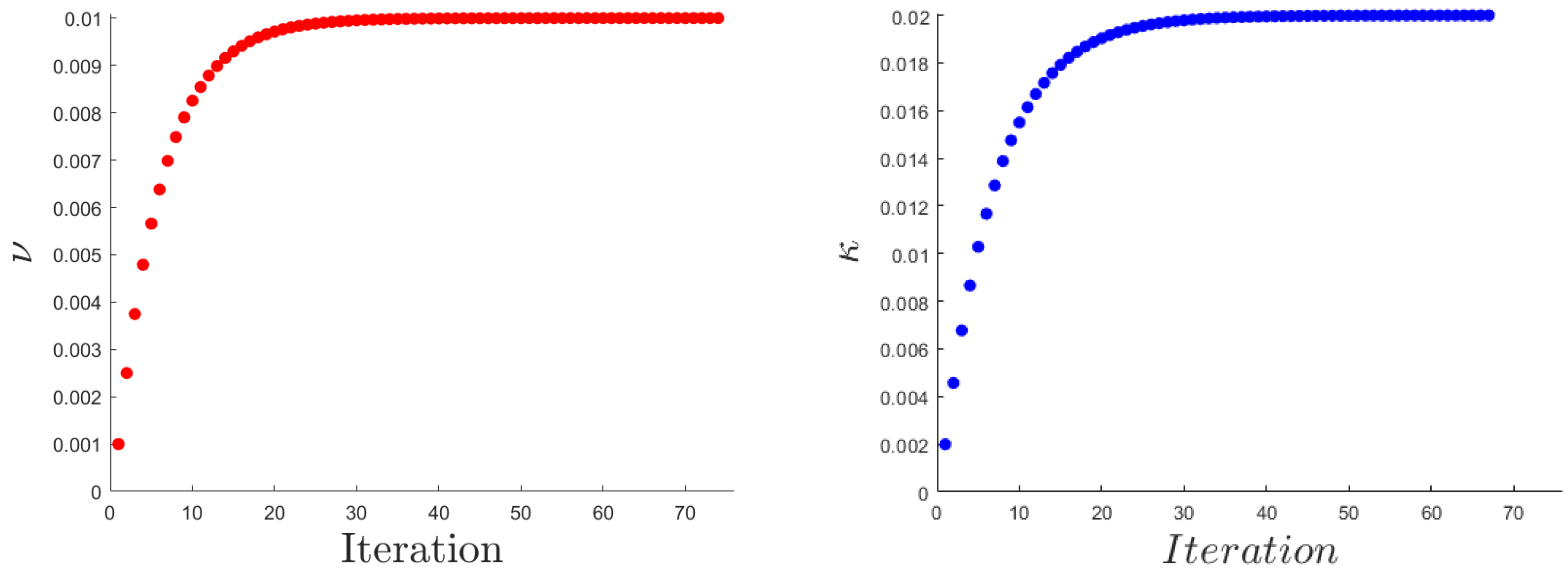
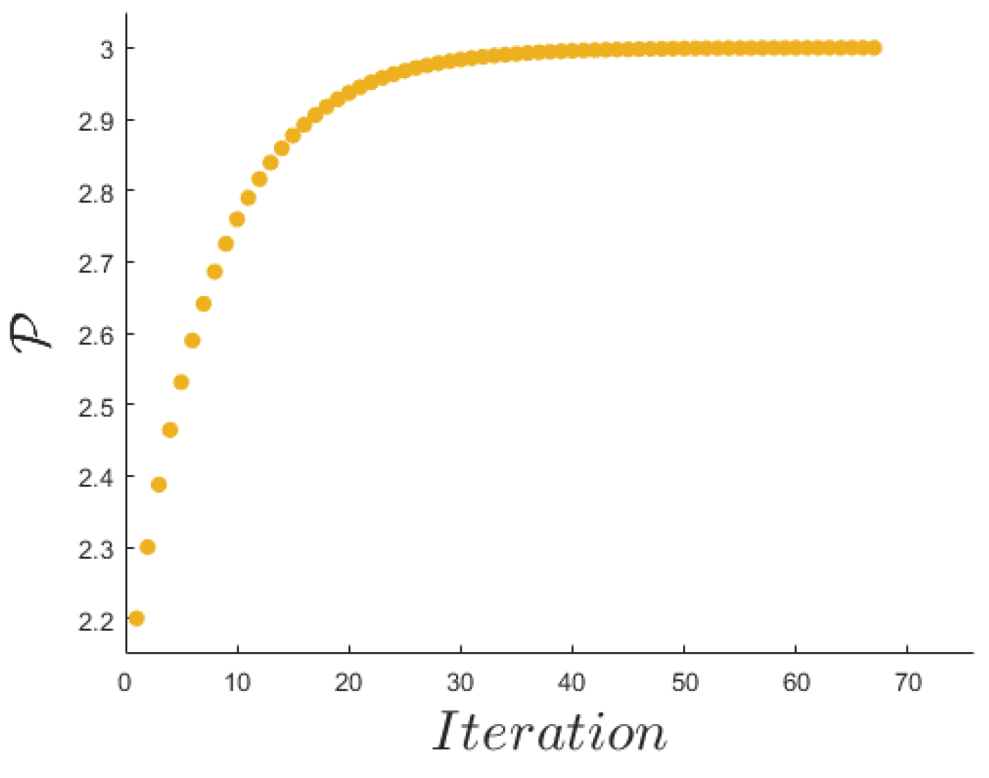
4.1. Validation Test

The initial data of the tumor cell parameter ${\phi }_0$ and the nutrient fraction ${\psi }_0$ are defined as

$$\begin{array}{c}{\phi }_0=-0.5\times e^{-x^2-y^2-z^2},\hfill \\ {\psi }_0=0.5\times e^{-x^2-y^2-z^2},\hfill \end{array}$$

where x, y, and z are the coordinates of the space meshing. The parameters $({\beta }_Q,{\beta }_{\mathsf{\Omega }})$, $(\epsilon ,\delta )$ and $({\beta }_{\nu },{\beta }_{\mathcal{P}},{\beta }_{\kappa })$ are set to

$$\begin{array}{cc}\hfill & {\beta }_{\nu }=0.3,{\beta }_{\mathcal{P}}=0.4,{\beta }_{\kappa }=0.35,\hfill \\ \hfill & \epsilon ={10}^{-6},\delta =0.8,\hfill \\ \hfill & {\beta }_{\mathsf{\Omega }}=0.25,{\beta }_Q=0.25.\hfill \end{array}$$

(24)

These particular choices are justified by a sensitivity analysis of the solutions with respect to the system’s parameters [21]. More specifically, the optimal regularization parameters in Tikhonov regularization are deduced according to the discrepancy principle based on an error estimators to control the convergence accuracy [24,25,26].

Figure 1, Figure 2, Figure 3, Figure 4, Figure 5 and Figure 6 show the evolution of the solutions $\phi$ and $\psi$ of the Cahn–Hilliard system at $\mathrm{T}=0,5,15,30,40$ and eventually 50, where it can be seen that the solution goes to a stationary point state which is in full alignment with the theoretical results (see also [1,2]). The optimal parameters that the algorithm converges to (associated to these figures) are

$$\begin{array}{c}\hfill \nu =0.0099591,\mathcal{P}=2.999607,\kappa =0.01995.\end{array}$$

The simulation shows that picking up large values of ${\beta }_{\nu }={\beta }_{\mathcal{P}}={\beta }_{\kappa }$ (in the simulation, these values were set as in (24)), and ${\beta }_{\mathsf{\Omega }}$ and ${\beta }_Q$ being set to $0.25$ leads to a rather fast convergence (algebraic) to the target parameters $({\nu }_d,{\mathcal{P}}_d,{\kappa }_d)$. However, we observed that picking up larger values for ${\beta }_{\mathsf{\Omega }}$ and ${\beta }_Q$, the algorithm we developed does not converge to the target values. We believe that a deeper numerical analysis of this algorithm is needed to provide a suitable range of the ”guess” parameters for the convergence to hold. Eventually, in the case of ${\nu }_d={\mathcal{P}}_d={\kappa }_d=0$, the algorithm is still converging, but by definition of the cost functional, toward the values set to have the solutions $({\phi }_{\mathsf{\Omega }},{\phi }_Q)$ with a suitable choice of the constants ${\beta }_{\mathsf{\Omega }}$ and ${\beta }_Q$.

Eventually, Figure 7 and Figure 8 show the evolution of the physical parameters in terms of the algorithm iterations. The initial parameters $\nu$ and $\kappa$ are chosen about ${10}^{-3}$ and $\mathcal{P}$ about $2.2$, and one can see (power type) convergence toward the target values

$$({\nu }_d,{\mathcal{P}}_d,{\kappa }_d)=(0.01,3,0.02).$$

4.2. Tumor Growth Computation

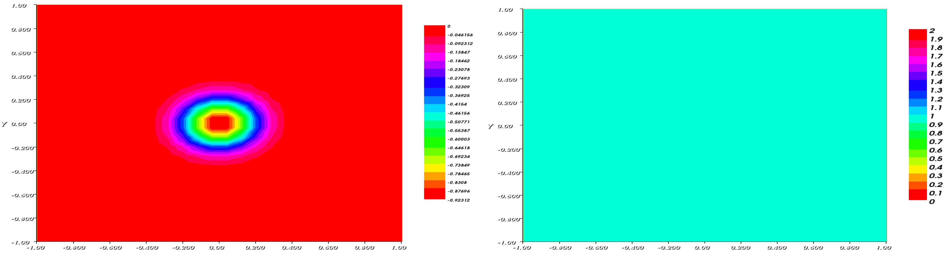
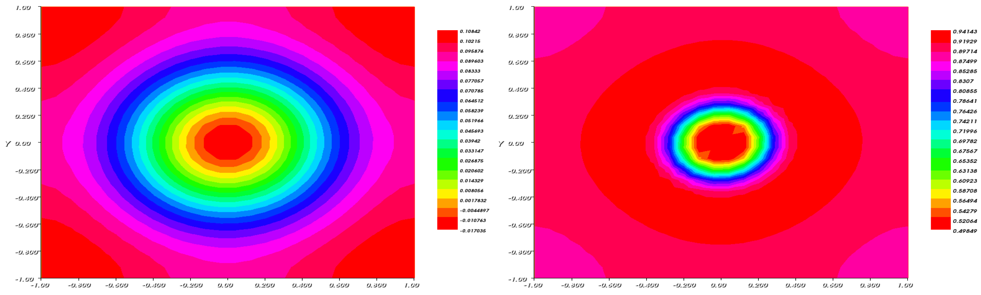
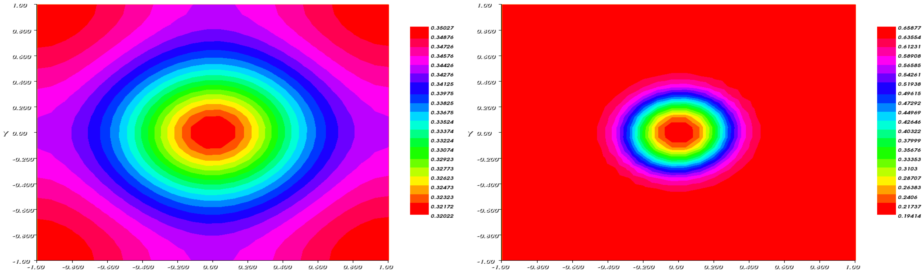
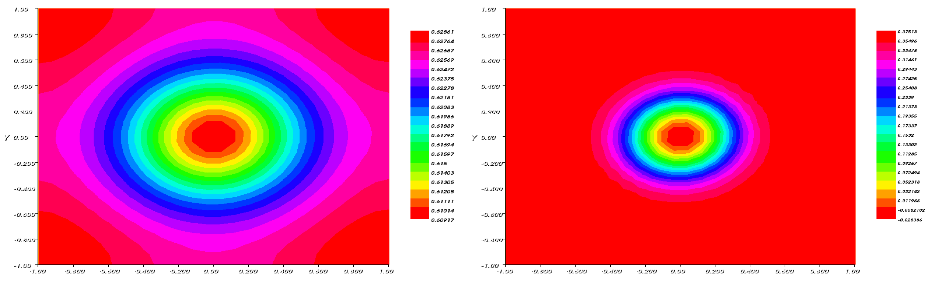
4.2.1. Two-Dimensional (2D) Case

In this section, we present a tumor growth example introduced in [3]. The simulation is performed based on the following data: the domain $\mathsf{\Omega }$ is considered as the square ${[-1,1]}^2$. The target parameters are set as $({\nu }_d,{\mathcal{P}}_d,{\kappa }_d)=(0.01,3,0.02)$. The initial data of the tumor cell parameter ${\phi }_0$ and the nutrient fraction ${\psi }_0$ are defined as

$$\begin{array}{c}{\phi }_0=-\left({\displaystyle \frac{1}{2.1}}{x}^2+{\displaystyle \frac{1}{1.9}}{y}^2\right)\in [-0.3,0.3],\hfill \\ {\psi }_0=1,\hfill \end{array}$$

where x and y are the coordinates of the space meshing. The parameters $({\beta }_{\mathsf{\Omega }},{\beta }_Q)$, $({\beta }_{\nu },{\beta }_{\mathcal{P}},{\beta }_{\kappa })$, and $(\epsilon ,\delta )$ are set to

$$\begin{array}{c}{\beta }_{\nu }=0.05,{\beta }_{\mathcal{P}}=0.025,{\beta }_{\kappa }=0.075,\hfill \\ {\beta }_{\mathsf{\Omega }}=0.2,{\beta }_Q=0.25,\hfill \\ \epsilon ={10}^{-6},\delta =0.8.\hfill \end{array}$$

Figure 9, Figure 10, Figure 11, Figure 12 and Figure 13 show the evolution of the solutions $\phi$ and $\psi$ of the Cahn–Hilliard system at $\mathrm{T}=0,5,15,30$ and eventually 50 related to the following optimal parameters

$$\begin{array}{c}\hfill \nu =0.009981,\mathcal{P}=2.998602,\kappa =0.019905.\end{array}$$

Note that the fraction $\psi$ describing the nutrient phase in the system is decreasing. This is justifying the nutrient consumption through the evolution of the tumor.

Figure 14 shows the total energy in the system. The total energy in system (1) decreases with respect to the evolution of time.

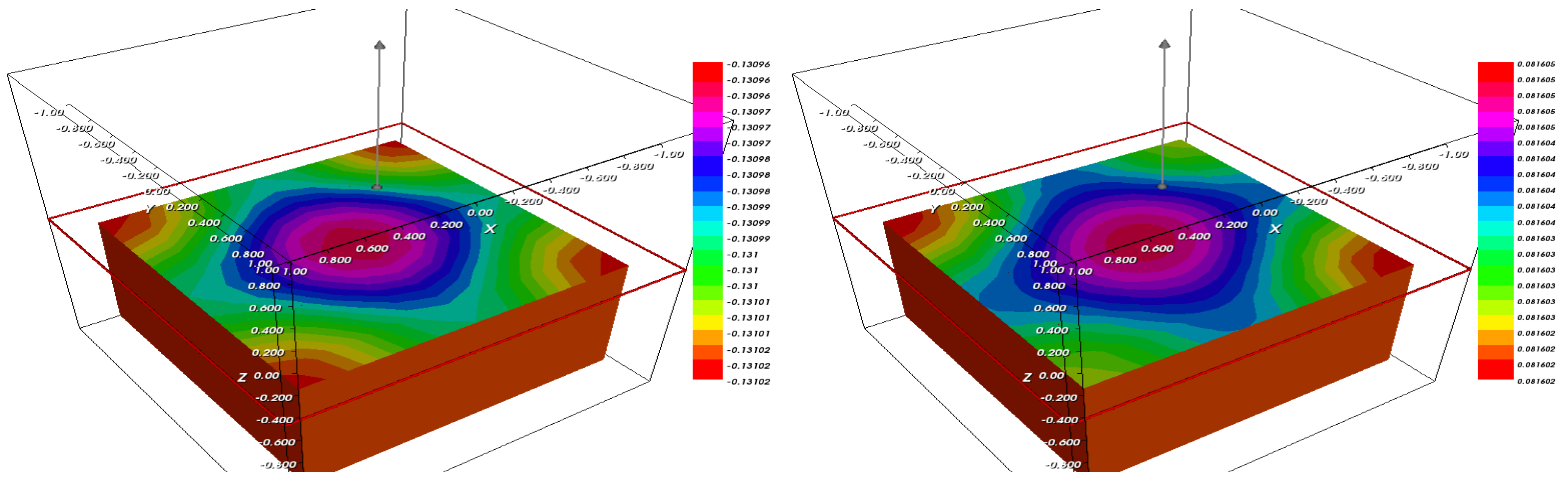
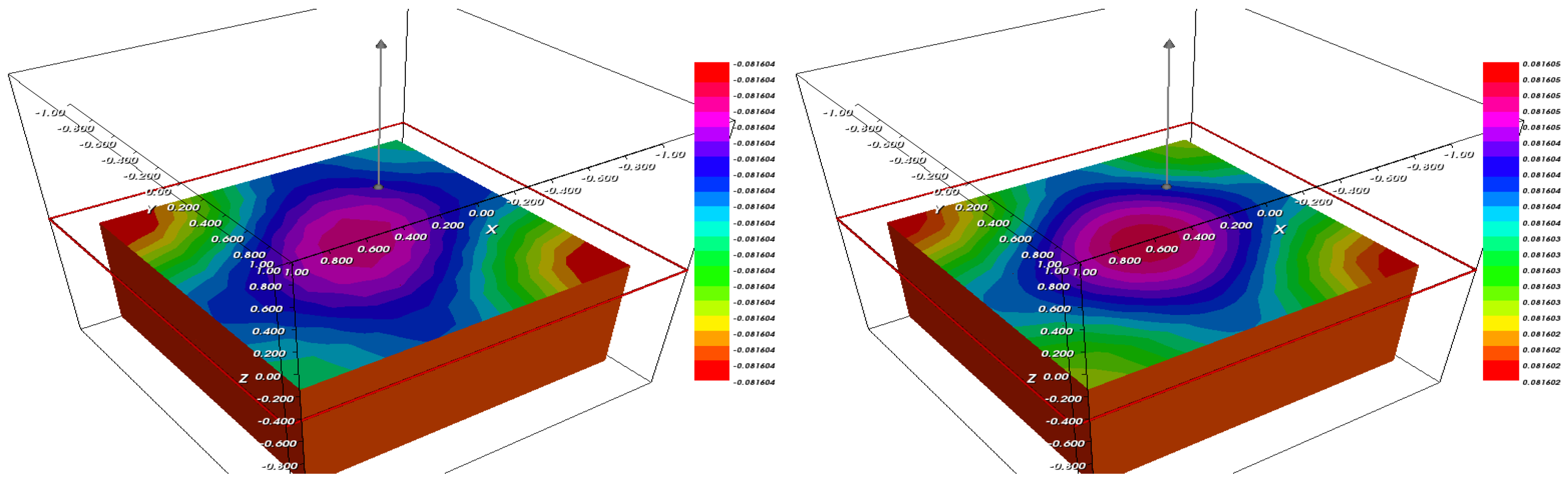
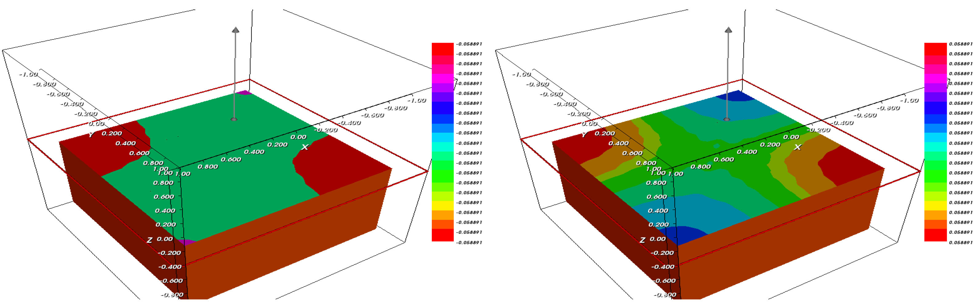
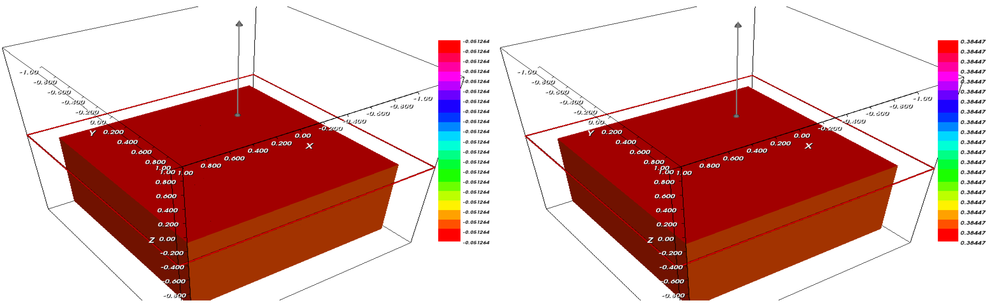
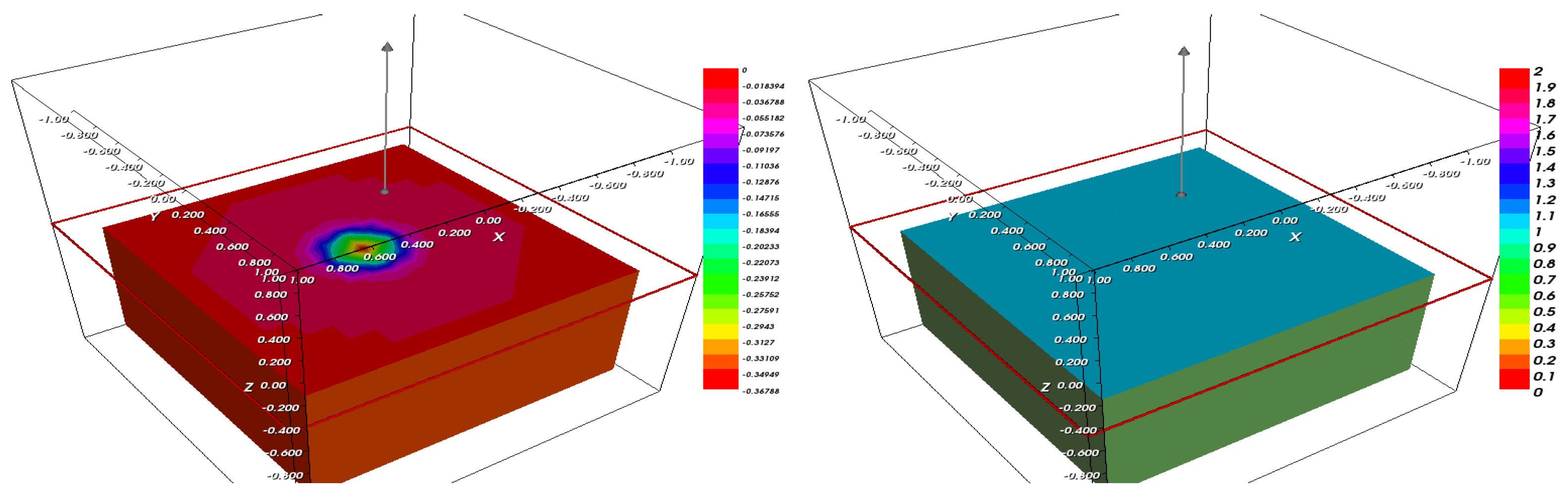
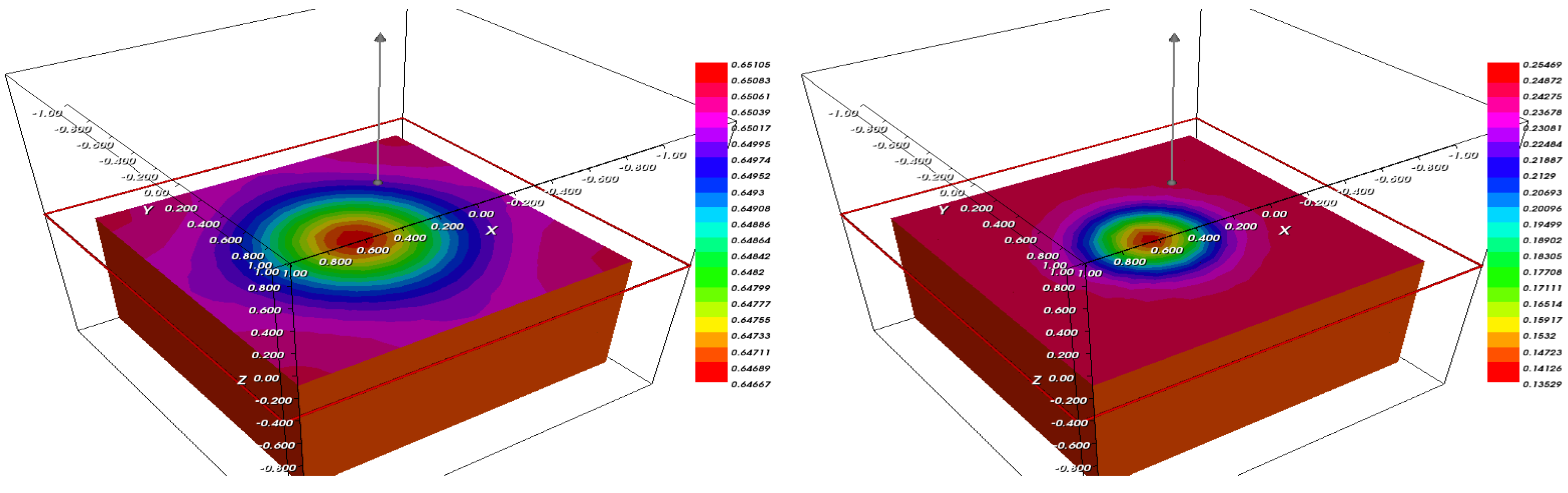
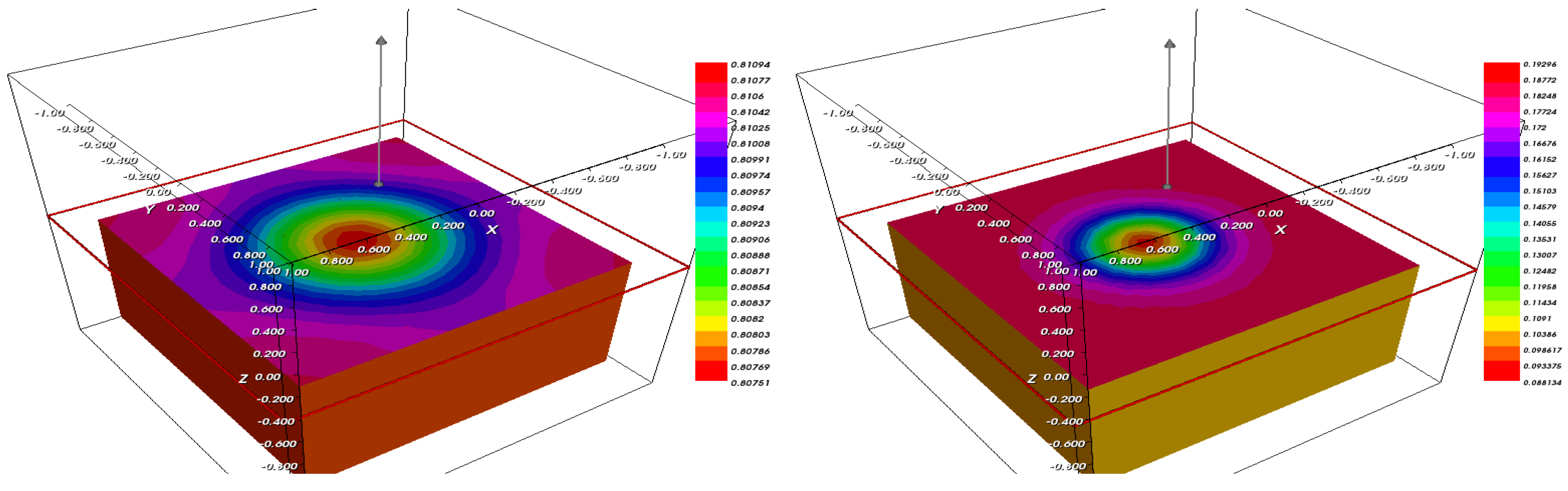
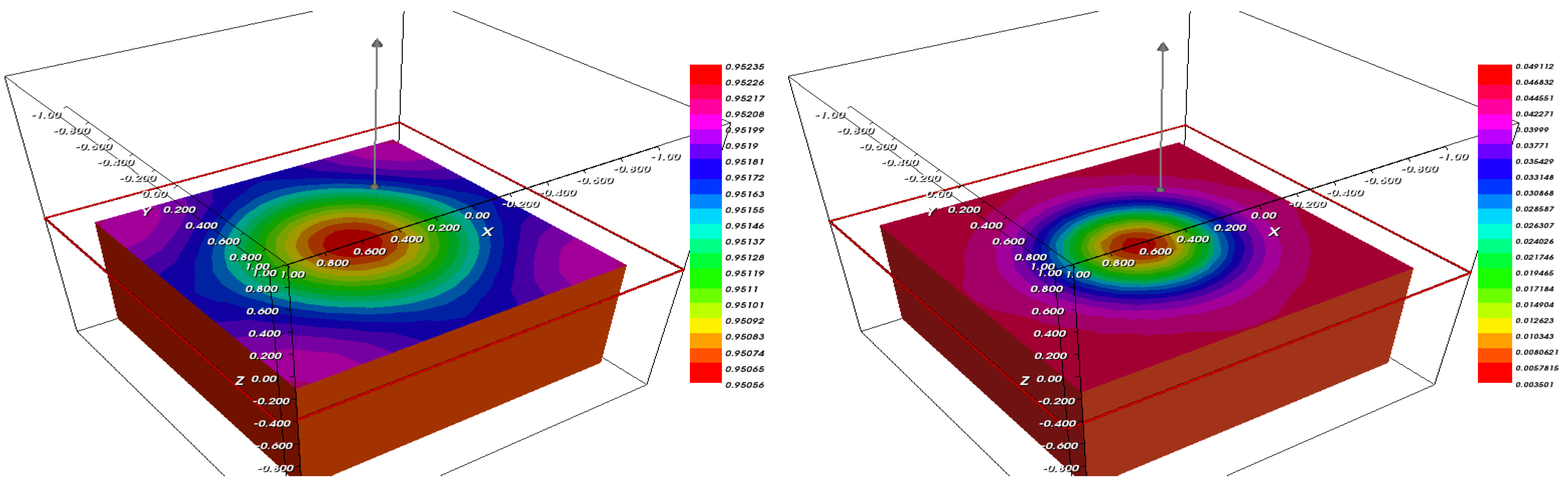
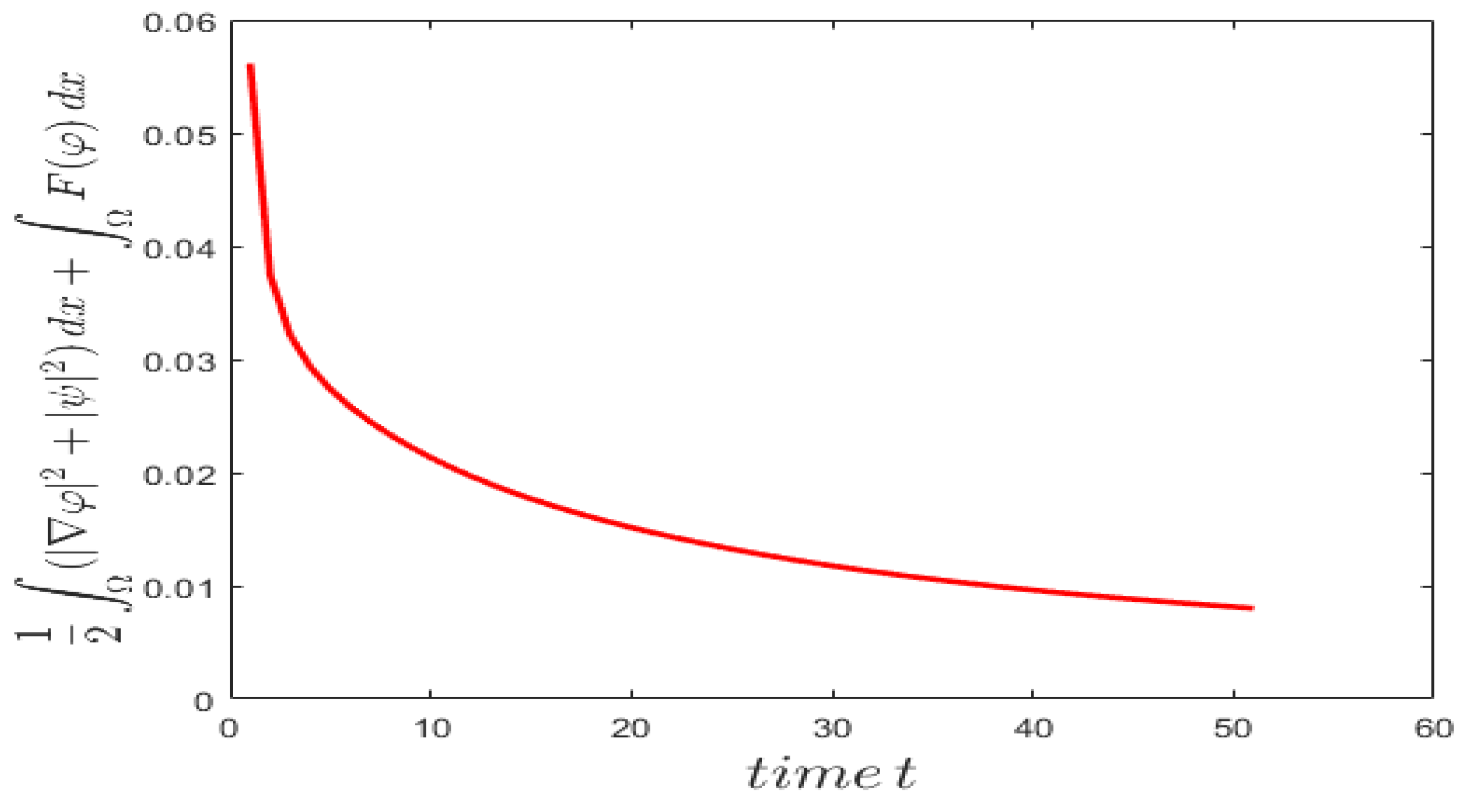
4.2.2. Three-Dimensional (3D) Case

In this section, we provide the $3D$ version of the previous example of tumor growth as defined in [3]. The simulation is carried out of the basis of the data below. The domain $\mathsf{\Omega }$ is considered as the cube ${[-1,1]}^3$. The initial data of the tumor cell parameter ${\phi }_0$ and the nutrient fraction ${\psi }_0$ are defined as

$$\begin{array}{c}{\phi }_0=-\left({\displaystyle \frac{1}{2.1}}{x}^2+{\displaystyle \frac{1}{1.9}}{y}^2+{\displaystyle \frac{1}{1.9}}{z}^2\right)\in [-0.3,0.3],\hfill \\ {\psi }_0=1,\hfill \end{array}$$

where x, y, and z are the coordinates of the space meshing. The parameters $(\delta ,\epsilon )$, $({\beta }_{\mathsf{\Omega }},{\beta }_Q)$, and $({\beta }_{\nu },{\beta }_{\mathcal{P}},{\beta }_{\kappa })$ are set to

$$\begin{array}{c}\hfill \begin{array}{c}{\beta }_{\nu }=0.05,{\beta }_{\mathcal{P}}=0.025,{\beta }_{\kappa }=0.075,\hfill \\ {\beta }_{\mathsf{\Omega }}=0.25,{\beta }_Q=0.25,\hfill \\ \epsilon ={10}^{-6},\delta =0.8.\hfill \end{array}\end{array}$$

Figure 15, Figure 16, Figure 17, Figure 18 and Figure 19 show the evolution of the tumor parameter $\phi$ and nutrient concentration $\psi$ solutions of the Cahn–Hilliard system (1) at times $\mathrm{T}=0,15,30,40$ and eventually 50. Note that the profile of the cell nutrient phase fraction is converted to tumor behavior at the end of the simulation. This explains the introduction of the proliferation function describing the evolution of the tumor by the consumption of nutrients.

Figure 15, Figure 16, Figure 17, Figure 18 and Figure 19 illustrate the profile of the solutions $\phi$ and $\psi$ of the Cahn–Hilliard system related to the following optimal parameters

$$\begin{array}{c}\hfill \nu =0.009901,\mathcal{P}=2.99892,\kappa =0.019987.\end{array}$$

We observe in Figure 20 that the total energy E defined in (3) of system (1) decreases in terms of time.

5. Conclusions

This paper is part of a series dedicated to the optimal control and data assimilation applied to tumor growth modeled by Cahn–Hilliard-type equations. In this contribution, we developed an optimal control theory coupled to the physical parameters identification process for the Cahn–Hilliard-type model (1). This was achieved by introducing and optimizing a cost function depending on both the functional solutions of system (1) and its physical parameters. This approach was inspired and motivated by the well-posedness results regarding system (1) in [1] and the sensitivity analysis results in [21]. We use a gradient descent method to solve the optimal problem (5). The derivation of the adjoint system allows us to express the gradient formula of the objective function in an easy way. Numerical computations show a fast convergence of the algorithm. The scheme is always stable with an appropriate CFL condition on the time step $\Delta t$ and mesh size h. The inclusion of the confidence region variation into the Newton–Gauss method ensures the convergence of the optimal problem in the ${\mathcal{U}}_{ad}$ admissible space. The numerical simulation is in full alignment with the theoretical results developed in this paper.

References

1. Frigeri, S.; Grasselli, M.; Rocca, E. On a diffuse interface model of tumour growth. Eur. J. Appl. Math. 2015, 26, 215–243. [Google Scholar] [CrossRef]
2. Garcke, H.; Yayla, S. Long-time dynamics for a Cahn–Hilliard tumor growth model with chemotaxis. Z. FüR Angew. Math. Und Phys. 2020, 71, 1–32. [Google Scholar] [CrossRef]
3. Hawkins-Daarud, A.; Van der Zee, K.G.; Oden, J.T. Numerical simulation of a thermodynamically consistent four-species tumor growth model. Int. J. Numer. Methods Biomed. Eng. 2012, 28, 3–24. [Google Scholar] [CrossRef] [PubMed]
4. Miranville, A. The Cahn–Hilliard equation: Recent advances and applications. Soc. Ind. Appl. Math. 2019, 123, 57–62. [Google Scholar]
5. Araujo, R.P.; McElwain, D.S. A history of the study of solid tumour growth: The contribution of mathematical modelling. Bull. Math. Biol. 2004, 66, 1039–1091. [Google Scholar] [CrossRef]
6. Cristini, V.; Lowengrub, J. Multiscale Modeling of Cancer: An Integrated Experimental and Mathematical Modeling Approach; Cambridge University Press: Cambridge, UK, 2010. [Google Scholar]
7. Garcke, H.; Trautwein, D. Numerical analysis for a Cahn–Hilliard system modeling tumour growth with chemotaxis and active transport. J. Numer. Math. 2022, 30, 295–324. [Google Scholar] [CrossRef]
8. Knopf, P.; Signori, A. Existence of weak solutions to multiphase Cahn–Hilliard–Darcy and Cahn–Hilliard–Brinkman models for stratified tumor growth with chemotaxis and general source terms. Commun. Partial. Differ. Equations 2022, 47, 233–278. [Google Scholar] [CrossRef]
9. Lowengrub, J.S.; Frieboes, H.B.; Jin, F.; Chuang, Y.L.; Li, X.; Macklin, P.; Wise, S.M.; Cristini, V. Nonlinear modelling of cancer: Bridging the gap between cells and tumours. Nonlinearity 2009, 23, R1. [Google Scholar] [CrossRef] [Green Version]
10. Oden, J.T.; Prudencio, E.E.; Hawkins-Daarud, A. Selection and assessment of phenomenological models of tumor growth. Math. Model. Methods Appl. Sci. 2013, 23, 1309–1338. [Google Scholar] [CrossRef]
11. Rocca, E.; Schimperna, G.; Signori, A. On a Cahn–Hilliard–Keller–Segel model with generalized logistic source describing tumor growth. J. Differ. Equations 2023, 343, 530–578. [Google Scholar] [CrossRef]
12. Storvik, E.; Both, J.W.; Nordbotten, J.M.; Radu, F.A. A Cahn–Hilliard–Biot system and its generalized gradient flow structure. Appl. Math. Lett. 2022, 126, 107799. [Google Scholar] [CrossRef]
13. Cristini, V.; Li, X.; Lowengrub, J.S.; Wise, S.M. Nonlinear simulations of solid tumor growth using a mixture model: Invasion and branching. J. Math. Biol. 2009, 58, 723–763. [Google Scholar] [CrossRef] [PubMed] [Green Version]
14. Oden, J.T.; Hawkins, A.; Prudhomme, S. General diffuse-interface theories and an approach to predictive tumor growth modeling. Math. Model. Methods Appl. Sci. 2010, 20, 477–517. [Google Scholar] [CrossRef] [Green Version]
15. Chatelain, C.; Balois, T.; Ciarletta, P.; Amar, M.B. Emergence of microstructural patterns in skin cancer: A phase separation analysis in a binary mixture. New J. Phys. 2011, 13, 115013. [Google Scholar] [CrossRef]
16. Frieboes, H.B.; Jin, F.; Chuang, Y.L.; Wise, S.M.; Lowengrub, J.S.; Cristini, V. Three-dimensional multispecies nonlinear tumor growth—II: Tumor invasion and angiogenesis. J. Theor. Biol. 2010, 264, 1254–1278. [Google Scholar] [CrossRef] [Green Version]
17. Hawkins-Daarud, A.; Prudhomme, S.; van der Zee, K.G.; Oden, J.T. Bayesian calibration, validation, and uncertainty quantification of diffuse interface models of tumor growth. J. Math. Biol. 2013, 67, 1457–1485. [Google Scholar] [CrossRef]
18. Garcke, H.; Lam, K.F. Analysis of a Cahn-Hilliard system with non-zero Dirichlet conditions modeling tumor growth with chemotaxis. Discret. Contin. Dyn. Syst. 2017, 37, 4277–4308. [Google Scholar] [CrossRef] [Green Version]
19. Garcke, H.; Lam, K.F. Well-posedness of a Cahn–Hilliard system modeling tumour growth with chemotaxis and active transport. Eur. J. Appl. Math. 2017, 28, 284–316. [Google Scholar] [CrossRef] [Green Version]
20. Garcke, H.; Lam, K.F.; Sitka, E.; Styles, V. A Cahn–Hilliard–Darcy model for tumour growth with chemotaxis and active transport. Math. Model. Methods Appl. Sci. 2016, 26, 1095–1148. [Google Scholar] [CrossRef]
21. Kadiri, M.; Trabelsi, S. Cahn-Hilliard equation: Continuous dependence on physical parameters and sensitivity analysis. 2022; submitted. [Google Scholar]
22. Kadiri, M.; Titi, E.S.; Trabelsi, S. Data assimilation for a Cahn-hilliard equations modeling tumour growth. 2022; submitted. [Google Scholar]
23. Kaltenbacher, B. Some Newton-type methods for the regularization of nonlinear ill-posed problems. Inverse Probl. 1997, 13, 729–753. [Google Scholar] [CrossRef]
24. Gazzola, S.; Reichel, L. A new framework formulti-parameter regularization. Bit Numer. Math. 2016, 56, 919–949. [Google Scholar] [CrossRef]
25. Hansen, P.C. The L-Curve and Its Use in the Numerical Treatment of Inverse Problems; Computational Inverse Problems in Electro Cardiology; WIT Press: Southampton, UK, 1999; pp. 119–142. [Google Scholar]
26. Kaltenbacher, B.; Kirchner, A.; Vexler, B. Adaptive discretizations for the choice of a Tikhonov regularization parameter in nonlinear inverse problems. Inverse Problems 2011, 27, 125008. [Google Scholar] [CrossRef]
Figure 1. The fraction φ (left), and ψ (right) after T = 0 .
Mathematics 11 01607 g001
Figure 2. The fraction φ (left) and ψ (right) after T = 5 .
Mathematics 11 01607 g002
Figure 3. The fraction φ (left) and ψ (right) after T = 15 .
Mathematics 11 01607 g003
Figure 4. The fraction φ (left) and ψ (right) after T = 30 .
Mathematics 11 01607 g004
Figure 5. The fraction φ (left) and ψ (right) after T = 40 .
Mathematics 11 01607 g005
Figure 6. The fraction φ (left) and ψ (right) after T = 50 .
Mathematics 11 01607 g006
Figure 7. The variation of the viscosity ν (left) and κ (right) in terms of algorithm iterations.
Mathematics 11 01607 g007
Figure 8. The proliferation rate P in terms of algorithm iterations.
Mathematics 11 01607 g008
Figure 9. The fraction φ (left) and ψ (right) after T = 0 .
Mathematics 11 01607 g009
Figure 10. The fraction φ (left) and ψ (right) after T = 5 .
Mathematics 11 01607 g010
Figure 11. The fraction φ (left) and ψ (right) after T = 15 .
Mathematics 11 01607 g011
Figure 12. The fraction φ (left) and ψ (right) after T = 30 .
Mathematics 11 01607 g012
Figure 13. The fraction φ (left) and ψ (right) after T = 50 .
Mathematics 11 01607 g013
Figure 14. The total energy defined in ( 3 ) of the system.
Mathematics 11 01607 g014
Figure 15. The fraction φ (left) and ψ (right) after T = 0 .
Mathematics 11 01607 g015
Figure 16. The fraction φ (left) and ψ (right) after T = 15 .
Mathematics 11 01607 g016
Figure 17. The fraction φ (left) and ψ (right) after T = 30 .
Mathematics 11 01607 g017
Figure 18. The fraction φ (left) and ψ (right) after T = 40 .
Mathematics 11 01607 g018
Figure 19. The fraction φ (left) and ψ (right) after T = 50 .
Mathematics 11 01607 g019
Figure 20. The total energy defined in (3) of the system.
Mathematics 11 01607 g020
Disclaimer/Publisher’s Note: The statements, opinions and data contained in all publications are solely those of the individual author(s) and contributor(s) and not of MDPI and/or the editor(s). MDPI and/or the editor(s) disclaim responsibility for any injury to people or property resulting from any ideas, methods, instructions or products referred to in the content.