Cumulant-Based Goodness-of-Fit Tests for the Tweedie, Bar-Lev and Enis Class of Distributions

Abstract

The class of natural exponential families (NEFs) of distributions having power variance functions (NEF-PVFs) is huge (uncountable), with enormous applications in various fields. Based on a characterization property that holds for the cumulants of the members of this class, we developed a novel goodness-of-fit (gof) test for testing whether a given random sample fits fixed members of this class. We derived the asymptotic null distribution of the test statistic and developed an appropriate bootstrap scheme. As the content of the paper is mainly theoretical, we exemplify its applicability to only a few elements of the NEF-PVF class, specifically, the gamma and modified Bessel-type NEFs. A Monte Carlo study was executed for examining the performance of both—the asymptotic test and the bootstrap counterpart—in controlling the type I error rate and evaluating their power performance in the special case of gamma, while real data examples demonstrate the applicability of the gof test to the modified Bessel distribution.

1. Introduction

Let $\mathbf{\nu }$ be a positive Radon measure on $\mathbb{R}$, $\mathcal{L}\left(\theta \right)={\int }_{\mathbb{R}}{\mathrm{E}}^{\theta x}d\mathbf{\nu }\left(x\right)$ be its Laplace transform and $D=\left\{\theta \in \mathbb{R}:\mathcal{L}\left(\theta \right)<\infty \right\}$ be its effective domain. Let us assume that $\Theta \doteq in\mathrm{T}D\ne \varnothing$; then, the natural exponential family (NEF) generated by $\mathbf{\nu }$ is the set $\mathcal{F}=\{F_{\theta }:\theta \in \Theta \subset R\}$ of probability distributions defined by

$$d{F}_{\theta }\left(x\right)=exp\{\theta x+c\left(\theta \right)\}dv\left(x\right),\theta \in \Theta \subset R,$$

(1)

where $c\left(\theta \right)$ is real, analytic and strictly concave on $\Theta$; and $k_j\left(\theta \right)=-\frac{d^{j}c\left(\theta \right)}{d{\theta }^j}$, $j\in \mathbb{N}$, is the j-th cumulant of $F_{\theta }$. In particular, the mean and variance of $F_{\theta }$ are given by $\mu =\mu \left(\theta \right)=k_1\left(\theta \right)$ and ${\sigma }^2={\sigma }^2\left(\theta \right)=k_2\left(\theta \right)$, respectively. As $c\left(\theta \right)$ is strictly concave on $\Theta$, the mean domain $\Omega =\mu (\mathrm{i}\mathrm{n}\mathrm{t}\Theta )$ of $\mathcal{F}$ is an open interval; inverse map $\theta ⟼\mu \left(\theta \right)$ is one to one; and its inverse function $\psi :\Omega ⟶\Theta$ is well defined. Let us denote $V\left(\mu \right)={\sigma }^2\left(\psi \left(\mu \right)\right)$; then, the pair $(V,\Omega )$ is called the variance function (VF) of $\mathcal{F}$. The VF uniquely determines $\mathcal{F}$ within the class of NEFs (see an appropriate survey in [1]).

An NEF $\mathcal{F}$ is said to have a power variance function (hereafter, NEF-PVF) if V has the form of $V\left(\mu \right)=a{\mu }^{\gamma }$, $\mu \in \Omega$, for some constants $a>0$ and power parameter $\gamma \in \mathbb{R}$. The class of NEF-PVFs has been introduced independently and in different contexts by [2,3,4]. In this context, comprehensive details can be found in [5]. Despite the fact that all of the NEF-PVFs are often referred to as Tweedie class, for the reasons explained in [5] (and already adopted in [6,7]), we shall henceforth call them the Tweedie, Bar-Lev and Enis models and use the notation $X\sim {\mathrm{T}\mathrm{B}\mathrm{E}}_{\gamma }(\mu ,a)$ to indicate that random variable X has a distribution that belongs to the ${\mathrm{T}\mathrm{B}\mathrm{E}}_{\gamma }(\mu ,a)$ model with mean $\mu$, scale parameter a and power parameter $\gamma$. Finally, argument $(\mu ,a)$ will be skipped when unnecessary, and we will write ${\mathrm{T}\mathrm{B}\mathrm{E}}_{\gamma }$.

${\mathrm{T}\mathrm{B}\mathrm{E}}_{\gamma }$ models constitute a huge (uncountable) class, as for each power parameter, $\gamma \in \mathbb{R}∕(0,1)$, there corresponds a natural exponential family member, while for $\gamma \in (0,1)$, no NEF exists. Depending on the value of power parameter $\gamma$, NEF-PVFs include, as special cases (see for instance [8]), normal ($\gamma =0$), Poisson-type ($\gamma =1$) and gamma ($\gamma =2$) NEFs; the family of compound Poisson distributions generated by gamma variates ($1<\gamma <2$); NEFs generated by positive stable distributions with stable index in $\left(0,1\right)$ and supported on ${\mathbb{R}}^{+}$ ($\gamma >2$); and NEFs generated by extreme stable distributions with stable index in $(1,2)$ and supported on $\mathbb{R}$ ($\gamma <0$). Among the NEFs with $\gamma >2$, we find the inverse Gaussian ($\gamma =3$), modified Bessel-type ($\gamma =2.5$) and Whittaker-type ($\gamma =4$) distributions.

Since ${\mathrm{T}\mathrm{B}\mathrm{E}}_{\gamma }$ models have been utilized in various fields, such as actuarial studies, assay analysis, survival analysis, time spent splicing telephone cables, ecology and meteorology (see [9,10] and the references cited therein), it is important to test the hypothesis that a given sample stems from a ${\mathrm{T}\mathrm{B}\mathrm{E}}_{\gamma }$ model with some $\gamma$.

In this paper, we propose a novel goodness-of-fit (gof) test for ${\mathrm{T}\mathrm{B}\mathrm{E}}_{\gamma }$ distributions for any fixed power parameter $\gamma \in \mathbb{R}∕[0,1)$. The test is based on a cumulant-based relationship existing among all members of ${\mathrm{T}\mathrm{B}\mathrm{E}}_{\gamma }$ models, for $\gamma \in \mathbb{R}∕[0,1)$. These cumulant-based relationships were obtained by [11,12] as a characterization of any member of the ${\mathrm{T}\mathrm{B}\mathrm{E}}_{\gamma }$ class with $\gamma \in \mathbb{R}∕[0,1)$. To the best of our knowledge, this is the first attempt to utilize these characterization properties for developing gof tests that hold for all members of ${\mathrm{T}\mathrm{B}\mathrm{E}}_{\gamma }$ with $\gamma \in \mathbb{R}∕[0,1)$. Admittedly, a large number of tests have been proposed for ${\mathrm{T}\mathrm{B}\mathrm{E}}_0$ (normal), ${\mathrm{T}\mathrm{B}\mathrm{E}}_1$ (Poisson), ${\mathrm{T}\mathrm{B}\mathrm{E}}_2$ (gamma) and ${\mathrm{T}\mathrm{B}\mathrm{E}}_3$ (inverse Gaussian). On the other hand, we do not know of any test for ${\mathrm{T}\mathrm{B}\mathrm{E}}_{\gamma }$, where $\gamma <0$ and $\gamma >2$ (except for $\gamma =3)$. The latter ${\mathrm{T}\mathrm{B}\mathrm{E}}_{\gamma }$ are generated by either extreme stable distributions ($\gamma <0$) and are supported on $\mathbb{R}$ or positive stable distributions ($\gamma >2$) and are supported on ${\mathbb{R}}^{+}$. In both cases, the respective densities are unimodal, leptokurtic and absolutely continuous with respect to the Lebesgue measure. Therefore, they are suitable candidates for modeling continuous data. Unlike the normal, gamma and inverse Gaussian NEFs, however, these stable densities cannot be expressed in terms of elementary functions but rather in terms of series expansion. For instance, for any fixed $\gamma >2$, the corresponding density of the corresponding ${\mathrm{T}\mathrm{B}\mathrm{E}}_{\gamma }$ model is given by (see [3])      

$$\begin{array}{c}\hfill d{F}_{\theta }\left(x\right)=\left\{-\frac{1}{\pi }\sum _{k=0}^{\infty }\frac{{(-1)}^k}{k!}sin\left(\pi \rho k\right)\frac{{(1-\rho )}^{k(1-\rho )}\Gamma (\rho k+1)}{{\rho }^k{a}^{k(1-\rho )}{x}^{\rho k+1}}\right\}\\ \\ \hfill \times exp\left\{\theta x+\frac{1-\rho }{a\rho }{\left[\frac{a\theta }{\rho -1}\right]}^{\rho }\right\}dx,x>0,\theta <0,0<\rho \doteq \frac{2-\gamma }{1-\gamma }<1.\end{array}$$

(2)

For some rational values of $\rho \in (0,1)$ (or $\gamma \in (2,\infty )$) the corresponding densities in (2) can be expressed in terms of transcendental functions, e.g., the modified Bessel distribution ($\rho =1/3$ or $\gamma =2.5$) and the Whittaker-type distribution ($\rho =2/3$ or $\gamma =4$). Series expansions similar to (2) are also available for stable densities of ${\mathrm{T}\mathrm{B}\mathrm{E}}_{\gamma }$ with $\rho \in (1,2)$ (or $\gamma \in (-\infty ,0)$), which are supported on $\mathbb{R}$. The complexity of the series expansion form of the ${\mathrm{T}\mathrm{B}\mathrm{E}}_{\gamma }$ models generated by stable densities could be the reason why these have not been used for any statistical modeling purposes. Fortunately, nowadays, the availability of powerful software allows the cumbersome calculations of various functionals related to these densities to be conducted. Indeed, our proposed gof test for TBE models might be an important step for employing them in the statistical modeling and analysis of continuous sets of data.

The paper is organized as follows: Section 2 presents the cumulant-based relationships existing among ${\mathrm{T}\mathrm{B}\mathrm{E}}_{\gamma }$ models, for $\gamma \in \mathbb{R}∕[0,1)$, and also some basic tools needed for constructing the proposed gof test. It should be noted that for any fixed permissible power parameter $\gamma$, the cumulant relation that we use for constructing our proposed gof tests characterizes the corresponding ${\mathrm{T}\mathrm{B}\mathrm{E}}_{\gamma }$ model. Section 3 introduces the proposed gof test. In particular, it presents the test statistic, its asymptotic null distribution and a bootstrap approximation. As the goal of the paper is mainly theoretical, i.e., introducing gof tests for all ${\mathrm{T}\mathrm{B}\mathrm{E}}_{\gamma }$ models with $\gamma \in \mathbb{R}∕[0,1)$, we exemplify its applicability to only two models of the TBE class. These two models are the gamma and modified Bessel NEFs. Specifically, Section 4.1 exemplifies its applicability to the gamma NEF with respect to various alternatives and existing tests. The performance of the gof test is investigated with a simulation study. In particular, its performance in terms of controlling the type I error rate is examined, while its power performance is also evaluated. In Section 4.2, we demonstrate its applicability to the modified Bessel NEF, and we investigate the nominal level attainment and compute the respective p-values for two real data sets. Obviously, similar applications can be executed for all other ${\mathrm{T}\mathrm{B}\mathrm{E}}_{\gamma }$ models with $\gamma >2$ or $\gamma <0$. Concluding remarks and some open problems are introduced in Section 5. All proofs of statements (theorems and corollaries) in this paper are relegated to Appendix A.

In the sequel, we use the following notation: Let $\mathbf{X}=(X_1,...,X_n)$ be a random sample of size n taken from a population with distribution F, where $X_1$,...,$X_n$ are i.i.d.; let ${\overline{X}}_n$ be the sample mean and $L_j={\sum }_{i=1}^n{X}_i^j$, $j\in \mathbb{N}$. We also denote, with $k_i$, the i−th cumulant, $i=1,2,...,$ associated with F. Let us recall that cumulant $k_i$ can be obtained by differentiating the cumulant-generating function $K\left(t\right)=logE\left(e^{tX}\right)$i times and evaluating the result at zero.

2. TBE Cumulant Relationships among ${\mathrm{T}\mathrm{B}\mathrm{E}}_{\gamma }$ Models and Some Testing Tools

A common approach to constructing gof tests is to utilize a characterization of the members of the family of distributions being considered. In this frame, the members of the ${\mathrm{T}\mathrm{B}\mathrm{E}}_{\gamma }$ models satisfy the following propositions, some of which characterize these models (see [11,12]). The proof of Proposition 1 can be found in [11] for $\gamma \ge 1$ and in Section 3 of [12] for $\gamma <0$. The proof of Proposition 2 can be conducted by utilizing tools available in [11,12,13]. We omit the proof of Proposition 2, as it is long and entirely not essential for the development of the results of this paper.

Proposition 1.

If X$\sim {TBE}_{\gamma }$, with $\gamma \in \mathbb{R}∕[0,1)$, then

$$S_r\left(\gamma \right)\doteq k_{r+2}{k}_r-{\beta }_r\left(\gamma \right)k_{r+1}^2=0,r\in \mathbb{N},$$

(3)

where $k_j$ is the j-th cumulant of the corresponding ${TBE}_{\gamma }$ and

$${\beta }_r\left(\gamma \right)=\frac{r\gamma -(r-1)}{(r-1)\gamma -(r-2)}.$$

(4)

Proposition 2.

Let us assume that X is an r.v. of a distribution in the NEF class of distributions. Then, for any $\gamma \in \mathbb{R}∕[0,1)$, property (3) in Proposition 1 holds if and only if $X\sim {TBE}_{\gamma }$.

Remark 1.

Note that $\gamma =0$, representing the normal distribution, is excluded from the statement of Proposition 1 as it does not satisfy relation (3). Other cumulant-based relations hold for the normal NEF as $k_p{k}_q=0$, where $q,p\in \mathbb{N}$; $q\le p$; and $p\ge 3$. Accordingly, our gof test does not hold for the normal NEF.

Proposition 1 implies that if relation (3) does not hold for $\gamma ={\gamma }_0$, then the sample is not taken from ${\mathrm{T}\mathrm{B}\mathrm{E}}_{{\gamma }_0}$. For instance, for the gamma distribution with shape parameter $\alpha$ and rate parameter $\beta$, the first three cumulants are given by

$$k_1=\alpha /\beta ,k_2=\alpha /{\beta }^2,k_3=2\alpha /{\beta }^3,$$

which results in

$$S_1\left(\gamma \right)=k_3{k}_1-\gamma k_2^2=(2-\gamma )\frac{{\alpha }^2}{{\beta }^4}.$$

(5)

Thus, $S_1\left(\gamma \right)$ is equal to 0 if and only if $\gamma =2$. Moreover, for the inverse Gaussian distribution with mean $\mu$ and shape parameter $\lambda$, one has

$$k_1=\mu ,k_2={\mu }^3/\lambda ,k_3=3{\mu }^5/{\lambda }^2,$$

and thus

$$S_1\left(\gamma \right)=k_3{k}_1-\gamma k_2^2=\frac{(3-\gamma ){\mu }^6}{{\lambda }^2}.$$

(6)

Thus, $S_1\left(\gamma \right)=0$ if and only if $\gamma =3$. Finally, for the Poisson distribution with parameter $\lambda$, since $k_1=k_2=k_3=\lambda$, we have

$$S_1\left(\gamma \right)=k_3{k}_1-\gamma k_2^2=(1-\gamma ){\lambda }^2.$$

(7)

Thus, $S_1\left(\gamma \right)=0$ if and only if $\gamma =1$.

The reverse statement is obviously incorrect if F is not an NEF, i.e., there exist distributions F not in the NEF class for which $S_1\left(\gamma \right)=0$. For instance, let us consider F to be a lognormal distribution $LN(\mu ,\sigma )$ with p.d.f. of the form

$$f(x;\mu ,\sigma )=exp\left(-{(ln\left(x\right)-\mu )}^2/\left(2{\sigma }^2\right)\right)/\left(\sigma x\sqrt{2\pi }\right),\sigma >0,x>0.$$

Then (see [14]),

$$k_1=exp\left(\mu \right)exp({\sigma }^2/2),k_2=exp\left(2\mu \right)exp\left({\sigma }^2\right)\left(exp\left({\sigma }^2\right)-1\right)$$

and

$$k_3=exp\left(3\mu \right)exp(3{\sigma }^2/2){\left(exp\left({\sigma }^2\right)-1\right)}^2\left(exp\left({\sigma }^2\right)+2\right),$$

in which case,

$$S_1\left(\gamma \right)=exp\left(4\mu \right)exp\left(2{\sigma }^2\right){\left(exp\left({\sigma }^2\right)-1\right)}^2\left(exp\left({\sigma }^2\right)+2-\gamma \right).$$

(8)

Therefore, $S_1\left(\gamma \right)=0$ if $\gamma =e^{{\sigma }^2}+2$. A special case of this situation is when $F\sim LN(\mu ,\sqrt{ln\left(2\right)})$. Then, $S_1\left(4\right)=0$, while the lognormal family is not an NEF (note that $S_1\left(4\right)=0$ holds for Whittaker-type NEFs). This example illustrates that if F is not an NEF; then, the relationship $S_1\left(\gamma \right)=0$ does not characterize the distribution involved.

As relation (3), $r\in \mathbb{N}$, characterizes an NEF within the class of NEFs, a test for a null hypothesis in which $F\sim$${\mathrm{T}\mathrm{B}\mathrm{E}}_{\gamma }$ against a general alternative can be based on any estimator of $S_r\left(\gamma \right)$, $r\in \mathbb{N}$. Nonetheless, as an unbiased estimator of $S_r\left(\gamma \right),r>1,$ has a cumbersome form, we shall restrict our study to the case $r=1$. For ease of notation, we shall henceforth denote $S_1\left(\gamma \right)$ with $S\left(\gamma \right)$ and its unbiased estimator with $\widehat{S}\left(\gamma \right)$.

Indeed, an unbiased estimator $\widehat{S}\left(\gamma \right)$ of $S\left(\gamma \right)=k_3{k}_1-\gamma k_2^2$ has the following polynomial structure (see [11]):

$$\widehat{S}\left(\gamma \right)={\widehat{T}}_{1,3}-\gamma {\widehat{T}}_{2,2},\gamma \in \mathbb{R}∕[0,1),$$

(9)

where

$${\widehat{T}}_{1,3}=\frac{1}{n_{\left(2\right)}}\sum _{j\ne k}{X}_j^3{X}_k-\frac{3}{n_{\left(3\right)}}\sum _{j\ne k\ne l}{X}_j^2{X}_k{X}_l+\frac{2}{n_{\left(4\right)}}\sum _{j\ne k\ne l\ne m}{X}_j{X}_k{X}_l{X}_m$$

(10)

and

$${\widehat{T}}_{2,2}=\frac{1}{n_{\left(2\right)}}\sum _{j\ne k}{X}_j^2{X}_k^2-\frac{2}{n_{\left(3\right)}}\sum _{j\ne k\ne l}{X}_j^2{X}_k{X}_l+\frac{1}{n_{\left(4\right)}}\sum _{j\ne k\ne l\ne m}{X}_j{X}_k{X}_l{X}_m,$$

(11)

with

$$n_{\left(k\right)}=n(n-1)···(n-(k-1)),k=1,2,...$$

Note that the summations in (10) and (11) are taken over all distinct indices $j,k,l,m\in \{1,...,n\}$. Here, ${\sum }_{j\ne k}$, ${\sum }_{j\ne k\ne l}$ and ${\sum }_{j\ne k\ne l\ne m}$ stand for double, triple and fourth summations, respectively.

An alternative form of (9) in terms of $L_j$, $j\in \mathbb{N}$, is the following [11]:

$$\begin{array}{ccc}\hfill \widehat{S}\left(\gamma \right)& =& \frac{1}{n_{\left(4\right)}}\left\{(n^2+n+4)L_3{L}_1-(n^2+n)L_4-3(n+1)L_2{L}_1^2\right.\hfill \\ & +& 3(n-1)L_2^2+2L_1^4\hfill \\ & -& \gamma \left[(n^2-3n+3)L_2^2-(n^2-n)L_4-2n{L}_2{L}_1^2+4(n-1)L_3{L}_1+L_1^4\right]\left.\right\}\hfill \end{array}$$

Based on the above, the following theorem, which follows from [9] and [4], provides an unbiased estimator of $S\left(\gamma \right)$ as well as a characterization for TBE${}_{\gamma }$ models with $\gamma \in \mathbb{R}/[0,1).$

Theorem 1.

Let us assume that a distribution F possesses a finite third moment and let $(X_1,...,X_n)$ be a random sample of size $n\ge 4$ taken from F. Then, for any fixed $\gamma \in \mathbb{R}/[0,1),$ the following two properties hold:

(i) The polynomial statistic $\widehat{S}\left(\gamma \right)$ given in (9) is an unbiased estimator of $S\left(\gamma \right)$.

(ii) $\widehat{S}\left(\gamma \right)$ has zero regression on $L_1$ iff F is a TBE${}_{\gamma }$ model.

Remark 2.

Part (ii) of Theorem 4 provides equivalent conditions under which a general family of distributions F is a TBE model. If, however, one confines F to be an NEF, then for any fixed $\gamma \in \mathbb{R}/[0,1)$, F is a TBE${}_{\gamma }$ iff $S\left(\gamma \right)=0$ (this can be proved by using the tools in [11,12,13]).

In the next section, we utilize the properties of $\widehat{S}\left(\gamma \right)$ for constructing a gof test for TBE models.

3. The Proposed Gof Test: Test Statistic, Asymptotic Null Distribution and Bootstrap Approximation

In this section, we propose and study a novel gof test for ${\mathrm{T}\mathrm{B}\mathrm{E}}_{\gamma }$ distributions for any fixed $\gamma \in \mathbb{R}∕[0,1)$.

In this frame, let $X_1$,...,$X_n$ be a sample of size n, $n\ge 4$ from a distribution with c.d.f. F with finite third moment and positive mean (first cumulant). We propose a general method for testing the null hypothesis that the sample is stemming from a ${\mathrm{T}\mathrm{B}\mathrm{E}}_{\gamma }$, with fixed $\gamma ={\gamma }_0\in \mathbb{R}∕[0,1)$, versus the alternative that the sample is not taken from a ${\mathrm{T}\mathrm{B}\mathrm{E}}_{{\gamma }_0}$, i.e.,

$$H_0:F={\mathrm{T}\mathrm{B}\mathrm{E}}_{{\gamma }_0}$$

(12)

versus the alternative

$$H_1:F\ne {\mathrm{T}\mathrm{B}\mathrm{E}}_{{\gamma }_0}.$$

(13)

Clearly, various gof tests for ${\gamma }_0=1,2,3$ (i.e., Poisson, gamma and inverse Gaussian, respectively) are available in the literature, whereas none exist for any ${\mathrm{T}\mathrm{B}\mathrm{E}}_{\gamma }$ with $\gamma \in \mathbb{R}∕([0,1)\cup \left\{1,2,3\right\})$.

As [15] pointed out, characterization theorems or properties can be natural and effective starting points for constructing gof tests and are essential for assessing the validity of distributional models. It seems that the first idea of constructing gof tests based on a characterization of a distribution in the realm of the null hypotheses is due to [16] (see [17]). However, the earliest explicit use of a characterization theorem for constructing a gof test was presented by [18], who used Shannon’s maximum entropy characterization to construct a test for a composite hypothesis of normality. Now, there are extensive literature studies dealing with gof tests based on various types of characterizations. We will mention only a few relevant papers; for example, see [15,19,20,21,22,23,24,25] and the references therein.

3.1. Test Statistic

Here, we utilize relation (3) and the characterization properties given in Theorem 1 to construct a gof test. The test deals with a composite ${\mathrm{T}\mathrm{B}\mathrm{E}}_{{\gamma }_0}$ hypothesis. More specifically, if $X\sim {\mathrm{T}\mathrm{B}\mathrm{E}}_{{\gamma }_0}$, then for testing (12) versus (13), we expect that the values of $\widehat{S}\left({\gamma }_0\right)$ of $S\left({\gamma }_0\right)$ should be close to 0. Accordingly, one should reject (12) for large absolute values of $\widehat{S}\left({\gamma }_0\right)$ or for large values of

$${\mathcal{S}}_n\left({\gamma }_0\right)\doteq {\widehat{S}}^2\left({\gamma }_0\right).$$

(14)

The justification of such a criterion is demonstrated in the next subsection.

3.2. Asymptotic Behavior of the Test Statistic

Here, we investigate the asymptotic behavior of test statistic ${\mathcal{S}}_n\left({\gamma }_0\right)$, as $n\to \infty$.

Theorem 2.

Let X be a random variable with finite third moment and positive first cumulant and $X_1,\cdots ,X_n$ be n independent copies of X. Then,

$${\mathcal{S}}_n\left({\gamma }_0\right)\stackrel{a.s.}{⟶}{S}^2\left({\gamma }_0\right)$$

(15)

where $\stackrel{a.s.}{⟶}$ denotes the almost sure convergence.

Note that ${\mathcal{S}}_n\left({\gamma }_0\right)\ge 0$, so under the null hypothesis, we have the following:

Corollary 1.

Let $X_1,\cdots ,X_n$ be i.i.d. r.v.s taken from ${\mathrm{T}\mathrm{B}\mathrm{E}}_{{\gamma }_0}$, then

$${\mathcal{S}}_n\left({\gamma }_0\right)\stackrel{a.s.}{⟶}0.$$

(16)

Hence, the null hypothesis that F is ${\mathrm{T}\mathrm{B}\mathrm{E}}_{{\gamma }_0}$ should be rejected for large values of ${\mathcal{S}}_n\left({\gamma }_0\right)$. As the exact distribution of ${\mathcal{S}}_n\left({\gamma }_0\right)$ is rather intricate, we derive its asymptotic distribution. The next theorem determines the asymptotic null distribution of $n{\mathcal{S}}_n\left({\gamma }_0\right)$.

Theorem 3.

Suppose that F has finite sixth moments. Then, under the null hypothesis (12),

$$n{\mathcal{S}}_n\left({\gamma }_0\right)\stackrel{d}{⟶}M{\chi }_1^2,$$

(17)

where $\stackrel{d}{⟶}$ denotes a convergence in distribution, ${\chi }_1^2$ denotes a chi-squared distribution with one degree of freedom and 

$$\begin{array}{cc}\hfill M=& {\mu }_1^2{\mu }_6+2(2{\gamma }_0-3){\mu }_1^3{\mu }_5-4{\gamma }_0{\mu }_1{\mu }_2{\mu }_5+{(2{\gamma }_0-5)}^2{\mu }_1^4{\mu }_4\hfill \\ \hfill & -4({\gamma }_0-1)(2{\gamma }_0-3){\mu }_1^2{\mu }_2{\mu }_4+4{\gamma }_0^2{\mu }_2^2{\mu }_4+2{\mu }_1{\mu }_3{\mu }_4\hfill \\ \hfill & +(1-4{\gamma }_0){\mu }_2{\mu }_3^2-4(4{\gamma }_0^2-10{\gamma }_0+3){\mu }_1{\mu }_2^2{\mu }_3\hfill \\ \hfill & +32({\gamma }_0-1)({\gamma }_0-2){\mu }_1^3{\mu }_2{\mu }_3+2(2{\gamma }_0-5){\mu }_1^2{\mu }_3^2\hfill \\ \hfill & +8(2-{\gamma }_0)(2{\gamma }_0-3){\mu }_1^5{\mu }_3+12({\gamma }_0-1)(2{\gamma }_0-3){\mu }_1^2{\mu }_2^3\hfill \\ \hfill & +(35-18{\gamma }_0)(2{\gamma }_0-3){\mu }_1^4{\mu }_2^2-4{\gamma }_0^2{\mu }_2^4+16{(2-{\gamma }_0)}^2{\mu }_1^6{\mu }_2,\hfill \end{array}$$

(18)

with ${\mu }_i=E\left(X^i\right)$, $i=1,...,6$.

The power of the test depends on the value of $S\left({\gamma }_0\right)$, which in turn depends on the particular combination of the true F and the value ${\gamma }_0$ of the null hypothesis. If the null hypothesis is true, i.e., if $F\sim {\mathrm{T}\mathrm{B}\mathrm{E}}_{{\gamma }_0}$, then $S\left({\gamma }_0\right)=0$. If it is not true and F is still an NEF distribution, then $S\left({\gamma }_0\right)$ is strictly positive, implying that the test is consistent (see Proposition 2). This particularly holds in the special case where $F\sim {\mathrm{T}\mathrm{B}\mathrm{E}}_{\gamma }$ for some $\gamma \ne {\gamma }_0$. However, if F is not an NEF, then $S\left(\gamma \right)$ may still be zero in some specific combinations of truth and null hypothesis.

Some examples representing different scenarios are explicitly derived in Section 2 following Propositions 1 and 2. For F corresponding to a Poisson, gamma or inverse Gaussian distribution (which are all in TBE), it is shown that the only $\gamma$ whereby $S\left(\gamma \right)=0$ is given by $\gamma =1$, $\gamma =2$ or $\gamma =3$, respectively. In the case where F is a lognormal (which is not in TBE), it is shown that $S(e^{{\sigma }^2}+2)=0$. Hence, in the first three cases, the test is consistent, but it is not for the lognormal with parameters $\mu$ and $\sqrt{ln2},$ as the latter would result in a low-power test when testing $H_0:{\gamma }_0=4$ (the Whittaker-type NEF), since $S\left(4\right)=0$.

Remark 3.

Theorem 3 presents the general result concerning the asymptotic null distribution of $n{\mathcal{S}}_n\left({\gamma }_0\right)$ for testing the goodness-of-fit when the random sample is from a ${TBE}_{{\gamma }_0}.$ Note that the limiting distribution depends on M, given in (18), where M depends on ${\gamma }_0$ and the first six moments of ${TBE}_{{\gamma }_0}$. The latter moments depend on ν—the vector of unknown parameters of ${TBE}_{{\gamma }_0}$. Hence, we write $M=M(\mathbf{\nu },{\gamma }_0)$. Special cases of $M(\mathbf{\nu },{\gamma }_0)$ can easily be obtained for each of the specific values of ${\gamma }_0$. For example, for ${\gamma }_0=2$, ${TBE}_{{\gamma }_0}$ is the family of gamma distributions with shape parameter a and rate parameter b, in which case, $\mathbf{\nu }=(a,b),$ ${\mu }_i=\Gamma (i+a)b^{-i}\Gamma {\left(a\right)}^{-1}$; thus,

$$M(a,b,{\gamma }_0=2)=\frac{2a^3(a+1)(3a+10)}{b^8}.$$

(19)

The computation of $\mathbf{\mu }=({\mu }_1,...,{\mu }_6)$ and thus of M given in (18) can be simply conducted for any ${TBE}_{\gamma }$ model as follows: For simplicity, let us assume $\gamma >2$ (i.e., the corresponding $TBE$ is an NEF-PVF generated by a positive stable distribution with VF $V\left(\mu \right)=a{\mu }^{\gamma },a>0,\gamma >2$). Thus, for any fixed $\gamma >2,$ such ${TBE}_{\gamma }$ depends on ν = $(a,\mathbf{\mu }).$ Let $X\sim {TBE}_{\gamma }$; then, the moment-generating function of X is derived (as shown in [3] (Equation 2.4)) as

$$G\left(t\right)=E\left(e^{tX}\right)=exp\left\{\frac{1}{a(2-\gamma )}\left\{{\left[a(1-\gamma )(\theta -t)\right]}^{\frac{(2-\gamma )}{(1-\gamma )}}-{\left[a(1-\gamma )\theta \right]}^{\frac{(2-\gamma )}{(1-\gamma )}}\right\}\right\},$$

where $a>0,\theta =\frac{{\mu }^{(1-\gamma )}}{a(1-\gamma )}<0,\gamma >2$ and $\mu \equiv {\mu }_1$. The components ${\mu }_i$ of μ can now be computed using ${\mu }_i=d^{i}G\left(t\right)/d{t}^i{|}_{t=0}\doteq g_i\left(\mathbf{\nu }\right),i=1,...,6,$ where $\mathbf{\nu }=$$(a,\mathbf{\mu })$ and $g_i$ is some ${\mathbb{R}}^2\to \mathbb{R}$ mapping.

The use of the asymptotic null distribution given in Theorem 3 for testing purposes requires a consistent estimator of M (see Remark 3). Such an estimator can be obtained by estimating $\mathbf{\mu }=(g_1\left(\mathbf{\nu }\right),...,g_6\left(\mathbf{\nu }\right))$ with the maximum likelihood estimators (MLEs) of $\mathbf{\nu }$. We denote such MLEs with $\widehat{\mathbf{\nu }},\widehat{\mathbf{\mu }}$ and $\widehat{M}=M(\widehat{\mathbf{\nu }},{\gamma }_0)$. Of course, alternatively, M could be estimated using its consistent moment estimator. However, based on a small simulation conducted, we found that this moment estimator is unstable and lacks efficiency, due to the use of six empirical moments. Therefore, in what follows, we only consider the MLE as an estimator of M.

Based on observed sample data $X_1$,...,$X_n$, the previous asymptotic results can be used to obtain p-values for the proposed test as is outlined by the following procedure:

1.

Use relations (14) and (9) to compute test statistic ${\mathcal{S}}_n\left({\gamma }_0\right)$. Denote its observed value with ${\mathcal{S}}_n^{\mathrm{obs}}\left({\gamma }_0\right)$.

2.

Under the null hypothesis of ${\mathrm{T}\mathrm{B}\mathrm{E}}_{{\gamma }_0},$ compute the MLEs $\widehat{\mathbf{\nu }}$ and $\widehat{M}=M(\widehat{\mathbf{\nu }},{\gamma }_0)$ of $\mathbf{\nu }$ and $M(\mathbf{\nu },{\gamma }_0)$, respectively.

3.

Approximate the p-value of the test using the relation

$$\widehat{p}=1-F_{{\chi }_1^2}\left(n{\widehat{M}}^{-1}{\mathcal{S}}_n^{\mathrm{obs}}\left({\gamma }_0\right)\right),$$

where $F_{{\chi }_1^2}$ denotes the cumulative distribution function of the chi-squared distribution with one degree of freedom.

3.3. Bootstrap Approximation

One can also approximate the p-value and the critical points using a parametric bootstrap approach. More specifically, we shall apply this approach with the following procedure:

1.

Follow steps 1 and 2 of the pervious procedure.

2.

For some large integer B, repeat the following steps for every $b\in \{1,...,B\}$:

(a)

Generate a bootstrap sample $X_1^{*b}$,...,$X_n^{*b}$ from $X^{*}\sim {\mathrm{T}\mathrm{B}\mathrm{E}}_{{\gamma }_0}$ with parameter $\widehat{\mathbf{\nu }}$.

(b)

Based on the bootstrap sample, calculate the bootstrap ${\mathcal{S}}_n{\left({\gamma }_0\right)}^{*b}$ version of test statistic ${\mathcal{S}}_n\left({\gamma }_0\right).$

3.

Approximate the p-value with $\widehat{p}=\frac{1}{B}{\sum }_{b=1}^{B}I\left\{{\mathcal{S}}_n{\left({\gamma }_0\right)}^{*b}\ge {\mathcal{S}}_n^{\mathrm{obs}}\left({\gamma }_0\right)\right\}$ and the critical point with $S_{c:\mathrm{B},n}{\left({\gamma }_0\right)}^{*}$, where $c=\lceil (1-\alpha )B\rceil$ and $\lceil ·\rceil$ is the ceiling function.

4. Numerical Studies of Gamma and Modified Bessel-Type NEFs

While the goal of the paper is mainly theoretical, i.e., introducing gof tests for ${\mathrm{T}\mathrm{B}\mathrm{E}}_{\gamma }$ models, we illustrate, in this section, its applicability to two models of the TBE class: the gamma ($\gamma =2$) and modified Bessel-type ($\gamma =2.5$) NEFs. This is dealt with in the next two subsections. Applications to other $\mathrm{T}\mathrm{B}\mathrm{E}$ members will be discussed in a future study.

4.1. A Simulation Study of the Gamma NEF

Obviously, many various gof tests have been carried out for the well-used gamma distribution. In this subsection, we assess the performance of our proposed gof test and compare it with some other existing tests. The comparison is made in terms of type I error rate and test power. For this, we executed simulations using statistical computing environment R, while the respective analysis was conducted at a $5\%$ nominal level. Appropriate alternative distributions and competitive tests are outlined in the sequel.

The density of gamma distribution $\mathrm{G}\mathrm{a}\mathrm{m}\mathrm{m}\mathrm{a}(\alpha ,\beta )$, with shape parameter $\alpha >0$ and rate parameter $\beta >0$, is

$$f(x;\alpha ,\beta )=\frac{1}{\Gamma \left(\alpha \right)}{\beta }^{\alpha }{x}^{\alpha -1}{e}^{-\beta x},x>0,$$

with mean $\mu =\alpha /\beta$ and variance ${\sigma }^2=\alpha /{\beta }^2$.

Based on the previous section, we considered the test statistic obtained with ${\mathcal{S}}_n\left({\gamma }_0\right)$ using relations (14) and (9) in the case of ${\gamma }_0=2$, while M, determined with relation (19), was unknown and estimated using the MLE.

In order to assess the performance of our proposed gof test in terms of type I error rate, $10,000$ samples, each of size $n=50,100$, were drawn from a $\mathrm{G}\mathrm{a}\mathrm{m}\mathrm{m}\mathrm{a}(\alpha ,\beta )$ distribution. The chosen parameter values were $(\alpha ,\beta )$ = $(2,3)$, $(2,2)$, $(2,1)$, $(0.5,1)$, (0.5,2)$,(2,5)$. The power performance of the test was investigated by generating $10,000$ samples, each of size $n=50$, 100, from the following alternatives:

• The inverse Gaussian distribution, denoted with $\mathrm{I}\mathrm{G}(\mu ,\lambda ),$ with density

  $$f(x;\mu ,\lambda )={\left(\frac{\lambda }{2\pi x^3}\right)}^{\frac{1}{2}}exp\left(-\frac{\lambda {(x-\mu )}^2}{2{\mu }^{2}x}\right),x>0,$$

  where $\mu >0,$$\lambda >0$ and ${\mu }^3/\lambda$ are the mean, shape parameter and variance, respectively. The $\mathrm{I}\mathrm{G}(\mu ,\lambda )$ distribution is extensively used for modeling non-negative, right-skewed data in different fields of applied research (see, for instance, Refs [26,27] and references therein). In this frame, data from $\mathrm{I}\mathrm{G}(1,\lambda )$, for $\lambda =0.5,1,2,4,8,10,$ were considered.
• Lognormal distribution $\mathrm{L}\mathrm{N}(\mu ,\varphi )$ with density

  $$f(x;\mu ,\varphi )=exp\left(-{(ln\left(x\right)-\mu )}^2/\left(2{\varphi }^2\right)\right)/\left(\varphi x\sqrt{2\pi }\right),\mu \in R,\varphi >0,x>0,$$
  Data from $\mathrm{L}\mathrm{N}(\mu ,\varphi )$ with $(\mu ,\varphi )=(0,0.5)$, $(0,0.6)$, $(0,1)$, $(0,1.4)$, $(0,2)$, $(0,3)$, $(0,5)$, $(0.5,1)$ were considered, where the last setting corresponds to the lognormal distribution with mean e and variance $e^3-e^2$.
• Half-Cauchy distribution $\mathrm{H}\mathrm{C}(0,1)$ with density

  $$f\left(x\right)=\frac{2}{\pi }\frac{1}{1+x^2},x>0.$$
• Beta distribution $\mathrm{B}\mathrm{e}\mathrm{t}\mathrm{a}(a,b)$ with density

  $$f(x;a,b)=\frac{x^{a-1}{(1-x)}^{b-1}}{B(a,b)},0<x<1,a>0,b>0,$$

  for parameter values $(a,b)\in \left\{\right(2,0.5),(2,2\left)\right\}$.
• Pareto distribution $\mathrm{P}\mathrm{a}(a,b)$ with density

  $$f(x;a,b)=a{b}^a{x}^{-(a+1)},b>0,a>0,x>0,$$

  for parameter values $(a,b)\in \left\{\right(1,1),(2,1\left)\right\}$.
• Shifted-Pareto distribution $\mathrm{S}\mathrm{P}\left(\nu \right)$ with density $\nu /{(1+x)}^{1+\nu }.$

The competitiveness of our proposed gof test was compared with the following existing test statistics:

• Test statistic $G_{n,a}$, where n is the sample size and $a>0$ is a tuning parameter. This test statistic was recently proposed by [28]. The corresponding test belongs to a class of weighted L2-type tests of fit to the gamma distribution. They are based on a fixed point property of a transformation connected to a Steinian characterization of the family of gamma distributions.
• Test statistics $T_{n,a}^{\left(1\right)}$ and $T_{n,a}^{\left(2\right)}$, where n is the sample size and $a>0$ is a tuning parameter, proposed by [29]. The corresponding tests belong to a class of gof tests for the gamma distribution that utilizes the empirical Laplace transform.
• The test statistic proposed by [30], which is based on the ratio of two variance estimators. It is denoted in the sequel with $V_n$.

By taking into account the recommendations given by [28,29], we chose $G_{n,a=0.5}$, $T_{n,1}^{\left(1\right)}$ and $T_{n,4}^{\left(2\right)}$ as representatives for the simulation study, where the test proposed by [30] was implemented using the function gamma_test in the R package goft. Finally, each of the tests under discussion was implemented using parametric bootstrap with B = 1000 bootstrap samples.

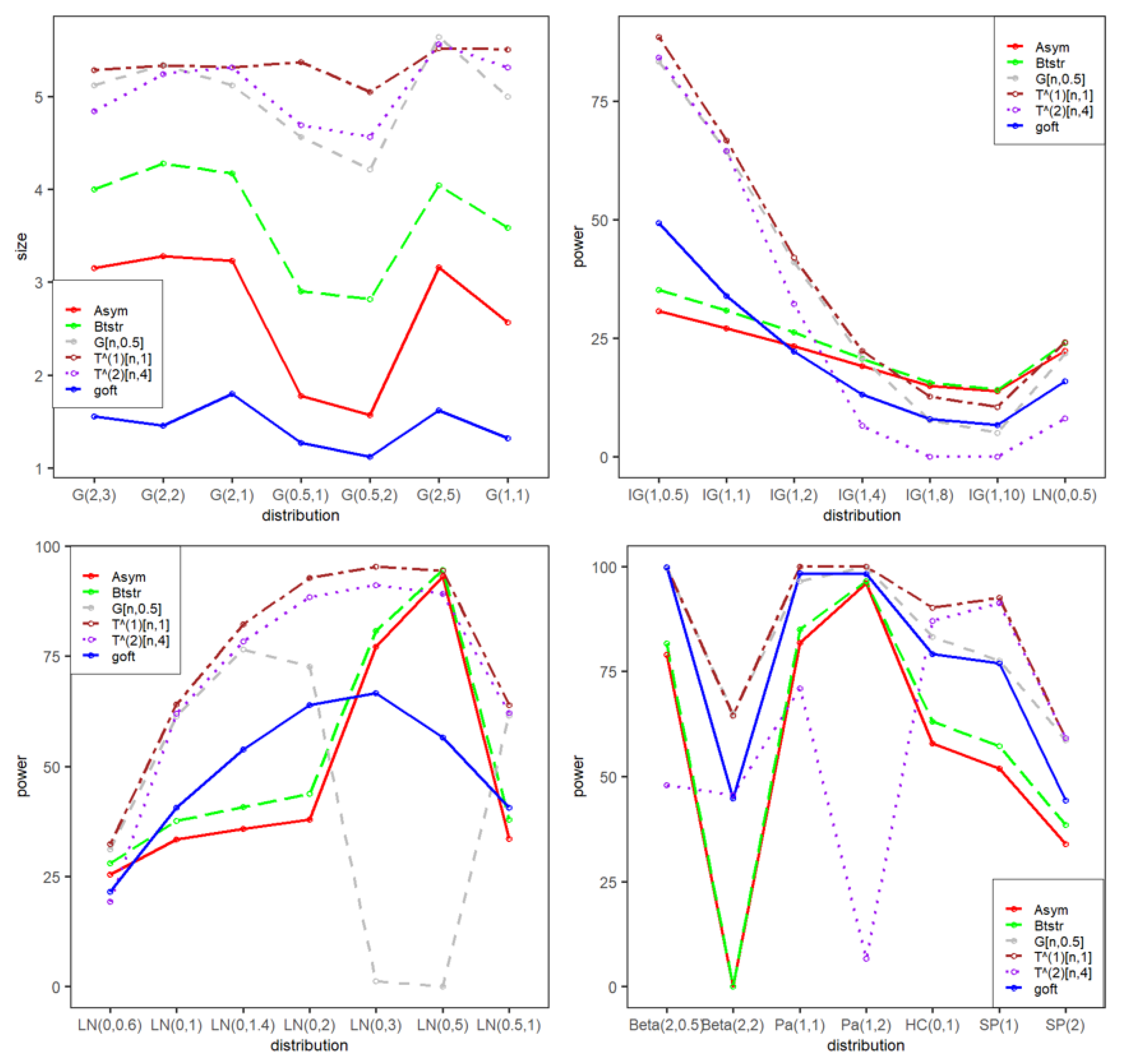
The results are listed in

Table 1. Percentage of 10,000 Monte Carlo samples declared to be significant by various tests for the gamma distribution ($n=50,\alpha =0.05$). MLE $\widehat{\mathbf{\nu }}$ was used.

Alternative	Asym	Btstr	${\mathit{G}}_{\mathit{n},0.5}$	${\mathit{T}}_{\mathit{n},1}^{\left(1\right)}$	${\mathit{T}}_{\mathit{n},4}^{\left(2\right)}$	Goft
$\mathrm{G}\mathrm{a}\mathrm{m}\mathrm{m}\mathrm{a}(2,3)$	3.15	4.00	5.12	5.28	4.84	1.56
$\mathrm{G}\mathrm{a}\mathrm{m}\mathrm{m}\mathrm{a}(2,2)$	3.28	4.28	5.34	5.33	5.24	1.46
$\mathrm{G}\mathrm{a}\mathrm{m}\mathrm{m}\mathrm{a}(2,1)$	3.23	4.17	5.12	5.31	5.31	1.80
$\mathrm{G}\mathrm{a}\mathrm{m}\mathrm{m}\mathrm{a}(0.5,1)$	1.78	2.90	4.56	5.37	4.69	1.27
$\mathrm{G}\mathrm{a}\mathrm{m}\mathrm{m}\mathrm{a}(0.5,2)$	1.57	2.82	4.21	5.05	4.56	1.12
$\mathrm{G}\mathrm{a}\mathrm{m}\mathrm{m}\mathrm{a}(2,5)$	3.16	4.04	5.64	5.52	5.56	1.62
$\mathrm{G}\mathrm{a}\mathrm{m}\mathrm{m}\mathrm{a}(1,1)$	2.57	3.59	5.00	5.50	5.31	1.32
$\mathrm{I}\mathrm{G}(1,0.5)$	30.80	35.29	83.47	88.62	84.22	49.31
$\mathrm{I}\mathrm{G}(1,1)$	27.18	30.89	64.42	66.77	64.51	34.00
$\mathrm{I}\mathrm{G}(1,2)$	23.40	26.31	41.09	42.08	32.27	22.32
$\mathrm{I}\mathrm{G}(1,4)$	19.15	20.69	20.85	22.40	6.68	13.19
$\mathrm{I}\mathrm{G}(1,8)$	15.05	15.73	7.76	12.75	0.04	8.07
$\mathrm{I}\mathrm{G}(1,10)$	13.87	14.21	5.05	10.54	0.01	6.76
$\mathrm{L}\mathrm{N}(0,0.5)$	22.45	24.10	21.82	24.18	8.14	16.03
$\mathrm{L}\mathrm{N}(0,0.6)$	25.48	27.98	31.16	32.31	19.24	21.47
$\mathrm{L}\mathrm{N}(0,1)$	33.39	37.68	61.40	64.00	62.02	40.58
$\mathrm{L}\mathrm{N}(0,1.4)$	35.75	40.74	76.55	82.31	78.36	53.79
$\mathrm{L}\mathrm{N}(0,2)$	37.94	43.83	72.60	92.81	88.46	63.86
$\mathrm{L}\mathrm{N}(0,3)$	77.09	80.80	1.24	95.38	91.10	66.60
$\mathrm{L}\mathrm{N}(0,5)$	93.02	94.62	0.00	94.43	89.16	56.50
$\mathrm{L}\mathrm{N}(0.5,1)$	33.51	37.93	61.50	63.96	62.18	40.60
$\mathrm{B}\mathrm{e}\mathrm{t}\mathrm{a}(2,0.5)$	78.96	81.64	99.63	99.82	48.00	99.72
$\mathrm{B}\mathrm{e}\mathrm{t}\mathrm{a}(2,2)$	0.00	0.01	64.88	64.49	45.64	44.75
$\mathrm{P}\mathrm{a}(1,1)$	81.80	84.91	96.43	99.98	70.99	98.43
$\mathrm{P}\mathrm{a}(1,2)$	95.97	96.44	99.94	99.89	6.60	98.17
$\mathrm{H}\mathrm{C}(0,1)$	57.89	63.01	83.22	90.19	87.04	79.14
$\mathrm{S}\mathrm{P}\left(1\right)$	51.95	57.19	77.58	92.49	91.34	76.93
$\mathrm{S}\mathrm{P}\left(2\right)$	33.99	38.51	58.67	59.07	59.05	44.37

For all alternatives (i.e., except the gamma), the best performing result in each row is given in bold face.

and

Table 2. Percentage of 10,000 Monte Carlo samples declared to be significant by various tests for the gamma distribution ($n=100,\alpha =0.05$). MLE $\widehat{\mathbf{\nu }}$ was used.

Alternative	Asym	Btstr	${\mathit{G}}_{\mathit{n},0.5}$	${\mathit{T}}_{\mathit{n},1}^{\left(1\right)}$	${\mathit{T}}_{\mathit{n},4}^{\left(2\right)}$	Goft
$\mathrm{G}\mathrm{a}\mathrm{m}\mathrm{m}\mathrm{a}(2,3)$	3.54	4.31	5.14	5.03	4.94	2.06
$\mathrm{G}\mathrm{a}\mathrm{m}\mathrm{m}\mathrm{a}(2,2)$	3.73	4.62	4.96	5.11	5.47	2.04
$\mathrm{G}\mathrm{a}\mathrm{m}\mathrm{m}\mathrm{a}(2,1)$	4.17	5.18	5.21	5.16	5.11	2.33
$\mathrm{G}\mathrm{a}\mathrm{m}\mathrm{m}\mathrm{a}(0.5,1)$	2.25	3.69	4.84	5.38	5.24	1.97
$\mathrm{G}\mathrm{a}\mathrm{m}\mathrm{m}\mathrm{a}(0.5,2)$	2.62	4.15	4.52	5.04	4.68	2.07
$\mathrm{G}\mathrm{a}\mathrm{m}\mathrm{m}\mathrm{a}(2,5)$	4.05	4.74	5.53	5.50	5.53	2.31
$\mathrm{G}\mathrm{a}\mathrm{m}\mathrm{m}\mathrm{a}(1,1)$	3.07	4.18	4.78	5.34	5.48	2.01
$\mathrm{I}\mathrm{G}(1,0.5)$	47.21	52.27	99.01	99.67	92.70	84.76
$\mathrm{I}\mathrm{G}(1,1)$	41.67	46.02	92.50	94.77	84.11	67.27
$\mathrm{I}\mathrm{G}(1,2)$	37.00	40.15	71.20	74.37	50.81	47.06
$\mathrm{I}\mathrm{G}(1,4)$	30.66	32.73	41.35	45.33	5.08	29.07
$\mathrm{I}\mathrm{G}(1,8)$	23.39	24.15	17.39	23.86	0.01	16.69
$\mathrm{I}\mathrm{G}(1,10)$	21.10	21.68	12.27	19.75	0.00	13.89
$\mathrm{L}\mathrm{N}(0,0.5)$	35.94	38.17	40.71	45.37	6.72	33.24
$\mathrm{L}\mathrm{N}(0,0.6)$	42.02	44.92	55.53	59.12	27.88	44.23
$\mathrm{L}\mathrm{N}(0,1)$	54.04	57.73	89.24	91.49	77.23	73.54
$\mathrm{L}\mathrm{N}(0,1.4)$	57.54	62.26	97.10	98.49	87.61	86.47
$\mathrm{L}\mathrm{N}(0,2)$	58.01	64.14	77.64	99.77	91.71	93.12
$\mathrm{L}\mathrm{N}(0,3)$	92.18	93.59	0.05	99.97	99.51	95.82
$\mathrm{L}\mathrm{N}(0,5)$	98.36	98.77	0.00	99.96	99.61	93.74
$\mathrm{L}\mathrm{N}(0.5,1)$	54.00	58.51	89.12	91.41	77.58	73.87
$\mathrm{B}\mathrm{e}\mathrm{t}\mathrm{a}(2,0.5)$	99.03	99.25	100.00	100.00	54.70	100.00
$\mathrm{B}\mathrm{e}\mathrm{t}\mathrm{a}(2,2)$	0.63	5.42	92.12	92.43	78.20	90.08
$\mathrm{P}\mathrm{a}(1,1)$	95.05	95.93	94.74	100.00	44.17	100.00
$\mathrm{P}\mathrm{a}(1,2)$	99.91	99.92	100.00	100.00	0.49	100.00
$\mathrm{H}\mathrm{C}(0,1)$	81.95	84.71	88.58	99.31	71.40	98.00
$\mathrm{S}\mathrm{P}\left(1\right)$	75.69	79.69	78.12	99.77	80.91	97.55
$\mathrm{S}\mathrm{P}\left(2\right)$	57.81	62.56	85.02	84.67	72.94	76.30

For all alternatives (i.e., except the gamma), the best performing result in each row is given in bold face.

, where the best performing tests with respect to the power—for each distribution and sample size—are highlighted in bold face for easy reference. Graphical representations of these results are provided in Figure 1 and Figure 2. In these tables and graphs, we use the abbreviations Asym and Btstr for asymptotic and bootstrap, respectively.

According to the results, we conclude the following:

• The empirical size of the test proposed in this paper got closer to the nominal level of 0.05 as the sample size increased.
• The empirical power of the tests increased, as expected, as the sample size increased.
• No test yielded the highest power against all alternatives analyzed, i.e., no test showed uniform superiority over the others, as indeed was expected according to the theoretical results in [31].
• For the $\mathrm{I}\mathrm{G}(1,\lambda )$ model, the larger $\lambda$ was, the better the performance of our gof test was with respect to the other tests considered in the simulation study. However, for the remaining alternative distributions, tests $G_{n,0.5}$ and $T_{n,1}^{\left(1\right)}$ performed better than the proposed test.

4.2. Numerical Examples for the Modified Bessel-Type NEF

In this subsection, we consider some numerical studies in which we applied the gof test to the modified Bessel NEF. These include a simulation study to assess nominal level attainment as well as the analysis of two real data sets. We re-emphasize the point that to the best of our knowledge, it is the first time that a gof test is proposed for such an NEF.

The modified Bessel densities can be either expressed with the modified Bessel function of the second kind of order $1/3$ or with the series expansion given in (2).

Its density series expansion is given by

$$\begin{array}{ccc}\hfill f(x;a,\theta )& =& -exp\left\{\theta x+\frac{2}{a}{\left[-\frac{3}{2}a\theta \right]}^{1/3}\right\}\hfill \\ & & \times \frac{1}{\pi }\sum _{k=0}^{\infty }\frac{{(-1)}^k}{k!}sin\left(\frac{\pi k}{3}\right)3^{\frac{k}{3}}{\left(\frac{2}{a}\right)}^{\frac{2k}{3}}\frac{1}{x^{k/3+1}}\Gamma \left(\frac{k}{3}+1\right),\hfill \\ & & x>0,\theta <0,a>0,\hfill \end{array}$$

where its log-likelihood based on a random sample $(x_1,...,x_n)$ of size n has the form

$$\begin{array}{ccc}\hfill L(a,\theta )& =& \theta \sum _{i=1}^n{x}_i+n\frac{2}{a}{\left[-\frac{3}{2}a\theta \right]}^{1/3}\hfill \\ & & +\sum _{i=1}^{n}log\left\{-\frac{1}{\pi }\sum _{k=0}^{\infty }\frac{{(-1)}^k}{k!}sin\left(\frac{\pi k}{3}\right)3^{\frac{k}{3}}{\left(\frac{2}{a}\right)}^{\frac{2k}{3}}\frac{1}{x_i^{k/3+1}}\Gamma \left(\frac{k}{3}+1\right)\right\}.\hfill \end{array}$$

The maximum likelihood estimators of parameters $\theta$ and a are obtained as the solution of a system of two equations based on the partial derivatives of the log-likelihood function,

$$\frac{\partial L(a,\theta )}{\partial \theta }=0\mathrm{and}\frac{\partial L(a,\theta )}{\partial \theta }=0,$$

where

$$\begin{array}{cc}\hfill \frac{\partial L(a,\theta )}{\partial \theta }=& \sum _{i=1}^n{x}_i-n{\left[-\frac{3}{2}a\theta \right]}^{-\frac{2}{3}},\hfill \\ \hfill \frac{\partial L(a,\theta )}{\partial a}=& -\frac{2n}{a^2}{\left[-\frac{3}{2}a\theta \right]}^{\frac{1}{3}}-\frac{n\theta }{a}{\left[-\frac{3}{2}a\theta \right]}^{-\frac{2}{3}}\hfill \\ \hfill & -\sum _{i=1}^n\frac{{\sum }_{k=0}^{\infty }\frac{{(-1)}^k}{k!}sin\left(\frac{\pi k}{3}\right)3^{\frac{k}{3}}{2}^{\frac{2k}{3}}\frac{2k}{3}{\left(\frac{1}{a}\right)}^{\frac{2k}{3}+1}\frac{1}{x^{k/3+1}}\Gamma \left(\frac{k}{3}+1\right)}{{\sum }_{k=0}^{\infty }\frac{{(-1)}^k}{k!}sin\left(\frac{\pi k}{3}\right)3^{\frac{k}{3}}{\left(\frac{2}{a}\right)}^{\frac{2k}{3}}\frac{1}{x^{k/3+1}}\Gamma \left(\frac{k}{3}+1\right)}.\hfill \end{array}$$

For references on this density, see p. 155 in [32] and [33]. Surprisingly enough, this density has various applications in diffusion and queuing theories (c.f., [34]).

We begin with a small-scale simulation study to assess type 1 error attainment (for nominal level $\alpha =0.05$) under the modified Bessel distribution. We considered six different choices of $\mathrm{B}\mathrm{e}\mathrm{s}\mathrm{s}\mathrm{e}\mathrm{l}(\mu ,\varphi )$, where $\mu$ is the mean and $\varphi$ is the dispersion. In the bootstrap setting, B = 1000 Monte Carlo samples were generated. The results are provided in

Table 3. Percentage of 10,000 Monte Carlo samples declared to be significant by various tests for the modified Bessel distribution $\mathrm{B}\mathrm{e}\mathrm{s}\mathrm{s}\mathrm{e}\mathrm{l}(\mu ,\varphi )$. MLE $\widehat{\mathbf{\nu }}$ was used, and $\alpha =0.05$.

Alternative	Asym		Btstr
	$\mathbf{n}=\mathbf{20}$	$\mathbf{n}=\mathbf{50}$	$\mathbf{n}=\mathbf{20}$	$\mathbf{n}=\mathbf{50}$
$\mathrm{B}\mathrm{e}\mathrm{s}\mathrm{s}\mathrm{e}\mathrm{l}(1,1)$	1.15	2.70	2.10	3.70
$\mathrm{B}\mathrm{e}\mathrm{s}\mathrm{s}\mathrm{e}\mathrm{l}(2,1)$	0.61	1.71	1.10	2.70
$\mathrm{B}\mathrm{e}\mathrm{s}\mathrm{s}\mathrm{e}\mathrm{l}(0.5,1)$	1.63	2.64	2.50	3.20
$\mathrm{B}\mathrm{e}\mathrm{s}\mathrm{s}\mathrm{e}\mathrm{l}(1,2)$	0.35	3.26	0.40	3.70
$\mathrm{B}\mathrm{e}\mathrm{s}\mathrm{s}\mathrm{e}\mathrm{l}(0.5,2)$	0.66	2.09	1.20	3.10
$\mathrm{B}\mathrm{e}\mathrm{s}\mathrm{s}\mathrm{e}\mathrm{l}(1,0.5)$	2.30	3.28	3.60	4.10

. We observed that the nominal level attainment improved as n increased and was better for the bootstrap version than for the asymptotic version. We leave a detailed assessment of the test power to further research and turn instead to real data examples.

The first considered data set represents the marks of slow-pace students in mathematics in the final 2003 examination at IIT Kanpur [35]. The second data set, used by [36], is the vinyl chloride data obtained from clean-up gradient-monitoring wells in mg/L. The data sets, which were recently analyzed by [37], are displayed in

Table 4. IIT Kanpur and vinyl chloride data sets investigated in Section 4.2.

IIT Kanpur Data					Vinyl Chloride Data
29	25	50	15	13	5.1	1.2	1.3	0.6	0.5
27	15	18	7	7	2.4	0.5	1.1	8	0.8
8	19	12	18	5	0.4	0.6	0.9	0.4	2
21	15	86	21	15	0.5	5.3	3.2	2.7	2.9
14	39	15	14	70	2.5	2.3	1	0.2	0.1
44	6	23	58	19	0.1	1.8	0.9	2	4
50	23	11	6	34	6.8	1.2	0.4	0.2
18	28	34	12	37
4	60	20	23	40
65	19	31

. Some basic summary statistics are provided in

Table 5. Summary statistics for IIT Kanpur and vinyl chloride data sets.

	IIT Kanpur Data	Vinyl Chloride Data
Sample size	48	34
Mean	25.90	1.88
Median	19.5	1.15
Standard deviation	18.60	1.95
Inter-quartile range	20	1.98

, indicating considerable skewness to the right.

The p-values for the test statistic in the special case of ${\gamma }_0=2.5$ for these two data sets are given in

Table 6. Results of p-values for the test statistic in the special case of ${\gamma }_0=2.5$ for the two data sets.

	IIT Kanpur Data	Vinyl Chloride Data
Asym	0.767	0.849
Btstr	0.493	0.431

. These p-values indicate that for these data sets, the null hypothesis of the modified Bessel distribution should not be rejected.

5. Conclusions

In this manuscript, we were interested in testing the hypothesis that a given distribution corresponds to a specific ${\mathrm{T}\mathrm{B}\mathrm{E}}_{\gamma }$ model, for fixed $\gamma \in \mathbb{R}∕[0,1)$ and unspecified population parameters. Goodness-of-fit tests are typically based on characterization properties. In our developments, the property $S_r\left(\gamma \right)=0$, as displayed in Propositions 1 and 2, is based on existing relations among the first three cumulants (when using $r=1$) of the null distribution. We demonstrate how $S\left(\gamma \right)\equiv S_1\left(\gamma \right)$ can be estimated and that its squared value produces a statistic that asymptotically approximates 0 under the null hypothesis and whose null distribution is a (scaled) chi-squared distribution with one degree of freedom. The scaling factor depends on distributional moments of the true distribution and needs to be estimated using the data at hand, for instance, with maximum likelihood. While the asymptotic chi-squared property allows the computation of theoretical critical values for the test problem of interest to be performed, we also developed a bootstrap version of the test and demonstrated in our simulation study that this leads to better power and nominal level attainment than those obtained with its theoretical counterpart. Under all of the scenarios, the nominal level attainments and powers increased as the sample size increased.

When the null distribution was gamma, we found that the empirical size of the test proposed in this paper got closer to the nominal level of $0.05$ as the sample size increased, while the empirical power of the test increased, as expected, as the sample size increased. Compared with existing gof tests, it is concluded that for the $IG(1,\lambda )$ alternative, the test proposed in this paper performs better as the value of $\lambda$ gets larger. However, for the remaining alternative distributions considered, the existing tests perform better than the test proposed here. Finally, a detailed simulation study for the special case of modified Bessel and Whittaker distribution, i.e., when ${\gamma }_0=2.5,4$, is a problem to be investigated in further research.

It is entirely not our claim that our proposed gof test performs uniformly better than any other test—an impossible mission that cannot be claimed or accomplished by any other test. Our gof test, however, is applicable to any member of the huge and uncountable class of the ${\mathrm{T}\mathrm{B}\mathrm{E}}_{\gamma }$ models—the vast majority of which have not even been considered in the literature for any statistical modeling. The gamma distribution example considered in this paper is only presented to demonstrate the wide applicability of our proposed gof test.

It is our deep belief that ${\mathrm{T}\mathrm{B}\mathrm{E}}_{\gamma }$ models will be well utilized in the near future for various statistical modeling purposes. Our proposed gof test establishes at least one step in this direction.

References

1. Bar-Lev, S.K.; Kokonendji, C.C. On the mean value parametrization of natural exponential families—A revisited review. Math. Methods Stat. 2017, 26, 159–175. [Google Scholar] [CrossRef]
2. Tweedie, M.C.K. An index which distinguishes between some important exponential families, 579–604. In Statistics: Applications and New Directions, Proceedings of the Indian Statistical Institute Golden Jubilee International Conference; Ghosh, J.K., Roy, J., Eds.; Indian Statistical Institute: Calcutta, India, 1984. [Google Scholar]
3. Bar-Lev, S.K.; Enis, P. Reproducibility and Natural Exponential Families with Power Variance Functions. Ann. Statist. 1986, 4, 1507–1522. [Google Scholar] [CrossRef]
4. Jørgensen, B. Exponential Dispersion Models. J. R. Stat. Society. Ser. B (Methodol.) 1987, 49, 127–162. [Google Scholar] [CrossRef]
5. Bar-Lev, S.K. Independent, Tough Identical Results: The Class of Tweedie on Power Variance Functions and the Class of Bar-Lev and Enis on Reproducible Natural Exponential Families. Int. J. Stat. Probab. 2020, 9, 30–35. [Google Scholar] [CrossRef]
6. Cohen, J.E.; Huillet, T.E. Taylor’s law for some infinitely divisible probability distributions from population models. J. Stat. Phys. 2022, 188, 33. [Google Scholar] [CrossRef]
7. Kokenendji, C.C.; Touré, A.Y.; Abid, R. On general exponential Weight functions and variation phenomenon. Sankhya A 2022, 84, 924–940. [Google Scholar] [CrossRef]
8. Bar-Lev, S.K.; Casalis, M. A classification of reproducible natural exponential families in the broad sense. J. Theor. Probab. 2003, 16, 175–195. [Google Scholar] [CrossRef]
9. Dunn, P.K.; Smyth, G.K. Series evaluation of Tweedie exponential dispersion model densities. Stat. Comput. 2005, 15, 267–280. [Google Scholar] [CrossRef] [Green Version]
10. Bar-Lev, S.K.; Ridder, A. Monte Carlo Methods for Insurance Risk Computation. Int. J. Stat. Probab. 2019, 8, 55–74. [Google Scholar] [CrossRef]
11. Bar-Lev, S.K.; Stramer, O. Characterizations of natural exponential families with power variance functions by zero regression properties. Probab. Theory Relat. Fields 1987, 76, 509–522. [Google Scholar] [CrossRef]
12. Bar-Lev, S.K.; Bshouty, D.; Van der Duyn Schouten, F.A. Zero regression characterizations of natural exponential families generated by Lévy stable laws - a complementary. Math. Methods Stat. 2004, 13, 356–367. [Google Scholar]
13. Bar-Lev, S.K. Discussion on paper by B. Jorgensen, “Exponential dispersion models”. J. Roy. Stat. Soc. Ser. B 1987, 49, 153–154. [Google Scholar]
14. Good, I.J. C164. The cumulants of the lognormal distribution, including some conjectures. J. Stat. Simul. 1983, 17, 321–328. [Google Scholar] [CrossRef]
15. Wilding, G.E.; Mudholkar, G.S. A gamma goodnes-of-fit test based on characteristic independence of the mean and coefficient of variation. J. Stat. Inference 2008, 138, 3813–3821. [Google Scholar] [CrossRef]
16. Linnik, Y.V. Linear forms and statistical criteria. I, II. Ukrain. Mat. Zh. 1953, 5, 207–243, 247–290. English translation in Sel. Transl. Math. Statist. Prob. 1963, 3, 1–90. (In Russian) [Google Scholar]
17. Nikitin, Y.Y. Tests based on characterizations, and their efficiencies: A survey. Acta Comment.Univ. Tartu. Math. 2017, 21, 3–24. [Google Scholar] [CrossRef] [Green Version]
18. Vasicek, O. A test of normality based on sample entropy. J. Roy. Statist. Soc. B 1976, 38, 54–59. [Google Scholar] [CrossRef]
19. Lin, C.T.; Mudholkar, G.S. A simple test for normality against asymmetric alternatives. Biometrika 1980, 67, 455–461. [Google Scholar] [CrossRef]
20. Mudholkar, G.S.; Lin, C.T. On two applications of characterization theorems to goodness-of-fit. Colloq. Math. Soc. Janos Bolyai 1984, 45, 395–414. [Google Scholar]
21. Mudholkar, G.S.; Natarajan, R.; Chaubey, Y.P. A goodness-of-fit test test for the inverse gaussian distribution using its independence characterization. Sankhya B 2001, 63, 362–374. [Google Scholar]
22. Marchetti, C.E.; Mudholkar, G.S. Characterization theorems and goodness-of-fit test. In Goodness-of-Fit Tests and Model Validity, Statistics for Industry and Technology; Huber-Carol, C., Balakrishnan, N., Nikulin, M.S., Mesbah, M., Eds.; Birkhäuser: Boston, MA, USA, 2002. [Google Scholar]
23. Mudholkar, G.S.; Tian, L. An entropy characterization of the inverse Gaussian distribution and related goodness-of-fit test. J. Statist. Plann. Inference 2002, 102, 211–221. [Google Scholar] [CrossRef]
24. Jiménez-Gamero, M.D.; Milošević, B.; Obradović, M. Exponentiality tests based on Basu characterization. Statistics 2020, 54, 714–736. [Google Scholar] [CrossRef]
25. Milošević, B. Asymptotic efficiency of goodness-of-fit tests based on Too-Lin characterization. Commun. Stat.-Simul. Comput. 2020, 49, 2082–2101. [Google Scholar] [CrossRef] [Green Version]
26. Chhikara, R.S.; Folks, J.L. The Inverse Gaussian Distribution: Theory, Methodology, and Applications; Marcel Dekker: New York, NY, USA, 1989. [Google Scholar]
27. Seshadri, V. The Inverse Gaussian Distribution Statistical Theory and Applications; Springer: New York, NY, USA, 1999. [Google Scholar]
28. Betsch, S.; Ebner, B. A new characterization of the Gamma distribution and associated goodness-of-fit tests. Metrics 2019, 82, 779–806. [Google Scholar] [CrossRef] [Green Version]
29. Henze, N.; Meintanis, S.G.; Ebner, B. Goodness-of-Fit Tests for the Gamma Distribution Based on the Empirical Laplace Transform. Commun. Stat. Theoryand Methods 2012, 41, 1543–1556. [Google Scholar] [CrossRef]
30. Villasenor, J.A.; Gonzalez-Estrada, E. A variance ratio test of fit for Gamma distributions. Stat. Probab. Lett. 2015, 96, 281–286. [Google Scholar] [CrossRef]
31. Janssen, A. Global power functions of goodness of fit tests. Ann. Stat. 2000, 28, 239–253. [Google Scholar] [CrossRef]
32. Oberhettinger, F.; Badil, L. Tables of Laplace Transforms; Springer: New York, NY, USA, 1973. [Google Scholar]
33. Zolotarev, V.M. Expressions of the density of a stable distribution with exponent a greater than one by means of a frequency with exponent 1/a. Dokl. Akad. Nauk SSSR 1954, 98, 735–738. [Google Scholar]
34. Feller, W. An Introduction to Probability Theory and Its Applications 2; Wiley: New York, NY, USA, 1966. [Google Scholar]
35. Gupta, R.D.; Kundu, D. A New Class of Weighted Exponential Distributions. Statistics 2009, 43, 621–634. [Google Scholar] [CrossRef]
36. Bhaumik, D.K.; Kapur, K.; Gibbons, R.D. Testing Parameters of a Gamma Distribution for Small Samples. Technometrics 2009, 51, 326–334. [Google Scholar] [CrossRef]
37. Bar-Lev, S.K. Batsidis, Apostolos and Economou, P. Tweedie, Bar-Lev, and Enis class of leptokurtic distributions as a candidate for modeling real data. Commun. Stat. Case Stud. Data Anal. Appl. 2021, 7, 229–248. [Google Scholar] [CrossRef]
38. Korolyuk, V.S.; Borovskikh, Y.V. Theory of U-Statistics; Kluwer: Dordrecht, The Netherlands, 1994. [Google Scholar]
Figure 1. Power curves of the test statistic for 21 alternative distributions, where the null distribution is gamma. The variance M was estimated using the MLE. This figure corresponds to Table 1 in the main text ( n = 50 ; α = 0.05 ).
Mathematics 11 01603 g001
Figure 2. Power curves of the test statistic for 21 alternative distributions, where the null distribution is gamma. The variance M was estimated using the MLE. This figure corresponds to Table 2 in the main text ( n = 100 ; α = 0.05 ).
Mathematics 11 01603 g002