Article

DESnets: A Graphical Representation for Discrete Event Simulation and Cost-Effectiveness Analysis

by
Carmen María Yago
* and
Francisco Javier Díez
Department of Artificial Intelligence, Universidad Nacional de Educación a Distancia (UNED), 28040 Madrid, Spain
*
Author to whom correspondence should be addressed.
Mathematics 2023, 11(7), 1602; https://doi.org/10.3390/math11071602
Submission received: 28 February 2023 / Revised: 22 March 2023 / Accepted: 24 March 2023 / Published: 26 March 2023

Abstract

:
Cost-effectiveness analysis (CEA) is used increasingly in medicine to determine whether the health benefit of an intervention is worth the economic cost. Discrete event simulation (DES) is playing an increasing role in CEA thanks to several advantages, such as the possibility of modeling time and heterogeneous populations. It is usually implemented with general-purpose programming languages or commercial software packages. To our knowledge, no artificial intelligence technique has been applied to DES for CEA. Our objective is to develop a graphical representation, an algorithm, and a software tool that allows non-programmers to easily build models and perform CEA. We present DESnets (discrete event simulation networks) as a new type of probabilistic graphical model inspired by probabilistic influence diagrams, an algorithm for evaluating and an implementation as an OpenMarkov plug-in. DESnets are compared qualitatively and empirically with six alternative tools using as a running example a model about osteoporosis by the British National Institute for Health and Care Excellence (NICE). In our experiments, the implementation of DESnets allowed the building of a typical DES model declaratively. Its evaluation process ranked among the most efficient. DESnets compare favorably with alternative tools in terms of ease of use, expressive power, transparency, and computational efficiency.

1. Introduction

The goal of cost-effectiveness analysis (CEA) is to determine whether the benefit of an intervention is worth its economic cost. In medicine, effectiveness is measured in clinical units, such as life years gained or relapses avoided. Cost–utility analysis is a particular type of economic evaluation in which effectiveness is measured in quality-adjusted life years (QALYs) [1]. Given that it is usually unfeasible to compare several interventions in a randomized controlled trial, due to budgetary and ethical constraints, CEA is almost always based on models; the choice of a modeling framework depends on the nature of the problem [2,3,4,5]. When time must be explicitly represented, state-transition models are still the most common technique [3,6,7]. In general, they assume that time is discrete (i.e., transitions can only occur at the limit of fixed-length intervals) and they assume the Markov hypothesis, which says that the probability of each future state only depends on the present state, not on past states. However, in some cases these assumptions are not a good approximation.
Discrete event simulation (DES) has been applied since the 1950s to numerous fields of which military, logistics, and supply chain management are but a few examples. In the last two decades DES has also become increasingly popular in health economics, as it is more suitable than Markov models when many attributes are necessary to represent the patient’s state [6,8,9,10,11]. Thus, in a heterogeneous population, the evolution of each patient may depend on sex, age, various risk factors, and, sometimes, on the number and type of past events (for example, the accumulation of fractures in osteoporosis). State-transition models are then inappropriate because the number of states grows exponentially with the number of features. The problem is even harder when some attributes are measured in continuous scales, because discretizing a numeric variable into a small number of intervals reduces the precision of the model, which may lead to inaccurate results. In these cases, DES is more appropriate, as it naturally deals with numeric variables, and patient-level simulation can easily reflect each individual’s whole history.
To the best of our knowledge, no artificial intelligence (AI) technique has been used for this purpose, which may be surprising, given that medicine has always been one of the main fields of AI application. The reason may be that CEA must be based on decision theory [12], which requires an explicit representation of probabilities and decision makers’ values, integrated in causal models able to predict and compare the outcomes of different interventions. Neither rule-based expert systems, which were the most successful AI technique in the 1970s and 1980s, nor machine learning, which is the dominant paradigm nowadays, can reason with causality or with probabilities as human experts do. Only one AI approach is able to combine causal knowledge, probabilities, and values: probabilistic graphical models (PGMs) [13,14]. Developed in the 1980s, they encompass other types of models proposed previously in different fields, such as Markov chains [15], genetic networks [16], the naïve Bayes model [17], Markov decision processes (MDPs) [18], partially observable MDPs (POMDPs) [19], Markov random fields (sometimes called Markov networks) [20], and influence diagrams [21]. (These influence diagrams, proposed by Howard and Matheson, are equivalent to decision trees but more compact, and include numerical parameters for probabilities and utilities. They should not be confused with the influence diagrams in the book of Caro et al. [22], which are merely qualitative.) New PGMs proposed in the field of AI are Bayesian networks [23], dynamic Bayesian networks [24], and factored MDPs [25,26].
Our research group has developed CEA algorithms for three types of PGMs: influence diagrams [27], Markov influence diagrams [28], and decision analysis networks [29,30]. In this paper, we introduce DESnets (discrete event simulation networks) as a new type of PGM, designed for DES, especially for health decision analysis when it is not necessary to model interactions between patients or constraints in the access to clinical resources, as is usually assumed in CEA [8,22,31,32]. They differ from standard PGMs in several ways. One difference is that the graph of a DESnet can contain self-loops (links from a node to itself) and directed cycles. The semantics of nodes and links are also new, and the algorithms for evaluating them are completely different. Their main advantage with respect to other modeling frameworks is the possibility of building complex DES models declaratively and performing CEA with a graphical user interface, without requiring programming skills. For this purpose we have implemented DESnets and an algorithm for evaluating them in a plug-in for OpenMarkov [33], an open source tool for PGMs. The rest of the paper is structured as follows: Section 2 introduces the definition of DESnets and the algorithm for CEA. Section 3 compares them with other frameworks for CEA with DES, first qualitatively and then quantitatively by measuring the effectiveness for seven different implementations of one model: DESnet, R, VBA, Arena, Simul8, TreeAge Pro, and DICE. Finally, the discussion in Section 4 summarizes the advantages and disadvantages of DESnets with respect to alternative tools and Section 5 presents the conclusions and some lines for future work.

2. DESnets: Definition and Algorithm for CEA

In this paper, we use as a running example a model about osteoporosis provided by the Decision Support Unit (DSU) of the British National Institute for Health and Care Excellence (NICE). This was published in [8], a document that provides guidance on patient-level modeling approaches, addressing the use of DES frameworks.

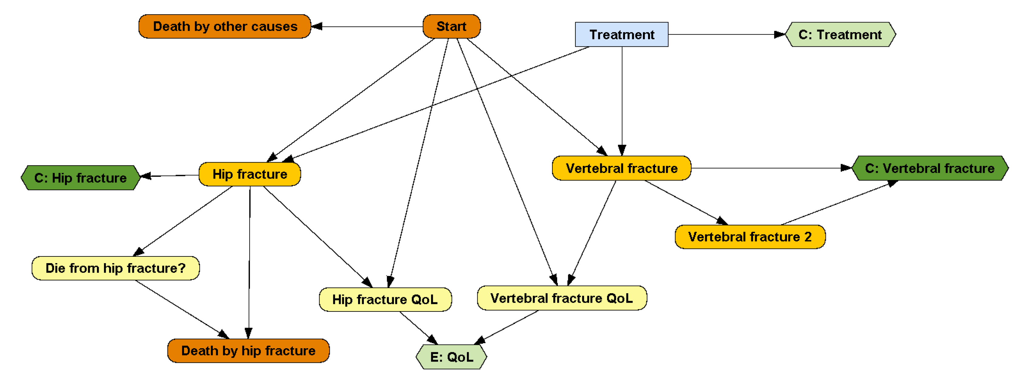
2.1. Representation of DESnets

A DESnet is a probabilistic graphical model (PGM) consisting of a directed graph and several quantitative functions, called potentials. For example, the graph in Figure 1 represents that in the DSU model the patient may suffer from one hip fracture, which may cause death, and up to two vertebral fractures. These fractures result in an immediate cost and a life-long reduction in quality of life. The patient may also die from other causes. There is a treatment, with an annual cost, that may delay the occurrence of hip fracture and the first vertebral fracture.
The following subsections explain in further detail the components of DESnets.

2.1.1. DESnet Nodes

Every node in the graph of a DESnet represents a variable (a property of the system, in this case, the patient), so we will use the terms ‘node’ and ‘variable’ interchangeably. We will denote every variable with a capital letter (X) and its values with lower-case letters (x). A bold upper-case letter  X denotes a set of variables and a bold lower-case letter  x a configuration of them, i.e., the assignment of a value to each variable in  X .
DESnets contain three types of nodes: decisions, probabilistic nodes, and payoffs. A decision node represents a choice made by the decision maker among several options. These nodes are drawn as rectangles and colored in light blue. For example, the node ‘Treatment’ in Figure 1 represents the decision of whether to apply a treatment for osteoporosis or not.
Probabilistic nodes, drawn as rounded rectangles, represent properties and events that are not controlled by the decision maker—at least not directly. Nodes colored in yellow represent chance variables and those in orange represent events. Chance variables represent system properties. For example, ‘Hip fracture QoL’ and ‘Vertebral fracture QoL’ are numeric chance variables representing how the quality of life is affected by the two types of fractures. ‘Die from hip fracture?’ is a Boolean variable that takes the value ‘true’ if, in case of hip fracture, the patient will die. Numeric variables can also be used, for example, to count the number of relapses of a disease or to represent continuous biomarkers.
An event represents something that may occur at a point in time and affects the evolution of the system. A DESnet always has an initial event, called ‘Start’ in Figure 1, and may also have one or several final events, such as ‘Death by hip fracture’ and ‘Death by other causes’. Initial and final events are colored in dark orange. The other events are colored in light orange.
Finally, payoff nodes (in PGMs these nodes are called ‘utility nodes’, but in this paper we call them ‘payoff nodes’ because ‘utility’ might be misunderstood with a particular type of CEA) represent decision maker’s values and are drawn as hexagons. Payoffs can be either one-off costs, such as the upfront expenditure of treating a fracture (nodes ‘C: Hip fracture’ and ‘C: Vertebral fracture’ in our example), or cumulative, such as the the effectiveness (node ‘E: QoL’) or the cost of a chronic treatment (node ‘C: Treatment’). It is possible to distinguish them because a one-off cost is always the consequence of an event. Therefore, payoff nodes having at least one event parent are one-off and the others are cumulative. They are colored dark green and light green, respectively.
Each DESnet has one or several decision criteria and each payoff node corresponds to one of them. In our example, the criterion for the node ‘E: QoL’ is ‘effectiveness’ (in QALYs), while the criterion for the other three payoff nodes is ‘cost’, in monetary units.

2.1.2. DESnet Links

Every links in a DESnet represents causal influence. The type of influence depends on the types of the two nodes it connects. A link E 1 E 2 between two events means that E 1 may cause E 2 . For example, the event ‘Start’ at the beginning of the simulation makes possible the occurrence of ‘Hip fracture’ and ‘Vertebral fracture’.
A link X E , where X is a chance node or a decision and E is an event, means that X affects the probability that E occurs. For example, ‘Treatment = yes’ delays the occurrence of ‘Hip fracture’ and ‘Vertebral fracture’.
A link X Y , where Y is not an event, means that X (which can represent the option chosen for a decision, the occurrence of an event, or the value of a chance variable) affects the value of Y. If X and Y are the same chance node, the link means that the future value of X depends on its previous value.
When an event happens, it affects other parts of the system. In order to determine which variables of the model need to be updated, we will be using the following definition:
Definition 1.
When a directed path from an event node E to another node Y does not contain other event nodes, we say that E is an event-ancestor of Y and Y is an event-descendant of E.
Links are subject to some constraints, explained in Appendix A, to prevent model inconsistencies such as infinite loops in the evaluation.
In the following, we will also use these terms: when the graph has a link X Y , we say that X is a parent of Y and Y is a child of X. The set of parents of a node X is denoted by Pa ( X ) , and  p a ( X ) represents a configuration of them. When there is a directed path from X to Y, we say that X is an ancestor of Y and Y is a descendant of X.

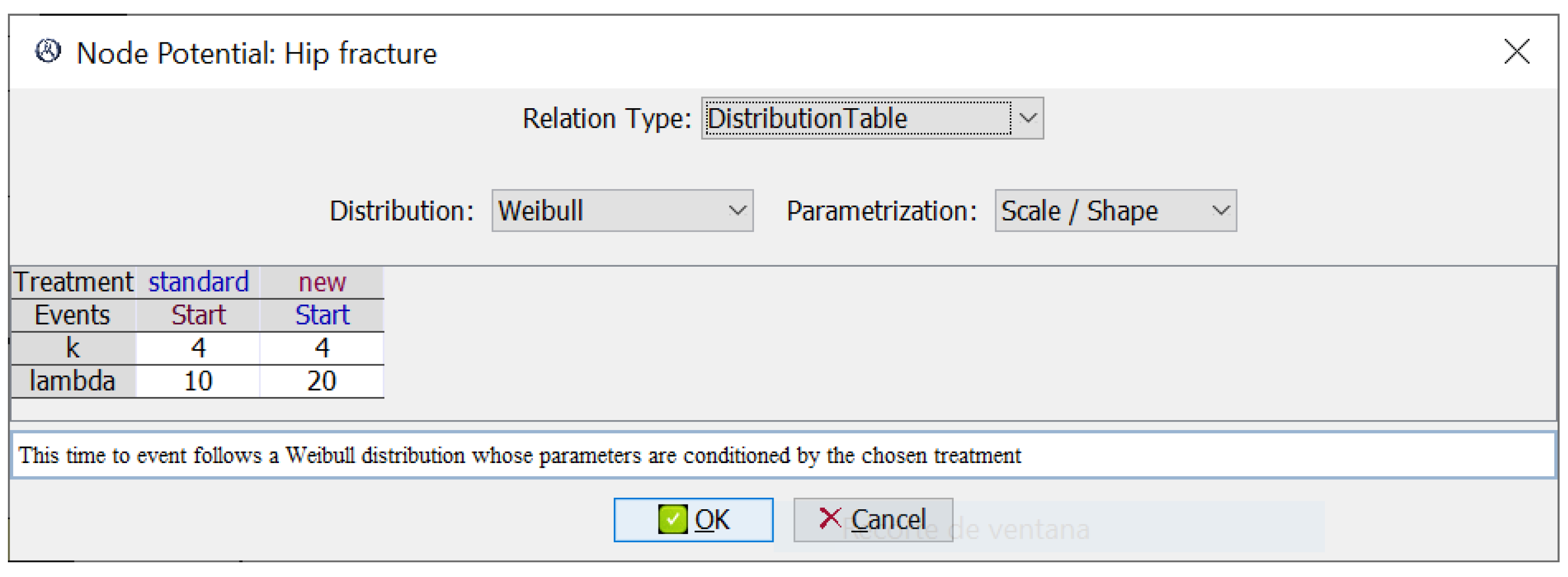
2.1.3. DESnets Potentials

A potential associated with a node is a function that maps each configuration of a set of nodes onto a probability distribution or a real number. The meaning of a potential depends on the type of node to which it is assigned.
Every chance variable X has a potential containing a probabilistic distribution for each configuration of its parents, P ( c | Pa ( C ) ) . For example, P(‘Die From Hip Fracture? = yes’ | ‘Hip fracture’) = 0.05 means that the probability of dying when the event ‘Hip Fracture’ happens is 5%. Some probability functions may be degenerate, i.e., all the values except one have zero probability, which means that the value of C for the configuration Pa ( C ) is determined without uncertainty.
Every payoff node U has a potential that assigns a real number to each configuration of its parents, u ( Pa ( U ) ) . In  the osteoporosis model, the value for the node ‘E: QoL’ is  0.7  times the product of the values of its parents.
Finally, every event E other than ‘Start’ has an associated time-to-event probability density function p E ( t | Pa ( E ) ) , where Pa ( E ) contains at least one event variable  E ; this density represents the probability that E occurs at time t since the occurrence of  E . In our example, the potential in Figure 2 represents the probability of a hip fracture after the event ‘Start’, modeled by two Weibull distributions, one for each treatment.

2.2. Algorithm for Evaluating DESnets

The evaluation of a DESnet consists of computing the value for each decision criterion for a hypothetical set of patients. More specifically, Algorithm 1 is run over K series of N patients; for each patient a simulation is performed for every configuration d of the set of decision nodes D . The core of this algorithm is the iterative generation of the successive events that may occur for each patient, which are put in a queue, called the event calendar, sorted by ascending time of occurrence. In each iteration the first event is taken out and triggered. The simulation begins with the ‘Start’ event and ends when an event (for instance, the patient’s death) ends the simulation, or when the simulation reaches the time horizon.
When an event happens, the variables of the system that depend causally on it are updated using Algorithm 2 and other events may enter the event calendar, in accordance with the time-to-event probabilistic distributions. Payoffs are accrued depending on their type. If an event occurring at time t produces a one-off cost v, the discounted value accrued is
v disc ( v , t , γ ) = 1 ( 1 + γ ) t v ,
where γ is the discount rate. If a cumulative payoff has the value v along the interval ( t 1 , t 2 ) , then the value accrued by the corresponding criterion is
accruedValue U ( v , t 1 , t 2 , γ ) = t 1 t 2 v disc ( v , t , γ ) d t = v 1 ln ( 1 + γ ) 1 ( 1 + γ ) t 1 1 ( 1 + γ ) t 2 ,
If we define
δ = l n ( 1 + γ ) ,
these equations can be rewritten as
v disc ( v , t , γ ) = e δ t v ,
and
accruedValue U ( v , t 1 , t 2 , γ ) = t 1 t 2 v disc ( v , t , γ ) d t = t 1 t 2 v e δ t d t = v e δ t 1 e δ t 2 δ ,
which are sometimes used in the literature.
Algorithm 1: Evaluation of a DESnet for a single patient
Mathematics 11 01602 i001
Algorithm 2: Update event-descendants when an event E happens
Mathematics 11 01602 i002
We can illustrate the execution of Algorithm 1 for the DESnet in Figure 1 with a time horizon of 50 years and an annual discount rate γ = 0.035 . In our model there is only one decision node, ‘Treatment’, with two values: ‘new’ and ‘standard’; in this example, we consider first the configuration d = {new}.
The initialization of the algorithm consists of several steps. First, the value and the accrued value of each of the four payoff nodes is set to 0 (lines 1 and 2). Then, every node that is not a decision and has no event-ancestor is assigned a value (line 3) according to its potential. In this example, ‘C: Treatment’ is set to GBP 500/year, the cost of the new therapy. The variable latestAccrualTime, which indicates when the cumulative payoffs have been accrued, is set to 0 (line 4). The initial event is ‘Start’; after setting its time of occurrence to 0, it is added to the calendar (lines 5 and 6).
When entering the ‘while’ loop, the first event in the calendar, ‘Start’, is extracted and assigned to event. Its occurrence time is 0, which is smaller than the time horizon, so clock is set to 0 (line 9). As clock = latestAccrualTime, the algorithm proceeds to line 13 and updates the event-descendants (see Definition 1) of ‘Start’ in ancestral order, according to Algorithm 2; i.e., ‘Hip fracture QoL’ and ‘Vertebral fracture QoL’ are updated first and then ‘E: QoL’, as follows. The node ‘Hip fracture QoL’ has two parents, which are both events; its potential determines that, when ‘Start’ occurs, this node is assigned the value 1, which means ‘one QALY per year’. For the same reason, the node ‘Vertebral fracture QoL’ is assigned the value 1. The potential for ‘E: QoL’ determines that the value for this node is 0.7 × ‘hip fracture QoL’ בvertebral fracture QoL’; in this case, 0.7 × 1 × 1 = 0.7 (QALYs per year). The next step is to accrue the immediate-payoffs of this event (line 15), which in this case are none.
Then, the events that are children of ‘Start’, namely ‘Hip fracture’ and ‘Vertebral fracture’, are processed (line 19). The potential for ‘Hip fracture’ is a Weibull distribution whose parameters depend on the decision ‘Treatment’, as shown in Figure 2. In the configuration d that we are considering, the value for this decision is the ‘new’ treatment, and the parameters for the Weibull are 4 (shape) and 20 (scale). Let us assume that the result of sampling this distribution is 4.7216 years. This new event, ‘Hip fracture’, is added to the calendar. Similarly, we will assume that when processing the other child event, ‘Vertebral fracture’, the time obtained from its Weibull is 9.1356 years; it is also added to the calendar.
Therefore, in the second iteration of the ‘while’ loop, event will be ‘Hip fracture’ (line 8). Its occurrence time, 4.7216 , is smaller than the time horizon, so clock is set to 4.7216 (line 9). The latest accrual time was still 0, so the cumulative payoffs must be computed for the interval ( 0 , 4.7216 ) —see line 11. There are two cumulative payoffs: ‘E: QoL’ and ‘C: Treatment’. During this interval the effectiveness has been 0.7 QALYs per year, so Equation (5) leads to accruedValue E : QoL ( 0.7 , 0 , 4.7216 , 0.035 ) = 3.0507 QALYs, which is added to the old accrued value, 0. Similarly, for ‘C: Treatment’ we have accruedValue C : Treatment ( 500 , 0 , 4.7216 , 0.035 ) = G B P 2179.04 . After this, latestAccrualTime is set to 4.7216 (line 12), marking the beginning of the next accruing interval.
Now the algorithm updates the event-descendants of ‘Hip fracture’ (line 14), which are two chance nodes (‘Die from hip fracture?’ and ‘Hip fracture QoL’) and two cumulative-payoff nodes (‘E: QoL’ and ‘C: Hip fracture’). ‘Hip fracture QoL’ is updated as in the previous iteration, so that now its value is 0.75 . ‘Die from hip fracture?’ is a Boolean variable having an associated probability distribution, such that the probability of dying (when the parent event occurs) is 5 % . The algorithm takes a random sample, choosing either ‘yes’ with that probability and ‘no’ with 95 % probability. Let us assume that the value obtained is ‘yes’. The new value for ‘E: QoL’ is 0.7 × ‘hip fracture QoL’ × ‘vertebral fracture QoL’ = 0.7 × 0.75 × 1 = 0.5250 QALYs per year. The potential for the immediate-payoff node ‘C: Hip fracture’ determines that the cost of this fracture is GBP 7000; the discounted cost, v disc ( 7000, 4.7216 , 0.035 ) = G B P 5949.63 , given by Equation (1), is added to the accrued value for this node.
Since ‘Hip fracture’ is not final, the algorithm schedules new events (line 19). In this case, the only child event is ‘Death by hip fracture’. According to the potential of this node, when ‘Die from hip fracture?’ = ‘yes’, as we have assumed, the child event occurs immediately after its parent event, which implies that ‘Death by hip fracture’ is added to the calendar with occurrence time set to 4.7216 , which is smaller than the occurrence time of the other scheduled event, ‘Vertebral fracture’.
Therefore, when entering the ‘while’ for the third time, event is ‘Death by hip fracture’. Its occurrence time is smaller than the time horizon, so clock is set to 4.7216 , i.e., its value does not change. This event has no event-descendants (line 14), so it has no immediate-payoff children (line 15). It is a final event, so the calendar is emptied in line 17.
Thus, in the fourth iteration the ‘while’ loop finishes and line 20 computes the value of the two criteria. There is one node for ‘effectiveness’, whose accrued value is 3.0507 QALY. There are three nodes for ‘cost’; the accrued value is GBP 2179.04 for ‘C: Treatment’, GBP 5949.63 for ‘C: Hip fracture’, and GBP 0.00 for ‘C: Vertebral fracture’, so the total cost for this hypothetical patient is GBP 8128.67 .
Then the algorithm should be evaluated for the other configuration of the decisions, d = {standard}.

3. Comparison with Other Frameworks and Software Tools

In this section, we compare DESnets—and their implementation in a plug-in for OpenMarkov—with several alternative frameworks and software tools for CEA with DES:
  • Programming languages (R and VBA);
  • General purpose tools for DES (Arena and Simul8);
  • Software tools specifically designed for this task (TreeAge Pro and DICE).
We first compare them qualitatively, by analyzing their expressive power, easy of use, and transparency, and then quantitatively, by measuring the time required to evaluate the respective versions of the osteoporosis model. The versions for R, VBA, Simul8, TreeAge Pro, and DICE were provided by the DSU, who published the code as Supplementary Material for their technical report [8] and are available at [34]. We implemented the Arena version. Appendix B describes them in detail.

3.1. Qualitative Comparison: Ease of Use, Expressiveness, and Transparency

In CEA, modelers are usually academic researchers, public health agencies, or private companies hired by manufacturers of medical technology—for example, a pharmaceutical laboratory. In the third case, the recipient is a governmental health agency—the paradigm being the above-mentioned NICE—who carefully examines all the information about the new product, including all the clinical evidence and the model used for CEA, and advises the health authorities as to whether the new product should be covered by the public health system. Therefore, when assessing the advantages and disadvantages of a modeling framework, it is necessary to examine both the modeler’s perspective and the recipient’s. For the modeler, the main criteria are the skills and the effort required to build, debug, and maintain a model (maintenance means updating and extending the model when required). For the recipient, the main criterion is transparency, i.e., the possibility of examining whether the hypotheses of the model are sound and whether the implementation is correct.

3.1.1. Programming Languages

DES-based CEA can be implemented in any programming language. R, which was designed for mathematical computations, especially in statistics, is the most widely used for this purpose. Other models have been implemented in Visual Basic for Applications (VBA), Java, or Python (C++ has been used in several CEAs based on Markov models and dynamic transmission models but, to the best of our knowledge, it has never been used for CEA with DES).
When implementing DES in a programming language, the designer has absolute flexibility, which is, in principle, an advantage. The main drawback is that the modeler must implement everything: the simulations (including the generation and management of events), the analyses of the results, such as the accrued payoffs and the incremental cost-effectiveness ratios (ICERs), the sensitivity analyses… Some programming languages have built-in statistical functions and specialized libraries for CEA and/or for DES, which greatly simplify the modeling tasks—for example, R includes several statistical distributions and the package Flexsurv provides some probabilistic functions for parametric survival analysis [35]—but still the implementation of a model for CEA requires strong programming skills and a substantial amount of time to write and debug the code.
The absolute freedom offered by programming languages, which is the main advantage for the modeler, can be a challenge for the recipient who has to examine it and check its validity, because the ability to understand a piece of software code depends, not only on the reader’s skills, but also on the author’s style. Some programmers carefully organize the code with a logical structure, assign meaningful names to variables and functions, and generously annotate the code with useful comments, while others tangle the pieces of code, occasionally choose misleading names for variables and functions, and do not ‘waste’ time on documenting it—we have often experienced it, not only as teachers, but also as researchers when examining open-source programs and CEA models. For example, we can see in Figure A2 and Figure A3 that, although the code for the osteoporosis model in R and in VBA is well structured and carefully commented, understanding it requires some effort and time, even for those with knowledge of these programming languages.
For this reason, the DARTH group [36] is developing a coding framework that offers a template and a set of guidelines aimed at improving the transparency and understandability of decision analysis models in R by standardizing their components, code style, file hierarchy, and naming conventions [37]. All this facilitates significantly the tasks of both modelers and recipients, but still requires significant expertise.
By contrast, DESnets are declarative, i.e., the model only represents real-world variables and relationships among them, thus being separated from the code that implements the evaluation algorithm, which is common to all DESnets. Additionally, the model can be edited with a graphical user interface (GUI). As a consequence, it is possible to build and evaluate complex models without writing a single line of code.
Similarly, the recipient can inspect the model by examining just the graph and the potentials. In particular, every assumption of causal dependence or independence is clearly represented by the presence or the absence of a link, respectively. For the modeler, the main drawback is being limited to the options implemented in the GUI, which may be insufficient in some cases; for example, when some complex correlations present in the data need to be modeled or when the analyst wishes to perform non-standard calculations.

3.1.2. General-Purpose Tools for DES: Arena and Simul8

The two most popular general-purpose tools for DES are Simul8, developed by SIMUL8 Corporation [38], and Arena, by Rockwell Automation [39]. Both have GUIs that allow the building of complex models by combining elementary blocks. They provide many options for generating and managing events, as well as facilities for tracing the evolution of the simulation, which are very useful when debugging the models. Although these features are mainly oriented to simulating production systems, their versatility makes them valuable tools for CEA in health, as they facilitate the modeler’s task and offer the recipient some transparency.
However, being general-purpose entails two main drawbacks for the modeler. First, mastering the use of these tools requires a significant learning effort because, among other reasons, many of the options designed for other applications—such as modeling queues and controlling industrial devices—are rarely used when evaluating health interventions, where usually one patient is evaluated in each simulation. Second, building a model is still a complex task, as shown in Appendix B.4 for Arena and Appendix B.3 for Simul8: the modeler has to lay out an explicit computation plan in the form of a flow diagram (see Figure A4 and Figure A7), then add many formulas and even some code to define each simulation (see Figure A5 for an example in Simul8), and finally write the functions that accrue the payoffs, compute the ICERs, perform the sensitivity analyses, etc. Therefore, even though these tools somehow facilitate the management of events, the programming skills and the time required to build and debug a model is not very different from the case of using a programming language, with the disadvantage of having to adapt the implementation to the ‘philosophy’ of these tools, which may restrict the modeler’s freedom. For the recipient, the flow diagram is a visual aid and the amount of code to be examined is less than in the case of programming languages (because some of the routines for evaluating the model are built into the software tool). However, the effort required to understand the formulas and the code is similar, and additionally requires understanding the intricacies of a commercial product, either Arena or Simul8. In summary, the effort required to perform a CEA using these tools is not smaller than when using a programming language and has the drawbacks of limited flexibility and the need to pay for commercial licenses.
The advantages of DESnets with respect to Arena and Simul8 are the same as those with regard to programming languages: ease for building and evaluating the models and transparency for the recipient. Arena or Simul8 offer more flexibility than DESnets, but only if the modeler implements everything that is not built into them.

3.1.3. TreeAge Pro Healthcare, a Software Tool for CEA with DES

TreeAge Pro Healthcare [40], by TreeAge Pro Software LLC, is a commercial program widely used for decision analysis in medicine. Its basic representation framework are decision trees, which have three main types of nodes: chance, decision, and value. Some years ago, TreeAge added new types of nodes for DES.
The main advantage of this tool is the possibility of building the model with a GUI and then evaluating it automatically: the software runs the simulation, accrues the values, and computes the ICERs, offering several tracing facilities. These advantages are common to DESnets.
The main difference lies in the representation of models. As mentioned above, TreeAge uses an extended version of decision trees, while DESnets are inspired by probabilistic graphical models, so that each node represents a real-world property and links represent causal relations. In contrast, some of the variables and formulas in TreeAge models are introduced just for intermediate calculations. For example, the tree in Figure A9 includes the expression ‘If(N_hip_fract = 0; TimeToHipFracture_Tx; timeHorizon + 1) − (timeCurrent)’, which involves three auxiliary variables—all except timeHorizon—that only make sense during the evaluation of the model. In DESnet, neither are those variables part of the model, nor does the modeler have to write such expressions to execute the simulation, because the model is clearly separated from the code that evaluates it, as mentioned above. Therefore, the effort required and the probability of making mistakes are much lower.
Another advantage from the point of view of representation is that DESnets, owing to their similarity with influence diagrams, are more compact than decision trees: every influence diagram can be expanded into an equivalent decision tree, but the number of branches grows exponentially with the number of variables in the diagram. For instance, our group has built influence diagrams for two medical problems, each having less than 25 variables, whose equivalent decision trees contain tens of thousands of branches [41,42]. TreeAge alleviates this problem by allowing clone nodes, as seen in Figure A9, but in DESnets that workaround is not necessary.
For the recipient, the causal graph of a DESnet clearly shows the relations between the variables and, consequently, the structural hypothesis of the model, while in a decision tree the hypotheses are implicit in the formulas that define the model and, therefore, difficult to observe. Additionally, DESnets require neither auxiliary variables nor expressions for controlling the execution of the simulation, thus making it much easier to assess the correctness of the model.
For the modeler, TreeAge has the same drawback as DESnets with respect to programming languages, i.e., its expressive power is limited to the options implementing in its GUI, as discussed above.

3.1.4. DICE, a Framework with Several Possible Implementations

DICE [43], which stands for ‘Discretely Integrated Condition Event’, is another framework for CEA, especially designed for medicine. It currently supports DES, Markov models, and survival partition models [44]. The first and most widely used implementation is an Excel plug-in with a VBA macro, available for free at [45].
DICE models are clearly structured and the modeler does not need to implement the code for running the simulation and showing the results. However, it still lacks the convenience of a full-fledged GUI, and it is necessary to write a significant number of formulas in the syntax of Excel and DICE, as shown in Figure A12.
This representation is much more complex than when using DESnets. For example, the graph in Figure 1 clearly shows that the probability of ‘Hip fracture’ depends on the treatment, with a time-to-event probability given by the Weibull distributions in Figure 2, and that this event affects the quality of life and the probability of dying. In DICE, this information is encoded in a table (cf. Figure A12) that includes complex formulas for accruing values and doing other computations, as well as some expressions for controlling the simulation flow, which prevents this framework from being purely declarative.
In practice, a drawback of DICE is that the Excel implementation performs noticeably worse than the rest of the tools, as shown below.

3.2. Empirical Comparison

In order to establish the validity of the DESnet formalism, we contrast its implementation in OpenMarkov with the other tools to check that simulation results agree and the evaluation algorithm can be efficiently implemented. We have compared the efficiency of these tools by measuring the time required to evaluate the corresponding version of the osteoporosis model. We used a simulated cohort of 50,000 patients, the same size as in the models provided by the DSU.
Table 1 shows the discounted cost and effectiveness obtained for the two interventions and the running time for each tool, averaged across the 25 series (in this example it does not make sense to compute the ICER because the new treatment dominates the standard one, i.e., it is cheaper and more effective). As expected, all the tools return the same numerical values, within stochastic variations.
Regarding running times, VBA and Arena are the fastest, closely followed by OpenMarkov’s plug-in for DESnets: each of them takes around 1 second for every 50,000-patient simulation. Simul8 needs 3 seconds, i.e., it is around three times slower. TreeAge takes around a half a minute and R almost one minute. The DICE implementation examined was the slowest, as it required almost two and a half hours, probably due to the overhead from using Excel, as confirmed by other studies [46,47,48].

4. Discussion

Several requisites are necessary for a decision analysis tool: ease of use, expressive power, model transparency, and efficiency. First of all, learning to use GUI for DESnets is clearly much easier than learning how to program in a general-purpose language, such as R or VBA, and, in our opinion, easier than using commercial tools for DES, such as Arena or Simul8. Similarly, the effort required to implement a model and conduct a CEA with a GUI for DESnets is much less than when using any of those tools or DICE.
The expressive power of DESnets is more limited than that of programming languages, although it suffices to conduct typical CEAs. However, some complex models, especially those that include non-standard correlations among their parameters, may require a more powerful tool, such as R. Another limitation of DESnets is that the algorithm proposed in this paper can only perform patient-level simulations. When it is necessary to model interactions between patients or constraints in the access to clinical resources, general-purpose simulation tools, such as Arena or Simul8, may be more appropriate.
Model transparency is especially relevant for government agencies that have to assess the validity of CEAs submitted by pharmaceutical laboratories and other manufacturers of health technology. DESnets are more transparent than other tools for two reasons. First, the software for evaluating them is common to all DESnets, and a DESnet consists only of variables that represent real-world concepts and the relationships between them. Both elements are clearly separated. In contrast, a model implemented in a programming language is inseparably embedded in the code that evaluates it and sharing its code does not guarantee transparency [37]. Other tools, such as Arena, Simul8, TreeAge, and DICE also aim at a similar separation of the model from the execution code, but their models include many variables and formulas designed for running the simulations. Second, the causal graph of a DESnet clearly represents the relationships of dependence and independence among the variables, as in standard probabilistic graphical models, such as Bayesian networks, influence diagrams, and factored Markov decisions processes. In contrast, in other tools the assumptions of dependence and independence are implicit in the formulas that relate the variables in the model and are difficult to read out.
Computational efficiency is required to evaluate complex models in a reasonable amount of time. In our empirical comparison, the OpenMarkov plug-in was among the fastest tools, being 3 times faster than Simul8, around 25 faster than TreeAge, 50 times faster than R, and 7600 times faster than DICE, but these results must be taken with a grain of salt, as they depend on the versions evaluated. For example, the R implementation could be improved through the use of vector handling capabilities. In fact, the model by Graves et al. [49]—which is slightly more complex—executes much faster, while Gray et al.’s model for breast cancer [50] and Glover et al.’s model for abdominal aortic aneurysm [51] have similar running time as the DSU implementation of the osteoporosis model despite being much more complex.

5. Conclusions

DESnets are a new visual formalism for performing cost-effectiveness analysis (CEA) with discrete event simulation (DES). The GUI we have developed allows them to be created and evaluated without requiring any programming expertise. We have implemented in this formalism several models published in the literature, including the osteoporosis model used by NICE to illustrate the use of CEA with patient-level simulations.
DESnets compare favorably with alternative frameworks in terms of ease of use, expressive power, transparency, and computational efficiency: the OpenMarkov plug-in was nearly as fast as VBA and Arena, and clearly outperformed Simul8, TreeAge, R, and—especially—the Excel version of DICE. However, a more efficient R version of the osteoporosis model or a different implementation of DICE would have yielded very different results; this is an open issue for future research.
Another line in which we are working is the automatic conversion of DESnets into DICE models. The motivation is that health technology assessment agencies are skeptical about the reliability of new software tools for CEA. Showing that the results of a DESnet agree with those of DICE, which is an increasingly popular tool, already accepted by the British NICE, would help overcome their reluctance.

Supplementary Materials

The following are available at https://bit.ly/3ZIjgVd (accessed on 28 February 2023): the model used as a running example in the OpenMarkov and Arena formats, and the jar file for OpenMarkov with the DESnet plug-in.

Author Contributions

Both authors have contributed to the design of DESnets, and to writing, reviewing, and editing the manuscript. C.M.Y. implemented the OpenMarkov plug-in and ran the experiments. All authors have read and agreed to the published version of the manuscript.

Funding

This work has been supported by grants TIN2016-77206-R and PID2019-110686RB-I00 of the Spanish Government, co-financed by the European Regional Development Fund. C.M.Y. is supported by the UNED and the Spanish Ministry of Science and Innovation through the Technical Support Staff program (‘Personal Técnico de Apoyo’).

Data Availability Statement

The models used in this study are available in the supplementary material and at [34].

Acknowledgments

We thank Glover et al. [51], Graves et al. [49], and Gray et al. [50] for sharing with us their R models, as well as all the authors who have made their software and their models publicly available.

Conflicts of Interest

The authors declare no conflict of interest.

Abbreviations

The following abbreviations are used in this manuscript:
AIArtificial intelligence
CEACost-effectiveness analysis
DESDiscrete event simulation
DESnetDiscrete event simulation network
DSUDecision Support Unit
GUIGraphical user interface
ICERIncremental cost-effectiveness ratio
IDInfluence diagram
MDPMarkov decision process
NICENational Institute for Health and Care Excellence
PGMProbabilistic graphical model
POMDPPartially observable Markov decision process
QALYQuality-adjusted life year

Appendix A. Constraints for DESnets

Every DESnet must fulfill a set of constraints to ensure logical consistency and comply with the evaluation algorithm:
  • There is only one decision because every option (i.e., every state of the decision node) is one of the interventions evaluated in the CEA. This constraint will be relaxed in upcoming versions of the algorithm by taking as the set of interventions the Cartesian product of the states of all the decisions;
  • The initial event is unique and has no parents, because it marks the beginning of the simulation;
  • Any other event has at least one event parent;
  • Final events have no event children because they end the simulation (but they may have chance and payoff nodes as children);
  • Payoff nodes have no children;
  • The domain for time-to-event distributions (density functions) is R + ;
  • Every directed cycle involving more than one node contains at least one event.
The reason for this last constraint is to avoid an infinite evaluation loop. Given that links denote influence, directed cycles, such as the one in Figure A1b, would cause the evaluation of a chance variable to eventually influence itself, thus entering an infinite loop. When an event is present within the cycle (Figure A1b) the problem is avoided, because the influence on an event of a DESnet affects its future time of occurrence, which eliminates the need to compute immediately any further consequences.
Self loops are a special case which does not present the infinite evaluation problem, thanks to their modified semantics, as seen in Section 2.1.2: a link from a chance node C to itself means that the future value of C depends on its previous value, whereas a link from an event E to itself means that E may cause itself to be triggered in the future.
Figure A1. Cycles in a DESnet: (a) is allowed because it contains an event node, whereas (b) is not.
Mathematics 11 01602 g0a1

Appendix B. Implementations of the Osteoporosis Model

We have already described in detail the DESnet version of the osteoporosis model. This appendix describes the other versions and the tools used in the experiments in Section 3.2. The software tools used are:
  • R version 4.1.1, on RStudio 1.4.1717;
  • Microsoft Excel Professional Plus 2016 (for VBA and DICE);
  • Arena version 16.10;
  • TreeAge Pro Healthcare 2022 R1.2.
They were all running on an Intel Core(TM) i7-8565U CPU at 1.80 GHz with 16.0 GB and Windows 10 Home.
Five of the versions of the osteoporosis model used in our experiments were provided by the DSU of the NICE. We introduced some minor modifications to make the results comparable:
  • No time horizon was set, in order to cover the patients’ whole lifespan;
  • Recording of patient-level data was disabled (except for TreeAge, because it was not possible);
  • Batch simulation and simulation timing were enabled.
We have kept those changes to a minimum in all cases, ensuring they do not invalidate the simulation results. Additionally, we built the DESnet and the version in Arena. These are available in the supplementary material.

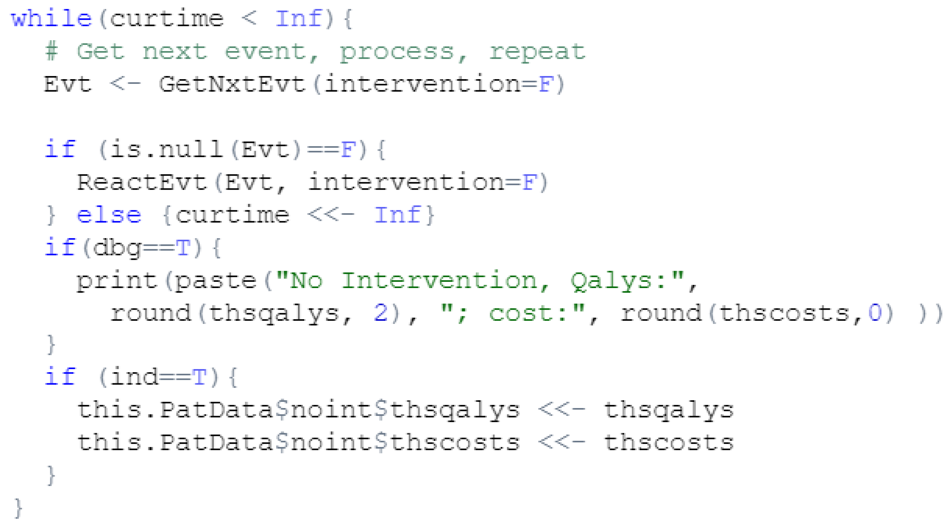
Appendix B.1. R Language

The R version built by the DSU consists of two files. DSU_DesFuntions.R (with 267 lines of code, excluding comments and blank lines) contains the main function, RunSim, and the main event loop (cf. Figure A2), along with seven additional functions. RunSim holds two loops, one for each intervention, which compute the sequence of events and their consequences. The logic of this event processing is generic, since it is agnostic of the specific event triggered at any given time. The file DSU_DES_Script.R (94 lines of code) sets the variables and the simulation parameters, calls the main function, RunSim, and presents the results.
Figure A2. Code for selecting and processing the next event in the R version of the osteoporosis model.
Mathematics 11 01602 g0a2

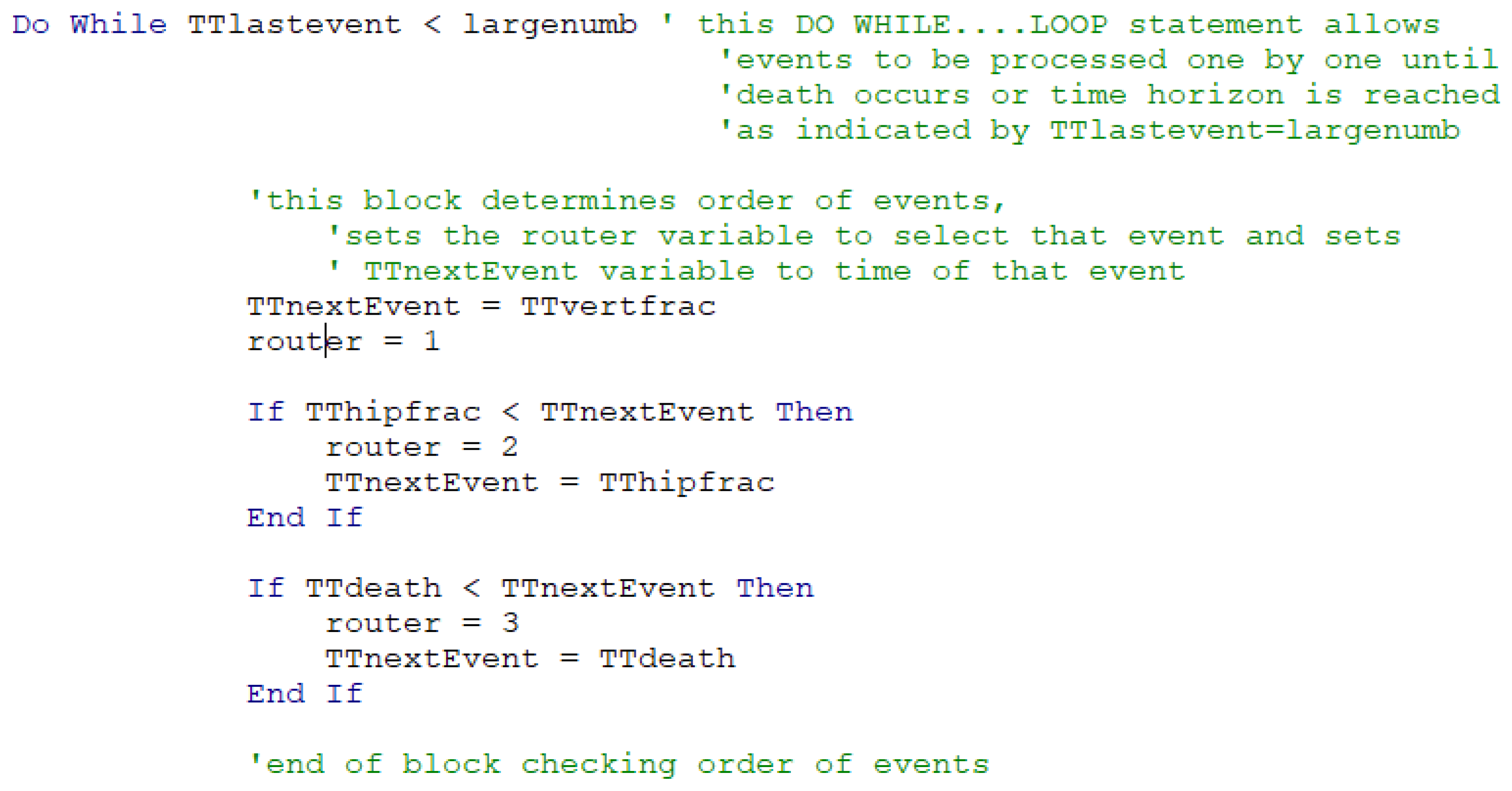
Appendix B.2. VBA Language

This model is embedded in the file Excel_DSU_VBA_DES.xlsx, a macro-enabled workbook that yields its results in Excel sheets. The VBA module, with 233 lines of code, contains a set of declarations and a Sub procedure that carries out the whole simulation. Like in the R model, this code is sufficiently commented.
This procedure generates five sequences of random numbers for N patients; one sequence for each of the four events plus one for the chance of dying from a hip fracture. Then, for each patient and each event the code computes the time to event and enters a loop that, in each iteration, determines which event happens next by comparing their time of occurrence using a series of “If” statements (cf. Figure A3) specific for the events in this model. The consequences of the events are then computed using a “Select Case” statement, which is also tailored to this specific model. This logic differs from that of the R version, which is model-agnostic.
Figure A3. Logic for selecting the next event in the VBA version of the osteoporosis model.
Mathematics 11 01602 g0a3

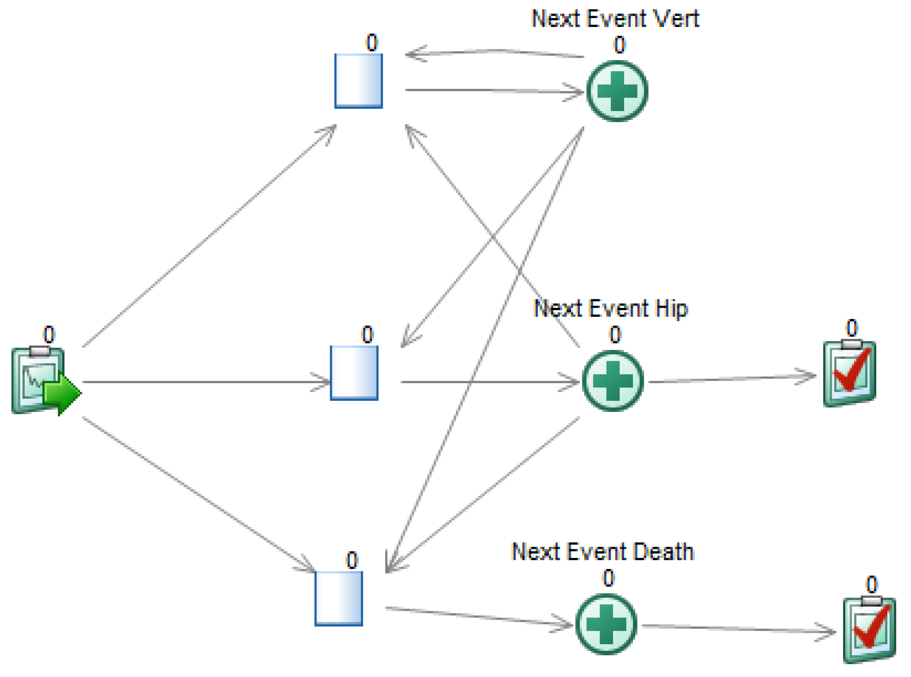
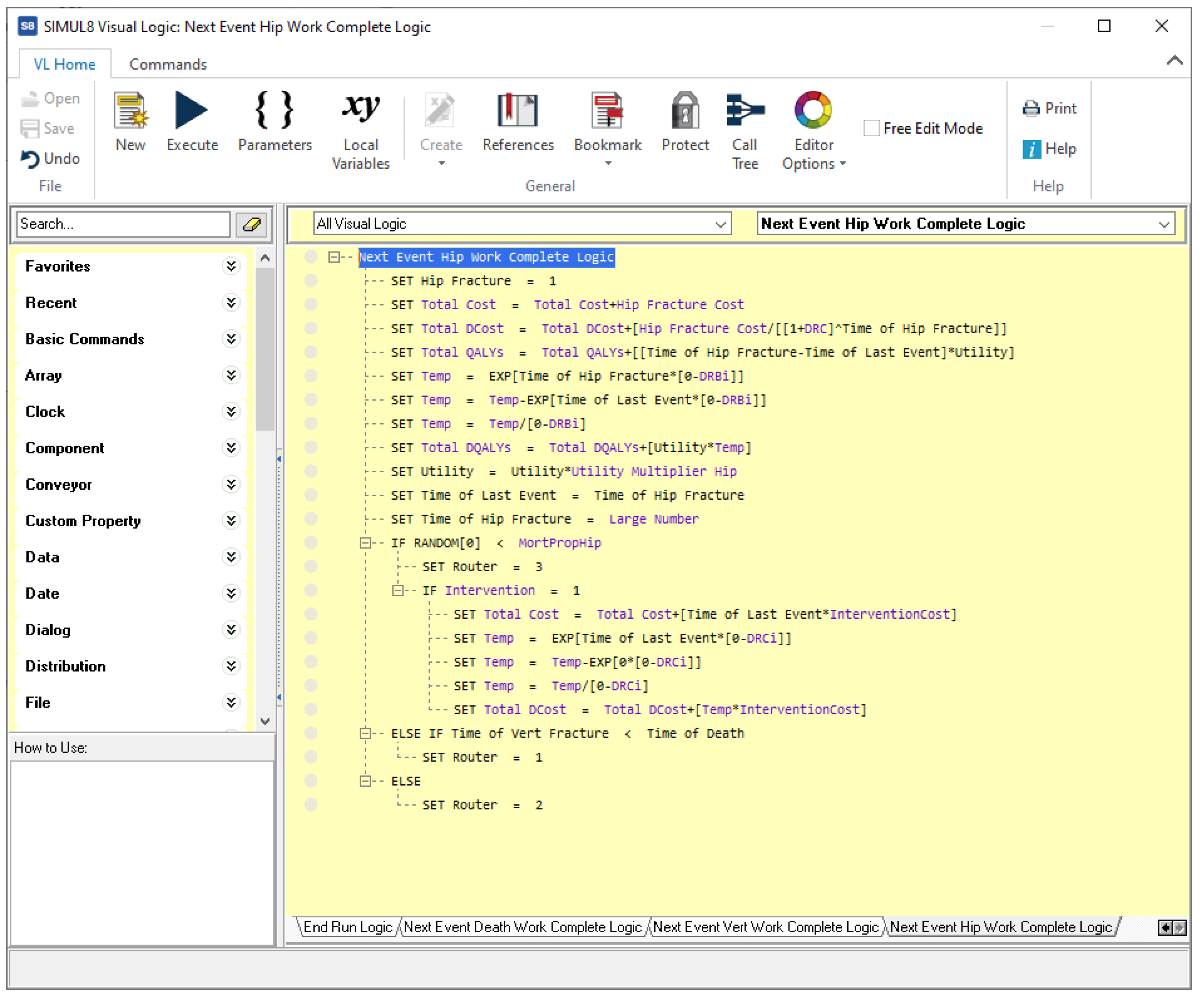
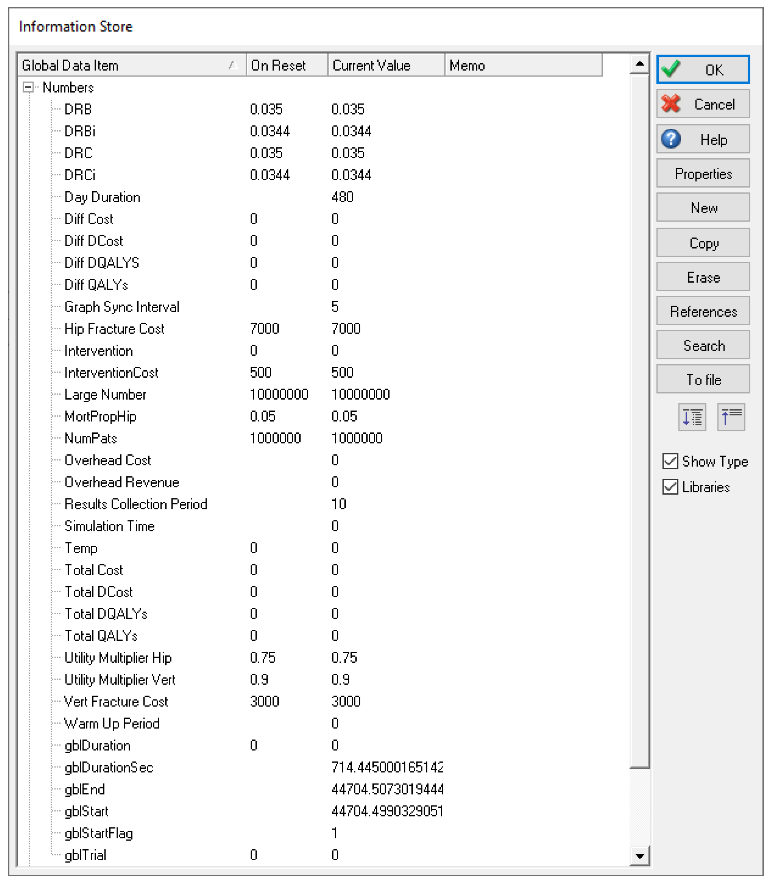
Appendix B.3. Simul8

In Simul8 the model is run twice, one for each intervention. The modeler needs to specify the desired intervention in a variable, prior to simulating. For each intervention, many runs of many patients can be executed in a batch, which is called ‘a trial’.
We can distinguish four main components in the osteoporosis model:
  • A graph, which depicts the simulation flow (cf. Figure A4). There is a start point, where the patients enter the model, three ‘activities’ that represent the main events of the model, and two end points. A queue is necessary to connect each activity with the start point;
  • Visual Logic (VL) code, in several pieces, which specify the behavior of the simulation. For example, Figure A5 shows the code for processing the consequences of the event ‘Hip fracture’. The algorithm implemented in this model is similar to the one in VBA;
  • A set of distributions, selected from Simul8’s catalog;
  • A set of variables, which store model data, auxiliary values, simulation settings, and results; for example, the number of patients to be simulated, the intervention currently examined, the total cost and effectiveness, etc., as shown in Figure A6.
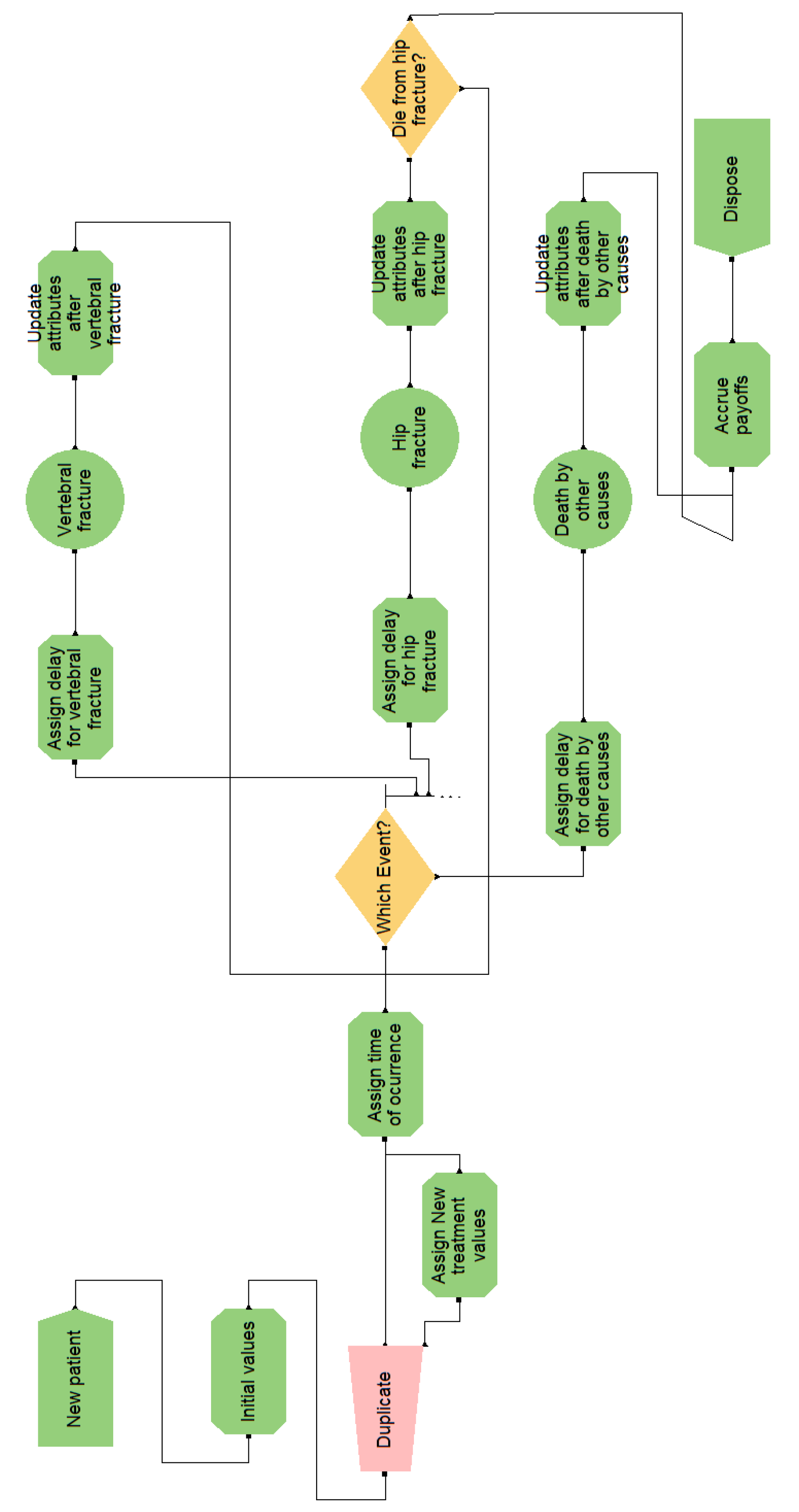
The fact that the simulation settings, including the intervention evaluated, are stored in variables implies that the model must be edited prior to each trial. Additionally, although Simul8 manages the random generators and provides probability distributions, the modeler must ensure that the generators are correctly seeded and set up at the beginning of each trial. This is especially important because each intervention requires a separate trial and trials should be set up consistently across interventions to avoid nuisance variance [22].
The arrows in the Simul8 graph determine the simulation flow; however, being oriented to modeling organizations, it is almost necessary to manually code everything when modeling the course of disease in an individual patient: from computing which event will follow and when, to accruing discounted payoffs. Figure A5 shows a typical example, where, upon an event happening, manual computation must be detailed for accruing costs and effectiveness, keeping track of time, updating the simulation state, and determining the next event.
Figure A4. Graph with the simulation flow for the osteoporosis model in Simul8.
Mathematics 11 01602 g0a4
Figure A5. Code for the ‘Hip fracture’ event in for the osteoporosis model in Simul8.
Mathematics 11 01602 g0a5
Figure A6. Variables for the osteoporosis model in Simul8.
Mathematics 11 01602 g0a6

Appendix B.4. Arena

Given that the book by Caro et al. [22] explains how to perform DES for CEA in Arena, we decided to build a new version of the osteoporosis model to compare it with other tools.
Arena is based on the SIMAN language, which is process-oriented. The main components of this version of the model are:
  • A graph, which constitutes the flow diagram, built with SIMAN blocks. Entities—patients, in our case—flow through the diagram, triggering actions (such as computing values, assigning variables, and accruing payoffs) in the blocks they traverse. For example, the ‘Which Event?’ block, shown in Figure A7, has some embedded logic (cf. Figure A8) for selecting the next event when a patient arrives. The probability distributions are sampled at the ‘Initial values’ block, placed before ‘Duplicate’, in order to reduce nuisance variance. This allows both interventions to be simulated while ensuring that values change only when needed;
  • Variables, which hold the values global to the whole simulation, such as the accrued payoffs;
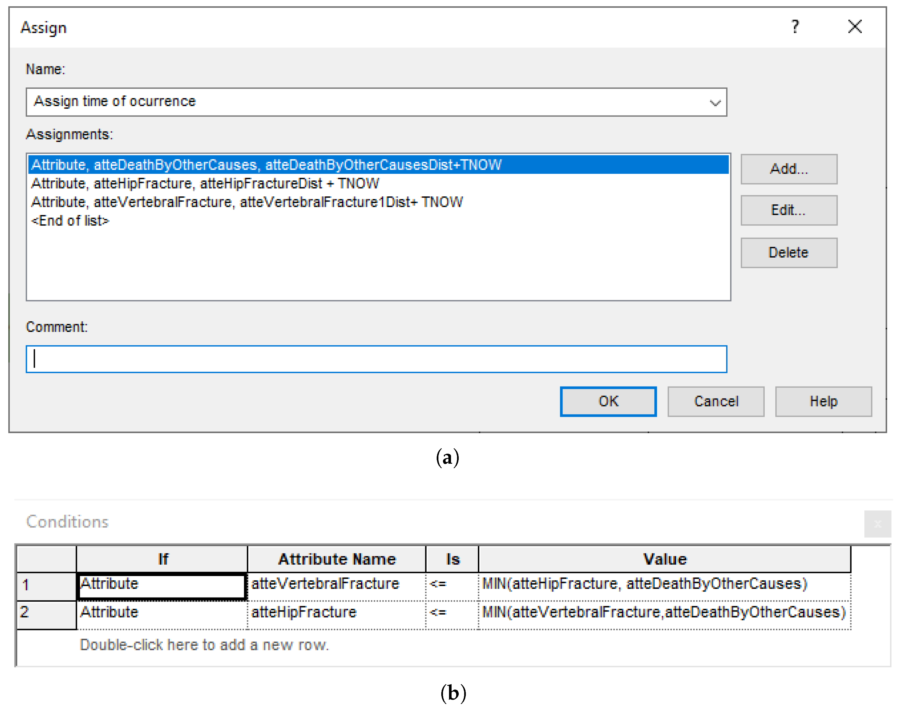
  • Attributes, which hold values for the current patient, including the times of occurrence of the events.
Arena allows the running of multiple simulations in a batch and collecting overall statistics.
Figure A7. Flow diagram for the osteoporosis model in Arena.
Mathematics 11 01602 g0a7
Figure A8. Explicit computations in Arena blocks. (a) Block of type ‘Assign’ for setting the occurrence time of the next events. (b) Block of type ‘Decide’ for selecting the next event.
Mathematics 11 01602 g0a8

Appendix B.5. TreeAge

We can distinguish two main parts in the osteoporosis model:
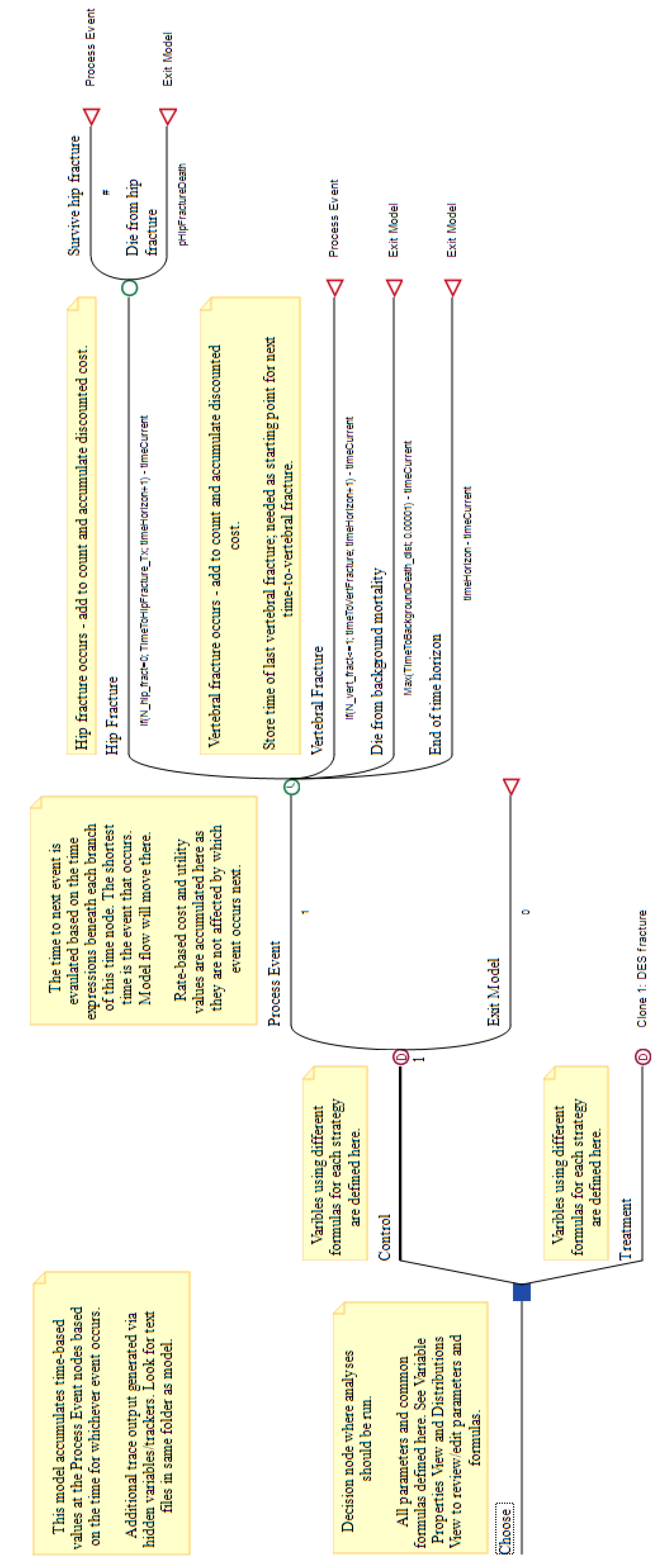
  • A tree, shown in Figure A9. Its root is a decision node for the two interventions, ‘Control’ and ‘Treatment’. The second branch is a clone, with redefined variables;
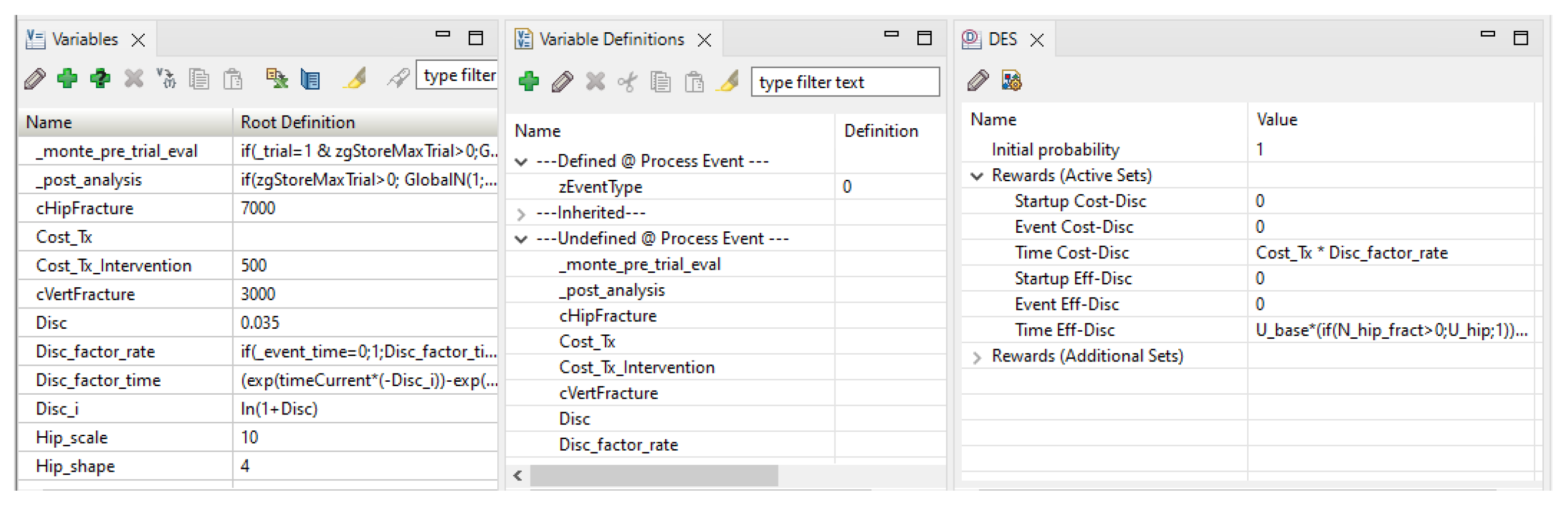
  • The bottom pane, shown in Figure A10, with tabs for different element types: variables, variable definitions, distributions, DES payoffs, etc.
When an event occurs, either the simulation ends or it resumes at the ‘Process Event’ node. The ‘Time’ node, drawn with a clock icon, has one outgoing branch for each event. During the evaluation, the algorithm obtains a time of occurrence for each event and the flow continues on the branch for the event occurring first. This requires controlling manually the events that may occur at most once and those that must be preceded by others; additionally, when an event occurs, the time elapsed must be subtracted from the time to event sampled for each of the other events.
Figure A9. Decision tree for the osteoporosis model in TreeAge. The decision has one subtree for each intervention (here, ‘Control’ and ‘Treatment’). The subtrees perform the DES simulation, as noted by their root being a DES node (circled ‘D’). The top DES node is labelled with ‘1’ because it was the source for cloning the bottom one. Branches in a DES subtree may have a time to event or a probability value; in this case, a ‘#’ symbol represents the complement probability.
Mathematics 11 01602 g0a9
Figure A10. TreeAge’s bottom pane, showing the variables and the DES properties for the ‘Time’ node.
Mathematics 11 01602 g0a10
In our experiment, we detected an issue in the DSU version in TreeAge, which caused a division by zero error when computing ‘Payoff 6’. After a consultation with the DSU, we fixed it. With respect to the execution time shown in Table 1, we should mention that TreeAge generates a large amount of patient-level data to be shown after finishing; this process takes nearly half of the running time for the osteoporosis model, but it cannot be disabled.

Appendix B.6. DICE

The DICE version of the osteoporosis model is implemented in an Excel workbook including the VBA macro that executes the simulation. Some Excel sheets specify the model and others collect the results. The main components of the model are:
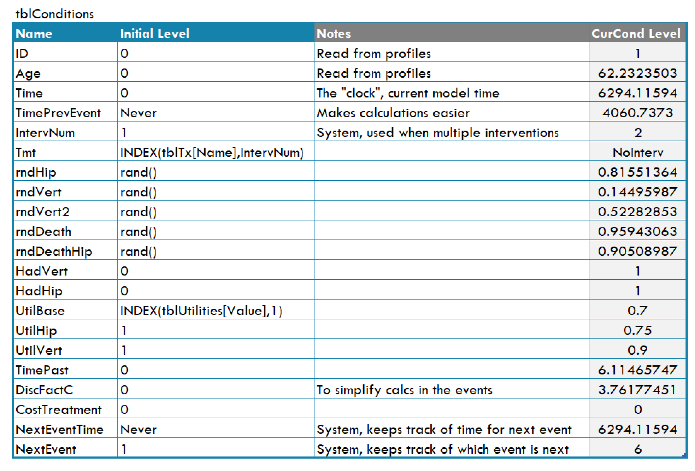
  • Conditions, which are variables used to represent real world magnitudes (for instance, ‘Age’) or to implement the flow control (for example, ‘TimePrevEvent’). Each condition has a name and a value (called ‘level’) and appears as a row in the ‘conditions table’, shown in Figure A11;
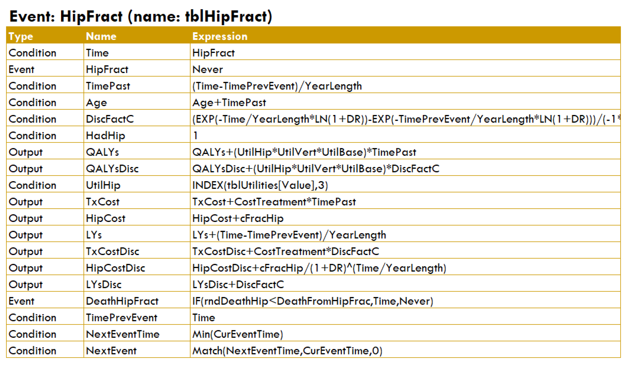
  • Events, each having an associated table (see Figure A12) that indicates how to update the simulation when the event occurs; for example, changing the ‘level’ of some conditions, queuing new events, or calculating some outputs;
  • Outputs. In DICE each output defines a property for which the evaluation will return a value. In this model, the outputs are not only cost and effectiveness but also some other properties, such as the age of death;
  • Results. These are the values (usually numerical) obtained for the different outputs, both patient-level data and accrued values.
Figure A11. Table of conditions for the osteoporosis model in DICE.
Mathematics 11 01602 g0a11
Figure A12. Table for the ‘hip fracture’ event in DICE.
Mathematics 11 01602 g0a12

References

  1. Drummond, M.F.; Sculpher, M.J.; Claxton, K.; Stoddart, G.L.; Torrance, G.W. Methods for the Economic Evaluation of Health Care Programmes, 4th ed.; Oxford University Press: Oxford, UK, 2015. [Google Scholar]
  2. Brennan, A.; Chick, S.E.; Davies, R. A taxonomy of model structures for economic evaluation of health technologies. Health Econ. 2006, 15, 1295–1310. [Google Scholar] [CrossRef] [PubMed]
  3. Caro, J.J.; Briggs, A.H.; Siebert, U.; Kuntz, K.M. Modeling good research practices—Overview: A report of the ISPOR-SMDM Modeling Good Research Practices Task Force-1. Value Health 2012, 15, 796–803. [Google Scholar] [CrossRef] [PubMed] [Green Version]
  4. Degeling, K.; Franken, M.D.; May, A.M.; van Oijen, M.G.; Koopman, M.; Punt, C.J.; IJzerman, M.J.; Koffijberg, H. Matching the model with the evidence: Comparing discrete event simulation and state-transition modeling for time-to-event predictions in a cost-effectiveness analysis of treatment in metastatic colorectal cancer patients. Cancer Epidemiol. 2018, 57, 60–67. [Google Scholar] [CrossRef] [PubMed]
  5. Gibson, E.J.; Begum, N.; Koblbauer, I.; Dranitsaris, G.; Liew, D.; McEwan, P.; Yuan, Y.; Juarez-Garcia, A.; Tyas, D.; Pritchard, C. Cohort versus patient level simulation for the economic evaluation of single versus combination immuno-oncology therapies in metastatic melanoma. J. Med. Econ. 2019, 22, 531–544. [Google Scholar] [CrossRef] [PubMed] [Green Version]
  6. Karnon, J.; Afzali, H. When to use discrete event simulation (DES) for the economic evaluation of health technologies? A review and critique of the costs and benefits of DES. PharmacoEconomics 2014, 32, 547–558. [Google Scholar] [CrossRef] [PubMed]
  7. Zheng, Y.; Pan, F.; Sorensen, S. Modeling treatment sequences in pharmacoeconomic models. PharmacoEconomics 2016, 35, 15–24. [Google Scholar] [CrossRef]
  8. Davis, S.; Stevenson, M.; Tappenden, P.; Wailoo, A. Technical Support Document 15: Cost-Effectiveness Modelling Using Patient-Level Simulation; Technical Report; Decision Support Unit, National Institute for Health and Care Excellence (NICE): London, UK, 2014; Available online: https://www.sheffield.ac.uk/nice-dsu/tsds/patient-level-simulation (accessed on 20 February 2023).
  9. Salleh, S.; Thokala, P.; Brennan, A.; Hughes, R.; Dixon, S. Discrete event simulation-based resource modelling in health technology assessment. PharmacoEconomics 2017, 35, 989–1006. [Google Scholar] [CrossRef]
  10. Sharp, L.; Tilson, L.; Whyte, S.; Ceilleachair, A.O.; Walsh, C.; Usher, C.; Tappenden, P.; Chilcott, J.; Staines, A.; Barry, M.; et al. Using resource modelling to inform decision making and service planning: The case of colorectal cancer screening in Ireland. BMC Health Serv. Res. 2013, 13, 105. [Google Scholar] [CrossRef] [Green Version]
  11. Standfield, L.; Comans, T.; Scuffham, P. Markov modeling and discrete event simulation in health care: A sytematic comparison. Int. J. Technol. Assess. Health Care 2014, 30, 165–172. [Google Scholar] [CrossRef] [Green Version]
  12. von Neumann, J.; Morgenstern, O. Theory of Games and Economic Behavior; Princeton University Press: Princeton, NJ, USA, 1944. [Google Scholar]
  13. Koller, D.; Friedman, N. Probabilistic Graphical Models: Principles and Techniques; The MIT Press: Cambridge, MA, USA, 2009. [Google Scholar]
  14. Pearl, J. Probabilistic Reasoning in Intelligent Systems: Networks of Plausible Inference; Morgan Kaufmann: San Mateo, CA, USA, 1988. [Google Scholar]
  15. Markov, A.A. Rasprostranenie zakona bol’shih chisel na velichiny, zavisyaschie drug ot druga. Izv.-Fiz.-Mat. Obs. Pri Kazan. Univ. 1906, 15, 135–156. [Google Scholar]
  16. Wright, S. Correlation and causation. J. Agric. Res. 1921, 20, 557–585. [Google Scholar]
  17. Warner, H.R.; Toronto, A.F.; Veasy, L.G.; Stephenson, R. A mathematical approach to medical diagnosis: Application to congenital heart disease. JAMA 1961, 177, 177–183. [Google Scholar] [CrossRef] [PubMed]
  18. Bellman, R.E. Dynamic Programming; Princeton University Press: Princeton, NJ, USA, 1957. [Google Scholar]
  19. Åström, K.J. Optimal control of Markov processes with incomplete state estimation. J. Math. Anal. Appl. 1965, 10, 174–205. [Google Scholar] [CrossRef] [Green Version]
  20. Kindermann, R.; Snell, J.L. Markov Random Fields and Their Applications; American Mathematical Society: Providence, RI, USA, 1980. [Google Scholar]
  21. Howard, R.A.; Matheson, J.E. Influence diagrams. In Readings on the Principles and Applications of Decision Analysis; Howard, R.A., Matheson, J.E., Eds.; Strategic Decisions Group: Menlo Park, CA, USA, 1984; pp. 719–762. [Google Scholar]
  22. Caro, J.J.; Möller, J.; Karnon, J.; Stahl, J.; Ishak, J. Discrete Event Simulation for Health Technology Assessment; Chapman and Hall/CRC: Boca Raton, FL, USA, 2015. [Google Scholar] [CrossRef]
  23. Pearl, J. Fusion, propagation and structuring in belief networks. Artif. Intell. 1986, 29, 241–288. [Google Scholar] [CrossRef] [Green Version]
  24. Dean, T.; Kanazawa, K. A model for reasoning about persistence and causation. Comput. Intell. 1989, 5, 142–150. [Google Scholar] [CrossRef]
  25. Boutilier, C.; Dearden, R.; Goldszmidt, M. Stochastic dynamic programming with factored representations. Artif. Intell. 2000, 121, 49–107. [Google Scholar] [CrossRef] [Green Version]
  26. Boutilier, C.; Poole, D. Computing optimal policies for partially observable decision processes using compact representations. In Proceedings of the Thirteenth National Conference on Artificial Intelligence (AAAI’96), Portland, OR, USA, 4–8 August 1996; Clancey, W.J., Weld, D.S., Eds.; AAAI Press/MIT Press: Portland, OR, USA, 1996; pp. 1168–1175. [Google Scholar]
  27. Arias, M.; Díez, F.J. Cost-effectiveness analysis with influence diagrams. Methods Inf. Med. 2015, 54, 353–358. [Google Scholar] [CrossRef] [PubMed] [Green Version]
  28. Díez, F.J.; Yebra, M.; Bermejo, I.; Palacios-Alonso, M.A.; Arias, M.; Luque, M.; Pérez-Martín, J. Markov influence diagrams: A graphical tool for cost-effectiveness analysis. Med. Decis. Mak. 2017, 37, 183–195. [Google Scholar] [CrossRef] [PubMed] [Green Version]
  29. Díez, F.J.; Luque, M.; Bermejo, I. Decision analysis networks. Int. J. Approx. Reason. 2018, 96, 1–17. [Google Scholar] [CrossRef] [Green Version]
  30. Díez, F.J.; Luque, M.; Arias, M.; Pérez-Martín, J. Cost-effectiveness analysis with unordered decisions. Artif. Intell. Med. 2021, 117, 102064. [Google Scholar] [CrossRef]
  31. Caro, J.J.; Möller, J. Advantages and disadvantages of discrete-event simulation for health economic analyses. Expert Rev. Pharmacoecon. Outcomes Res. 2016, 16, 327–329. [Google Scholar] [CrossRef] [PubMed] [Green Version]
  32. Karnon, J.; Stahl, J.E.; Brennan, A.; Caro, J.J.; Mar, J.; Möller, J. Modeling using discrete event simulation: A report of the ISPOR-SMDM Modeling Good Research Practices Task Force-4. Value Health 2012, 15, 821–827. [Google Scholar] [CrossRef] [PubMed] [Green Version]
  33. OpenMarkov. Available online: http://www.openmarkov.org (accessed on 28 February 2023).
  34. Patient-Level Simulation TSD | NICE Decision Support Unit | The University of Sheffield. Available online: https://www.sheffield.ac.uk/nice-dsu/tsds/patient-level-simulation (accessed on 19 February 2023).
  35. Jackson, C. flexsurv: A platform for parametric survival modeling. J. Stat. Softw. 2016, 70. [Google Scholar] [CrossRef] [PubMed] [Green Version]
  36. DARTH—Decision Analysis in R for Technologies in Health. Available online: https://darthworkgroup.com (accessed on 28 February 2023).
  37. Alarid-Escudero, F.; Krijkamp, E.M.; Pechlivanoglou, P.; Jalal, H.; Kao, S.Y.Z.; Yang, A.; Enns, E.A. A need for change! A coding framework for improving transparency in decision modeling. PharmacoEconomics 2019, 37, 1329–1339. [Google Scholar] [CrossRef]
  38. Simul8|Fast, Intuitive Simulation Software for Desktop and Web. Available online: https://www.simul8.com (accessed on 28 February 2023).
  39. Arena Simulation Software. Available online: https://www.rockwellautomation.com/es-es/products/software/arena-simulation.html (accessed on 28 February 2023).
  40. TreeAge Software. Available online: https://www.TreeAge.com (accessed on 28 February 2023).
  41. León, D. A Probabilistic Graphical Model for Total Knee Arthroplasty. Master’s Thesis, Department of Artificial Intelligence, UNED, Madrid, Spain, 2011. [Google Scholar]
  42. Luque, M.; Díez, F.J.; Disdier, C. Optimal sequence of tests for the mediastinal staging of non-small cell lung cancer. BMC Med. Inform. Decis. Mak. 2016, 16, 9. [Google Scholar] [CrossRef] [Green Version]
  43. Caro, J.J. Discretely Integrated Condition Event (DICE) simulation for pharmacoeconomics. PharmacoEconomics 2016, 34, 665–672. [Google Scholar] [CrossRef] [PubMed]
  44. Caro, J.J.; Maconachie, R.; Woods, M.; Naidoo, B.; McGuire, A. Leveraging DICE (Discretely-Integrated Condition Event) simulation to simplify the design and implementation of hybrid models. Value Health 2020, 23, 1049–1055. [Google Scholar] [CrossRef]
  45. Discretely Integrated Condition Event (DICE) Simulation. Available online: https://www.evidera.com/dice (accessed on 19 February 2023).
  46. Arlegui, H.; Nachbaur, G.; Praet, N.; Bégaud, B.; Caro, J.J. Using discretely integrated condition event simulation to construct quantitative benefit-risk models: The example of rotavirus vaccination in France. Clin. Ther. 2020, 42, 1983–1991. [Google Scholar] [CrossRef]
  47. Möller, J.; Davis, S.; Stevenson, M.; Caro, J.J. Validation of a DICE simulation against a discrete event simulation implemented entirely in code. PharmacoEconomics 2017, 35, 1103–1109. [Google Scholar] [CrossRef]
  48. Pennington, B.; Filby, A.; Owen, L.; Taylor, M. Smoking cessation: A comparison of two model structures. PharmacoEconomics 2018, 36, 1101–1112. [Google Scholar] [CrossRef]
  49. Graves, J.; Garbett, S.; Zhou, Z.; Schildcrout, J.S.; Peterson, J. Comparison of decision modeling approaches for health technology and policy evaluation. Med. Decis. Mak. 2021, 41, 453–464. [Google Scholar] [CrossRef] [PubMed]
  50. Gray, E.; Donten, A.; Karssemeijer, N.; Van Gils, C.; Evans, D.G.; Astley, S.; Payne, K. Evaluation of a stratified national breast screening program in the United Kingdom: An early model-based cost-effectiveness analysis. Value Health 2017, 20, 1100–1109. [Google Scholar] [CrossRef] [PubMed] [Green Version]
  51. Glover, M.J.; Jones, E.; Masconi, K.L.; Sweeting, M.J.; Thompson, S.G.; SWAN Collaborators. Discrete event simulation for decision modeling in health care: Lessons from abdominal aortic aneurysm screening. Med. Decis. Mak. 2018, 38, 439–451. [Google Scholar] [CrossRef] [PubMed]
Figure 1. A DESnet for the osteoporosis model. Rectangles (in blue) represent decisions. Rounded rectangles represent probabilistic nodes, either chance variables (in yellow) or events (in orange; initial and final events are colored in dark orange). Hexagons represent payoff nodes, either one-off costs due to events (in dark green) or values that accumulate over time (in light green).
Mathematics 11 01602 g001
Figure 2. Potential for the event ‘Hip fracture’. It has one time-to-event Weibull distribution for each treatment. The scale parameter, λ , is higher for the new treatment because it tends to delay the occurrence of fractures.
Mathematics 11 01602 g002
Table 1. Average results (95% CI) for experiments simulating 25 series, each with 50,000 patients, in the osteoporosis model. The table shows the cost and the effectiveness for the standard treatment (std.) and the new one. QALY = quality-adjusted life year. DESnet is implemented as an OpenMarkov plug-in and DICE as an Excel plug-in.
Cost (GBP)Effectiveness (QALY)Time (s)
New.Std.NewStd.
R6876 ± 46887 ± 56.642 ± 0.0026.092 ± 0.00255.76
VBA6877 ± 56887 ± 56.643 ± 0.0026.092 ± 0.0020.76
Simul86872 ± 56886 ± 56.644 ± 0.0026.093 ± 0.0023.21
Arena6873 ± 56884 ± 56.642 ± 0.0026.092 ± 0.0020.96
TreeAge6874 ± 66886 ± 56.643 ± 0.0026.092 ± 0.00228.09
DICE6875 ± 56889 ± 46.644 ± 0.0026.093 ± 0.0028153.67
DESnet6875 ± 56885 ± 46.643 ± 0.0026.092 ± 0.0021.07
Disclaimer/Publisher’s Note: The statements, opinions and data contained in all publications are solely those of the individual author(s) and contributor(s) and not of MDPI and/or the editor(s). MDPI and/or the editor(s) disclaim responsibility for any injury to people or property resulting from any ideas, methods, instructions or products referred to in the content.

