Article

Multi-Objective Discrete Brainstorming Optimizer to Solve the Stochastic Multiple-Product Robotic Disassembly Line Balancing Problem Subject to Disassembly Failures

1
Institute of Systems Engineering, Macau University of Science and Technology, Taipa, Macau 999078, China
2
College of Computer and Communication Engineering, Liaoning Petrochemical University, Fushun 113001, China
3
Computer Science and Technology, Shandong University of Science and Technology, Qingdao 266590, China
4
Hitachi Building Technology (Guangzhou) Co., Ltd., Guangzhou 510670, China
*
Author to whom correspondence should be addressed.
Mathematics 2023, 11(6), 1557; https://doi.org/10.3390/math11061557
Submission received: 23 February 2023 / Revised: 15 March 2023 / Accepted: 16 March 2023 / Published: 22 March 2023
(This article belongs to the Section Engineering Mathematics)

Abstract

:
Robots are now widely used in product disassembly lines, which significantly improves end-of-life (EOL) product disassembly efficiency. Most of the current research on disassembly line balancing problems focuses on decomposing one product. More than one product can be disassembled concurrently, which can further improve the efficiency. Moreover, uncertainty such as the depreciation of EOL products, may result in disassembly failure. In this research, a stochastic multi-product robotic disassembly line balancing model is established using an AND/OR graph. It takes the precedence relationship, cycle constraint, and disassembly failure into consideration to maximize the profit and minimize the energy consumption for disassembling multiple products. A Pareto-improved multi-objective brainstorming optimization algorithm combined with stochastic simulation is proposed to solve the problem. Furthermore, by conducting experiments on some real cases and comparing with four state-of-the-art multi-objective optimization algorithms, i.e., the multi-objective discrete gray wolf optimizer, artificial bee colony algorithm, nondominated sorting genetic algorithm II, and multi-objective evolutionary algorithm based on decomposition, this paper validates its excellent performance in solving the concerned problem.

1. Introduction

With the rapid updating and iteration of industrial technology, end-of-life (EOL) industrial products in urgent need of treatment have been produced, and many environmental problems have resulted. Recycling [1] is a crucial measure to solve the harm caused by EOL products. The value of recycling and reusing EOL products is twofold: (1) they benefit environmental protection; (2) they can save precious resources [2] and reduce production costs. In the process of recycling, disassembly plays a connecting role [3,4]. Disassembly breaks down EOL products into various parts that can then be used for other purposes. Because of human being’s operational flexibility, most disassembly operations are performed manually, but the disassembly cost is high [5]. In recent years, with the rapid development of robotic-related technologies, they have been applied to various application fields, including disassembly [5,6,7,8,9]. Robot disassembly technology can not only reduce the risk of disassembly to operators, but also improve the disassembly efficiency and ensure the quality of parts [10]. Therefore, it is of great significance to study the robotic disassembly line balancing (RDLB) problem for recycling EOL. There are extensive studies on this problem. For instance, Çil et al. [6] investigated the use of RDLB to disassemble an EOL product. Liu et al. [9] solved the RDLB of single product disassembly by taking the disassembly form participated in by robots as the entry point. However, the above studies only focused on disassembling a single product. Meeting the diversified disassembly needs of customers, it is usually necessary to disassemble multiple products at the same time [11]. Hence, it is novel and meaningful to study the robot disassembly problem considering multi-product disassembly forms.
Disassembly line balancing (DLB) is a multi-objective optimization problem whose goal is to shorten the work cycle time as much as possible and quickly obtain the maximum profit under the condition of rapid separation of hazardous parts [6,12,13,14,15,16,17]. DLB is divided into complete, partial, and selective disassembly [18,19]. Complete disassembly denotes dividing all components of a product into the smallest components. Partial disassembly denotes separating some components of a product from other components. Selective disassembly is the purposeful disassembly of components of a product based on a certain target. In this paper, the complete disassembly of EOL products is considered. In DLB, the balancing rate estimates the workload among workstations, which is one of the main indices for evaluating the performance to solve DLB problems [20]. Therefore, this paper proposes a multi-objective multi-product robotic disassembly line balancing problem (MMRDP) for maximizing total profit and its balancing rate, as well as minimizing total energy consumption. It is crucial to make a good tradeoff among these objectives.
To perform DLB, researchers have explored some efficient methods. Liu et al. [8] and Fang et al. [10] improved the multi-objective discrete bee algorithm and problem-specific bi-criterion evolutionary algorithm, respectively, to solve the RDLB and mixed-model DLB under the condition of robot disassembly form. In this work, the proposed MMRDP is solved by the improved brainstorming optimization (BSO) [21] algorithm. Because of its superior performance, BSO has attracted scholars from various fields to solve various optimization problems. For example, Duan et al. [22,23] successively solved the optimization problem of the direct current brushless motor and Loney’s solenoid by proposing a predatory quantum-behaved BSO algorithm and a quantum-behaved BSO, respectively. On the basis of the above research and considering the complexity of MMRDP, this work develops a Pareto-improved multi-objective brainstorming optimization (PIMBO) algorithm based on the Pareto rule [24].
This paper also establishes a corresponding mathematical model of MMRDP where the uncertainty of a disassembly process [25] is considered. Since EOL products are subject to other external factors after being idle for a long time, their quality and shape structure will change. This makes the disassembly more difficult and the disassembly time uncertain, whereby the disassembly operations may not be carried out as planned. Hence, disassembly failure risk [26] should be considered. This paper deals with MMRDP by considering disassembly failure risks. This work intends to make the following unique contributions to the disassembly field:
(1) It formulates a stochastic MMRDP model based on an AND/OR graph considering disassembly failure risk. The objectives are to maximize disassembly profit and balancing rate and minimize energy consumption;
(2) It designs a Pareto-improved multi-objective brainstorming optimization algorithm combined with a stochastic simulation approach to handle the proposed problem. Furthermore, a triple-vector list structure is designed to represent a solution. A Pareto-based clustering algorithm, new individual generation algorithm, selection operator, and external archive evolution approach are developed to improve the performance of the algorithm, while a stochastic simulation method is designed to calculate the objective function value of the obtained solutions.
In addition, this paper uses the proposed algorithm and other four popular algorithms, i.e., multi-objective discrete gray wolf optimizer (MDGWO) [27], multi-objective artificial bee colony (MOABC) algorithm [28], nondominated sorting genetic algorithm II (NSGA-II) [24], and multi-objective evolutionary algorithm based on decomposition (MOEA/D) [29]. This paper validates the performance of the proposed approach in handling the MMRDP.

2. Problem Description

This section first describes an AND/OR graph of a ballpoint pen [4] and a lamp [30], and then defines two relationship matrices. Next, this paper establishes the corresponding mathematical models.

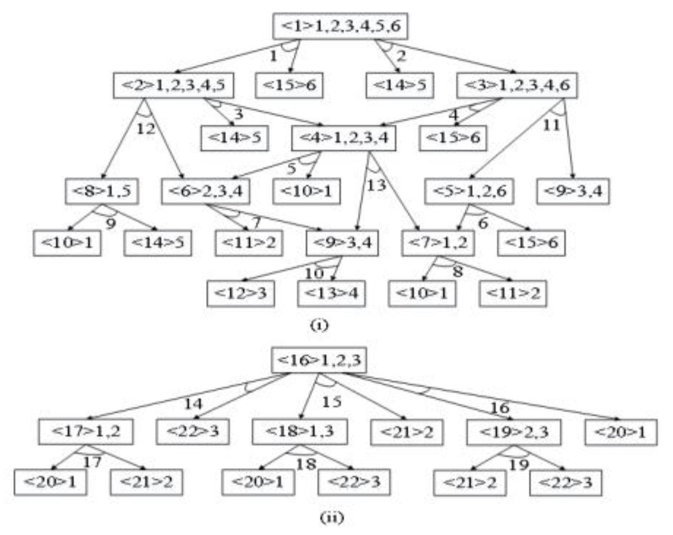
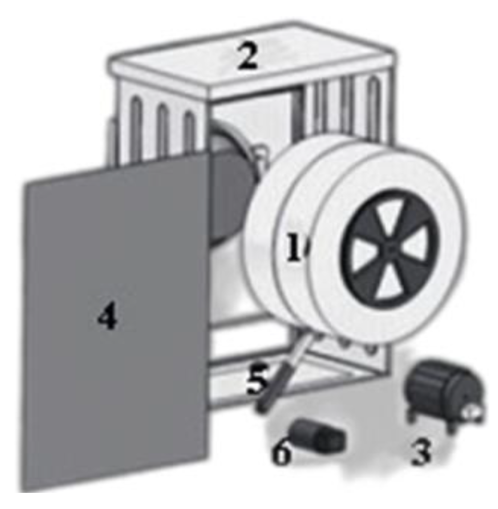
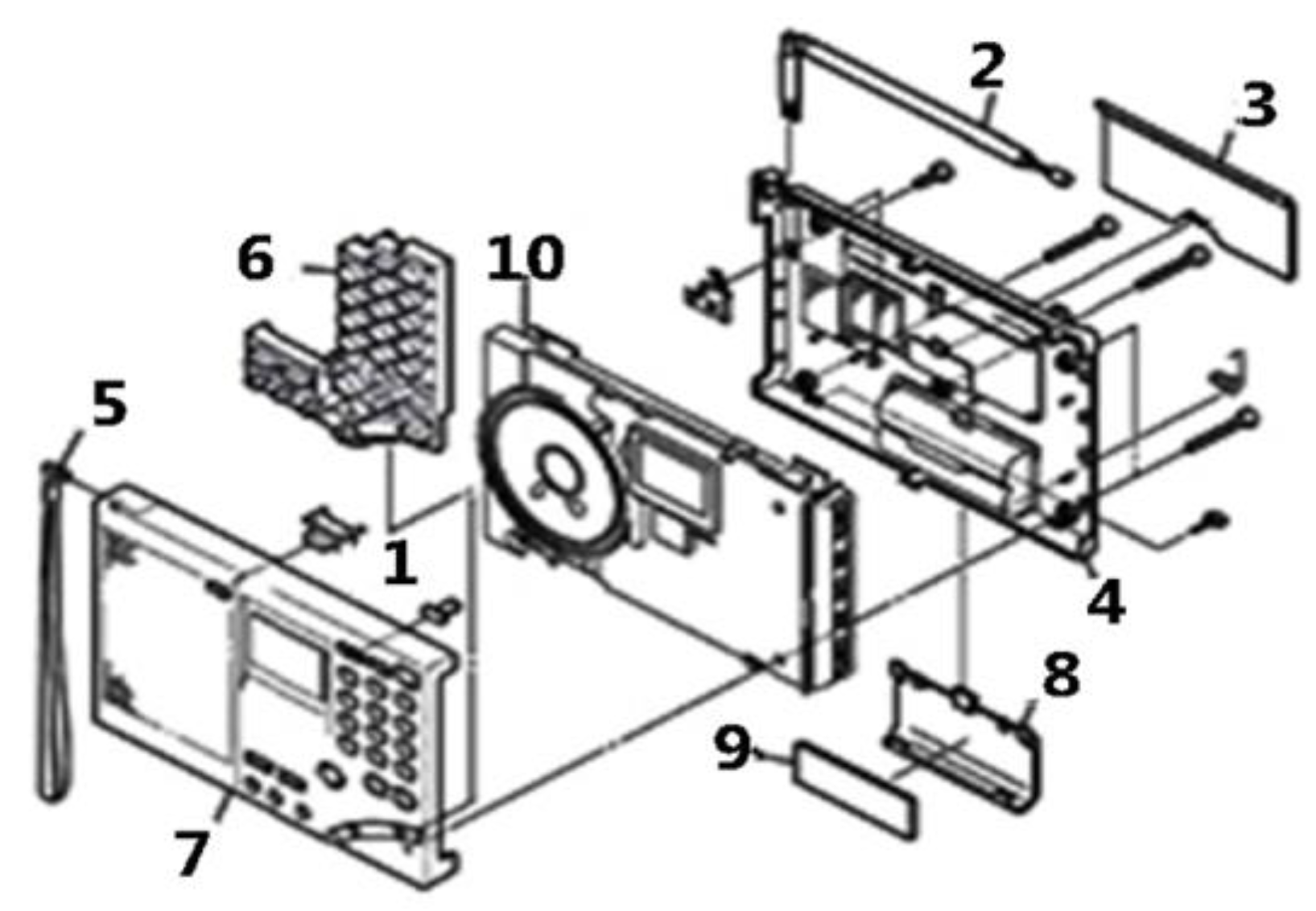
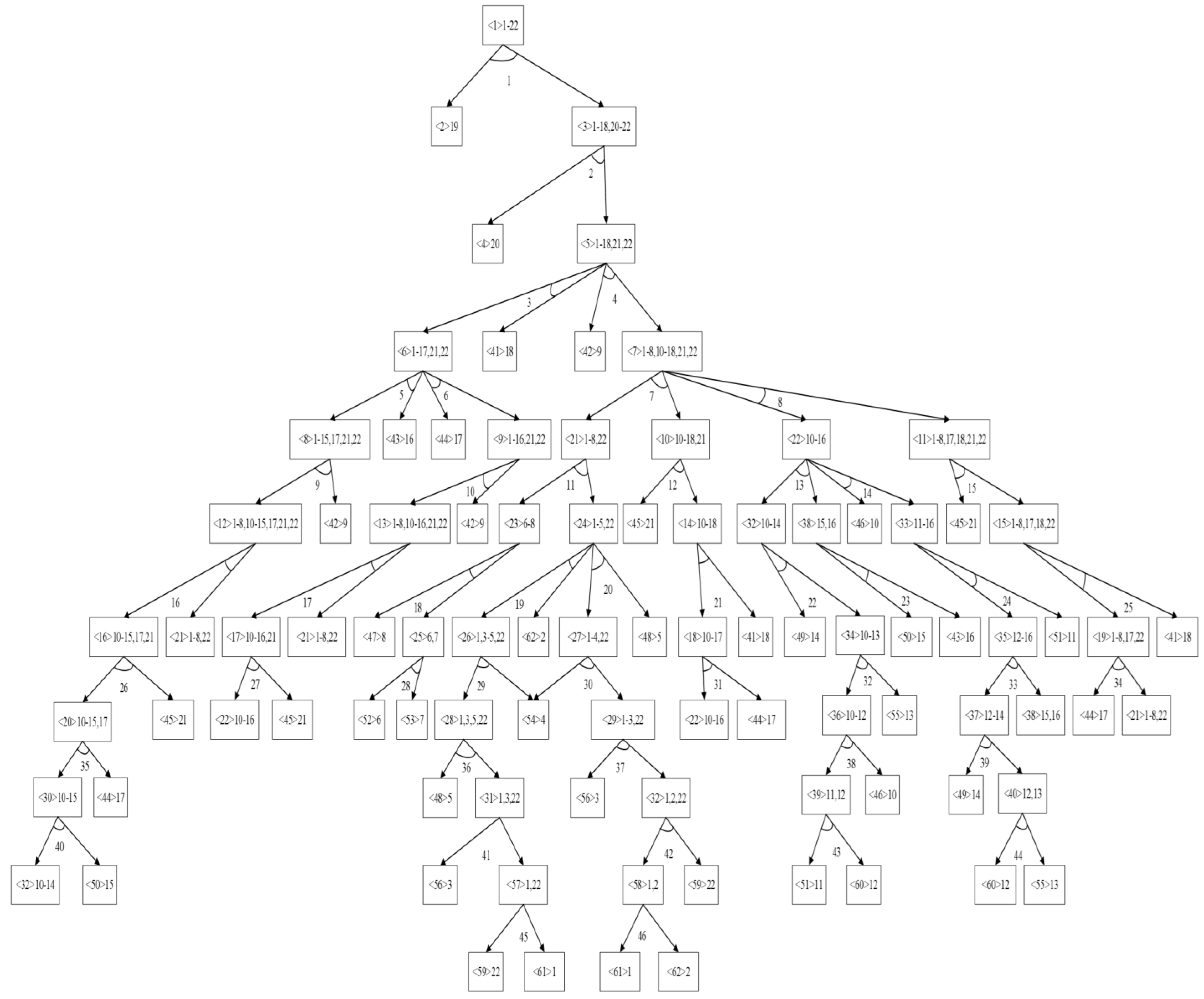
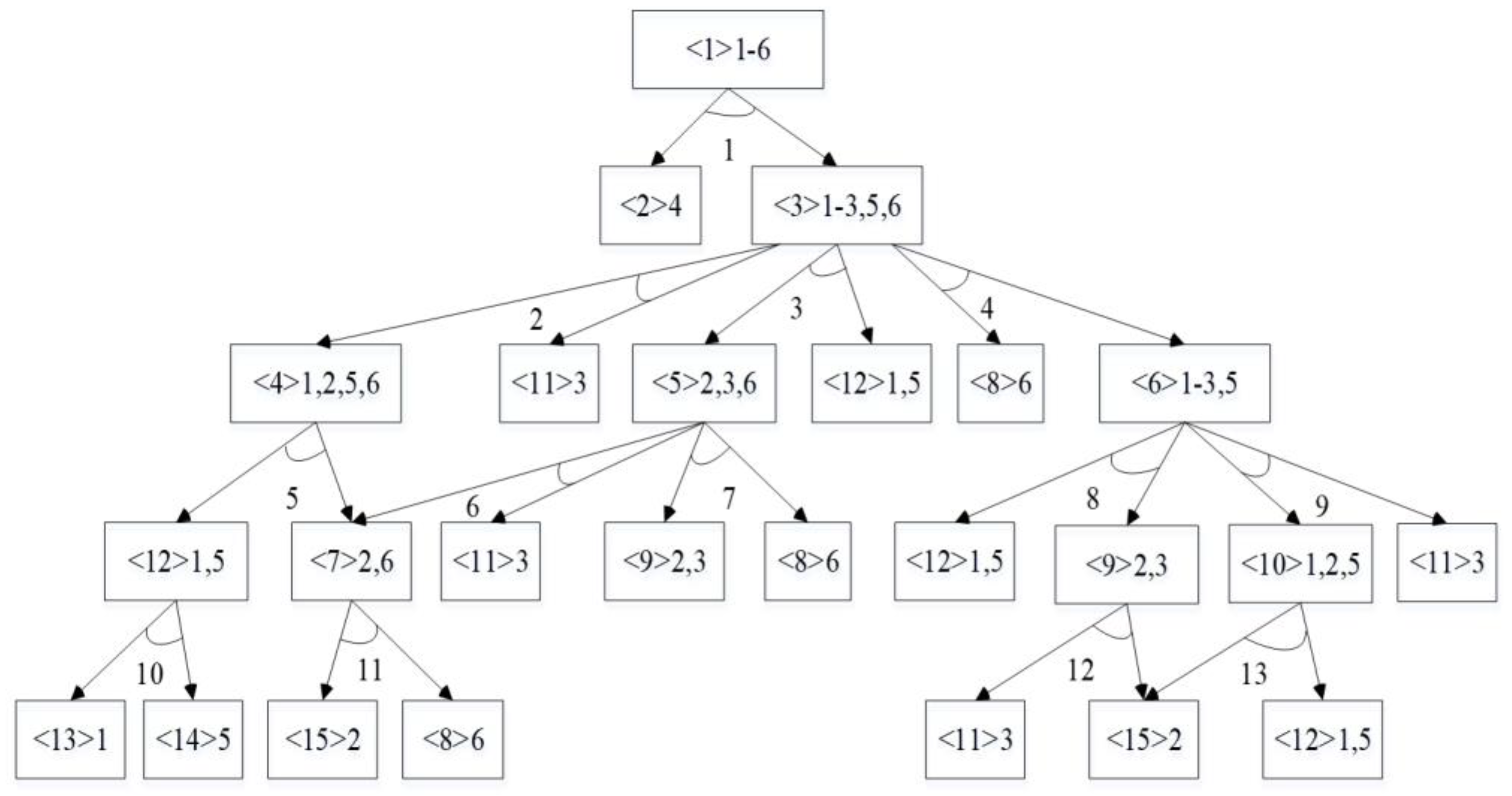
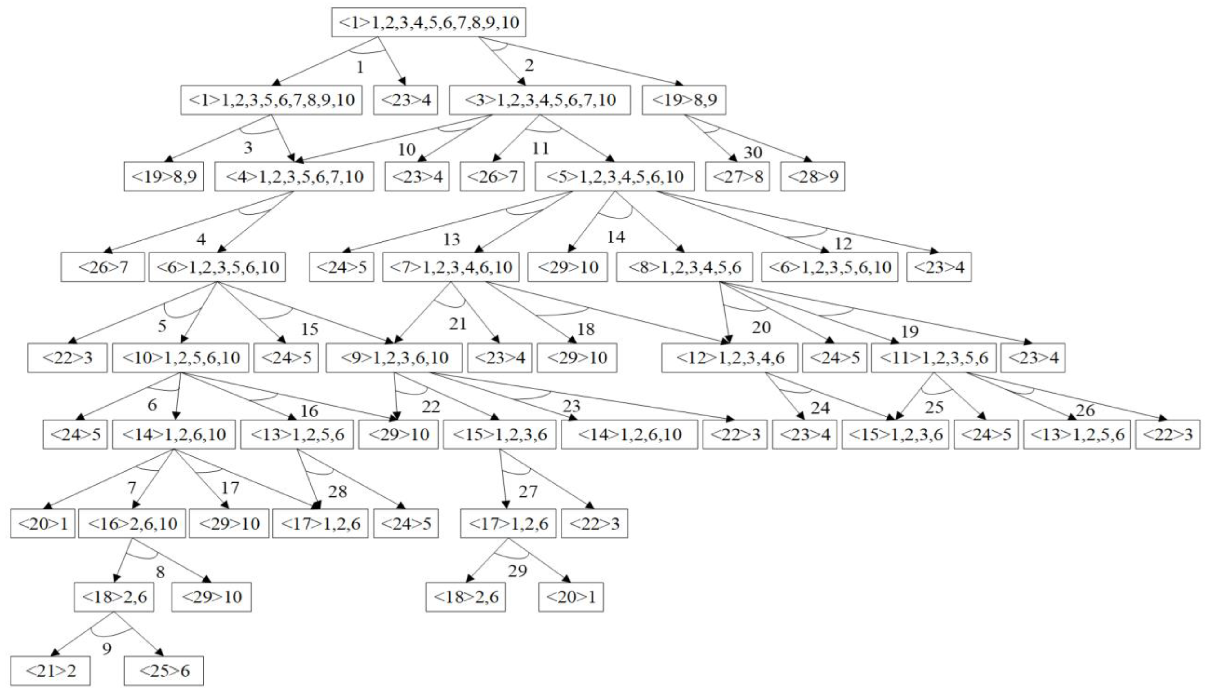
2.1. Subsection AND/OR Graph

An AND/OR graph is a graph model, which can express not only the precedence and conflict relationships between two disassembly operations but also the relationship between subassemblies/parts and disassembly operations. For example, Figure 1 shows the part structure schematic diagram of a ballpoint pen. Figure 2 shows the part structure schematic diagram of the lamp. Figure 3i,ii show the AND/OR graphs of the ballpoint pen and the lamp, respectively.
In Figure 3, the disassembly operations are represented with hyper-arc indices, 1 − J, where J is the total number of disassembly operations required to disassembly an EOL product. Nodes indicate subassemblies/parts with the index from <1> to <I>, where I is the number of all subassemblies/parts and components. Let subassembly a be a parent of subassembly b. If b is obtained by disassembling a, then b is called a child of a, where a, b∈{1,2, , I}. For example, in Figure 3i, subassembly <1> is the parent of <2> and <15>, while <2> is the child of <1>.
As shown in Figure 3, a disassembly operation disassembles a subassembly into two or more parts whose relationships are described by an “AND” relationship. An “OR” relationship denotes that a part has many ways to disassemble, but these ways cannot be performed simultaneously. For instance, parent subassembly <6> is disassembled into <9> and <11> by operation 7, and <8> is disassembled into <10> and <14> by operation 9. A parent subassembly may have more than one hyper-arc; for example, subassembly <2> can be disassembled via disassembly operations 3 or 12. Operations 3 and 12 form an OR relationship, which indicates that at most one of the two operations can be executed. According to the definition of an AND/OR graph and the logic of disassembly of a product, two matrices are proposed.
(1) Precedence matrix P = [ p j k ] is employed to describe the precedence and conflict relations of two disassembly operations, which is defined as
p j k = { 1 ,   if   operation   k   can   be   performed   after   opration   j ; 1 ,   if   operations   j   and   k   conflict   with   each   other ; 0 ,   otherwise .
Precedence matrix P of a multi-product instance for a ballpoint pen and lamp is given as
P = [ 0 1 1 1 1 1 1 1 1 1 1 1 1 0 0 0 0 0 0 1 0 1 1 1 1 1 1 1 1 1 1 1 0 0 0 0 0 0 0 1 0 1 1 1 1 1 1 1 1 1 1 0 0 0 0 0 0 1 0 1 0 1 1 1 1 1 1 1 1 1 0 0 0 0 0 0 0 0 0 0 0 1 1 1 1 1 1 1 1 0 0 0 0 0 0 1 0 1 1 1 0 1 1 1 0 0 1 1 0 0 0 0 0 0 0 0 0 0 0 1 0 1 0 1 1 0 1 0 0 0 0 0 0 0 0 0 0 1 0 1 0 1 0 0 1 0 0 0 0 0 0 0 0 1 1 1 1 1 0 1 0 0 1 0 1 0 0 0 0 0 0 0 0 0 0 0 0 0 0 0 0 0 0 0 0 0 0 0 0 0 1 0 1 1 1 1 1 1 1 1 0 1 1 0 0 0 0 0 0 0 1 1 1 1 1 1 1 1 1 1 0 1 0 0 0 0 0 0 0 0 0 0 1 1 1 1 1 1 1 1 0 0 0 0 0 0 0 0 0 0 0 0 0 0 0 0 0 0 0 0 0 1 1 1 1 1 0 0 0 0 0 0 0 0 0 0 0 0 0 1 0 1 1 1 1 0 0 0 0 0 0 0 0 0 0 0 0 0 1 1 0 1 1 1 0 0 0 0 0 0 0 0 0 0 0 0 0 0 1 1 0 1 1 0 0 0 0 0 0 0 0 0 0 0 0 0 1 0 1 1 0 1 0 0 0 0 0 0 0 0 0 0 0 0 0 1 1 0 1 1 0 ] .
(2) Disassembly-incidence matrix D = [ d i j ] expresses the corresponding relations between subassemblies/parts and disassembly operations, which is defined as
d i j = { 1 ,   if   subassembly   i   is   obtained   by   operation   j . 1 ,   if   subassembly   i   is   disassembled   via   operation   j . 0 ,   otherwise .
The disassembly-incidence matrix D of a multi-product instance for a ballpoint pen and lamp is as follows:
D = [ 1 1 0 0 0 0 0 0 0 0 0 0 0 0 0 0 0 0 0 1 0 1 0 0 0 0 0 0 0 0 1 0 0 0 0 0 0 0 0 1 0 1 0 0 0 0 0 0 1 0 0 0 0 0 0 0 0 0 0 1 1 1 0 0 0 0 0 0 0 1 0 0 0 0 0 0 0 0 0 0 0 1 0 0 0 0 1 0 0 0 0 0 0 0 0 0 0 0 0 1 0 1 0 0 0 0 1 0 0 0 0 0 0 0 0 0 0 0 0 1 0 1 0 0 0 0 1 0 0 0 0 0 0 0 0 0 0 0 0 0 0 1 0 0 1 0 0 0 0 0 0 0 0 0 0 0 0 0 1 0 0 1 1 0 1 0 0 0 0 0 0 0 0 0 0 1 0 0 1 1 0 0 0 0 0 0 0 0 0 0 0 0 0 0 0 0 1 1 0 0 0 0 0 0 0 0 0 0 0 0 0 0 0 0 0 0 0 0 1 0 0 0 0 0 0 0 0 0 0 0 0 0 0 0 0 0 0 1 0 0 0 0 0 0 0 0 0 0 1 1 0 0 0 0 0 1 0 0 0 0 0 0 0 0 0 0 1 0 0 1 0 1 0 0 0 0 0 0 0 0 0 0 0 0 0 0 0 0 0 0 0 0 0 0 0 0 0 0 1 1 1 0 0 0 0 0 0 0 0 0 0 0 0 0 0 0 0 1 0 0 1 0 0 0 0 0 0 0 0 0 0 0 0 0 0 0 0 1 0 0 1 0 0 0 0 0 0 0 0 0 0 0 0 0 0 0 0 1 0 0 1 0 0 0 0 0 0 0 0 0 0 0 0 0 0 0 1 1 1 0 0 0 0 0 0 0 0 0 0 0 0 0 0 0 1 0 1 0 1 0 0 0 0 0 0 0 0 0 0 0 0 0 1 0 0 0 1 1 ] .

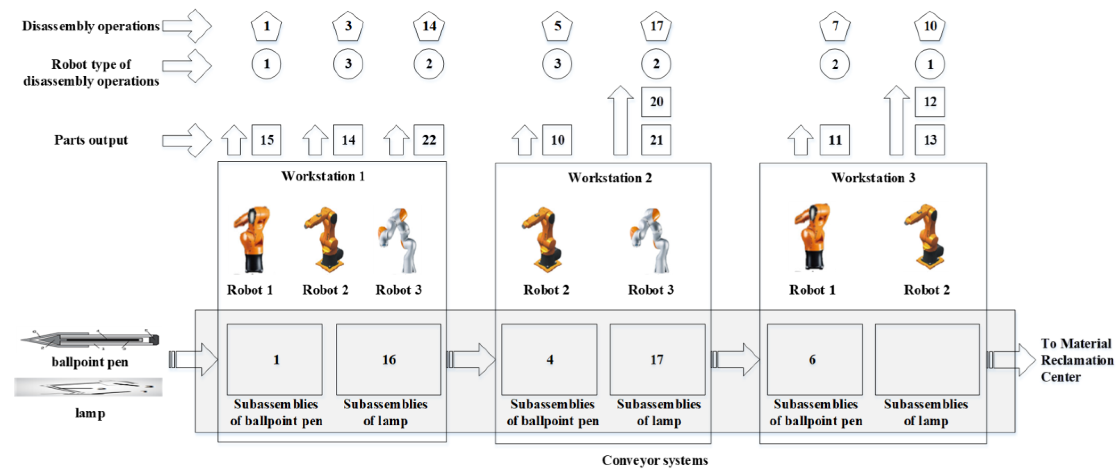
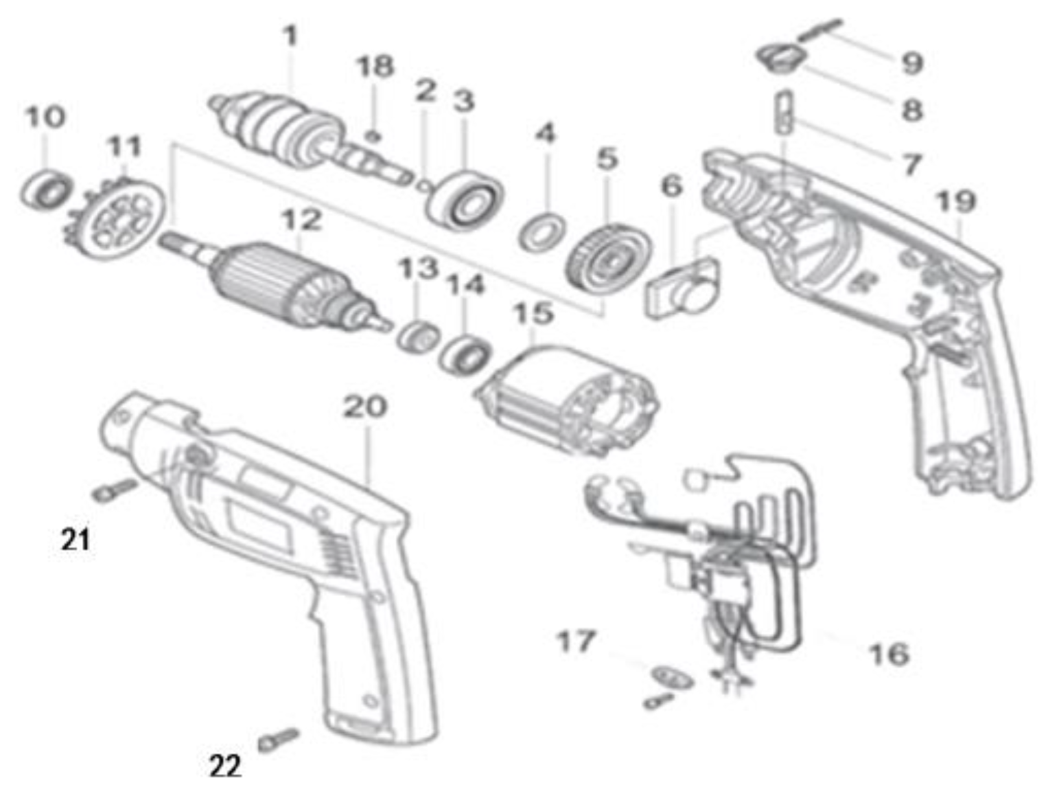
2.2. Robotic Disassembly Line

In Figure 3, 15 subassemblies/parts of a ballpoint pen correspond to 13 disassembly operations, and a lamp includes seven subassemblies/parts and six disassembly operations. In Figure 4, the number in the pentagon represents a disassembly operation, the number in the circle represents a type of robot that performs a disassembly operation, the number in the rectangle represents parts, and the number in the rectangle on the workstation represents the subassembly that is disassembled into subassemblies/parts. The disassembly operations are assigned to the workstation and then executed by the corresponding robot. As shown in Figure 3, disassembly operations 1–13 and subassemblies/parts 1–15 are related to the ballpoint pen, and disassembly operations 14–19 and subassemblies/parts 16–22 are related to the lamp. A robot in type i is denoted as ri. A feasible disassembly scheme contains a disassembly operation sequence 1, 3, 14, 5, 17, 7, and 10 and a robot type sequence 1, 3, 2, 3, 2, 2, and 1. Each disassembly operation in the disassembly operation sequence is mapped to the corresponding workstation according to a cycle time constraint. The robot types of each workstation are based on the robot type of the disassembly operation assigned to each workstation. For instance, disassembly operations 1, 3, and 14 are performed on the first workstation 1, and the robot types that perform these disassembly operations are 1, 3, and 2, respectively. Thus, r1, r2, and r3 are assigned to workstation 1. In addition, the parts 15, 14, 22, 10, 21, 20, 11, 12, and 13 are obtained by a feasible disassembly scheme where r1, r2, and r3 are assigned to workstation 1 to perform operations 1, 3, and 14, r2 and r3 are assigned to workstation 2 to perform operations 5 and 17, and r1 and r3 are assigned to workstation 3 to perform operations 7 and 10.

2.3. Mathematical Model

This paper makes the following assumptions to formulate a mathematical model of a stochastic MMRDP:
(1)
The average disassembly time and setup time of each disassembly operation of each type of robot are known.
(2)
The disassembly cost, setup cost, disassembly energy consumption, and setup energy consumption per unit time of each type of robot disassembly operation are given.
(3)
Only one robot is allowed to perform disassembly operations. Any robot can only handle one disassembly operation assigned to it at a time, and one disassembly operation can only be completed by one robot.
(4)
The supply of EOL products is unlimited.
(5)
AND/OR graphs of multiple EOL products to be disassembled are known.
Some notations and decision variables are listed below.

2.3.1. Notations

g —EOL product indices, g ∈{1, 2, …, G}, where G represents the number of disassembled products.
i—subassembly/part index, i∈{1, 2, …, N}, where N denotes the total number of subassemblies/parts of all products.
j, k—operation indices, j, k∈{0, 1, …, J}, where J means the total number of operations of all products, and 0 is a dummy operation.
l, m—workstation indices, l, m∈{1, 2, …, M}, where M is the number of workstations.
r —robot type index, r∈{1, 2, …, R}, where R denotes the number of robot types.
I g S —the start index set of subassembly/part of product g, I g S = { I 1 0 , , I g 0 , , I G 0 } , where I g 0 is the start index of subassembly/part of product g.
I g E { I 1 1 , , I g 1 , , I G 1 } , where I g 1 is the start index of subassembly/part of product g.
J g S —the start index set of tasks of product g, J g S = { J 1 0 , , J g 0 , , J G 0 } , where J g 0 is the start index of tasks of product g.
J g E —the end index set of tasks of product g, J g E = { J 1 1 , , J g 1 , , J G 1 } , where J g 1 is the end index of tasks of product g.
t j r —disassembly time for operation j by robot r.
t j k r —setup time of performing operation k which is performed immediately after operation j by robot r.
e j r —energy consumption per unit of time of robot r performing operation j.
e j k r —setup energy consumption per unit of time in performing operation k performed immediately after operation j by robot r.
el—energy consumption per unit of time during the l-th workstation operation.
c j r —cost per unit of time of robot r performing operation j.
c j k r —setup cost per unit of time in performing operation k performed immediately after operation j by robot r.
cl—cost per unit of time during the l-th workstation operation.
v i —reuse value of subassembly/part i.
Tl—cycle time of the l-th workstation.
q j k r —failure probability of operation k performed immediately after operation j in product g by robot r.
θ—preset minimum probability value
—maximum failure cost of a disassembly process.
P—multiple products precedence matrix
D—multiple products disassembly-incidence matrix
p j k —an element in the j -th row and k -th column of P.
d i j —an element in the i -th row and j -th column of D.
Notice that t j r g , t j k r g , and t j k r g φ are random variables with normal distribution.

2.3.2. Decision Variables

x j r —if operation j is performed by robot r, x j r = 1 ; otherwise, x j r = 0 .
y j k r —if operation k is performed immediately after operation j by robot r, y j k r = 1 ; otherwise, y j k r = 0 .
z j r l —if operation j is performed by robot r and assigned to the l-th workstation, z j r l = 1 ; otherwise, z j r l = 0 .
ul—if the l-th workstation is used, ul = 1; otherwise, ul = 1.
On the basis of AND/OR graphs and relationship matrices, multiple EOL products to be disassembled can be mathematically described. The mathematical model is given below.
The expected maximal disassembly profit is the total profit obtained from disassembly minus total disassembly cost in the disassembly process. As shown in Equation (1), the latter consists of three main parts, i.e., the cost of disassembly operations, the setup cost of adjacent operations, and the cost of workstations.
max f 1 = E ( g = 1 G j = J g 0 J g 1 i = I g 0 I g 1 r = 1 R d i j v i x j r g = 1 G j = J g 0 J g 1 r = 1 R t j r c j r x j r g = 1 G φ = 1 G j = J g 0 J g 1 k = J φ 0 J φ 1 r = 1 R t j k r c j k r y j k r l = 1 M T l c l u l ) .
The expected minimal energy consumption mainly takes into account three aspects of energy consumption, i.e., the total energy consumption of disassembly operations, the total setup energy consumption of adjacent operations, and the energy consumption of workstations, as shown in Equation (2).
min f 2 = E ( g = 1 G j = J g 0 J g 1 r = 1 R t j r e j r x j r + g = 1 G φ = 1 G j = J g 0 J g 1 k = J φ 0 J φ 1 r = 1 R t j k r e j k r y j k r + l = 1 M T l e l u l ) .
The expected maximal balancing rate is equal to the average of the total operating time divided by the total cycle time of the switched-on workstations, as shown in Equation (3).
max f 3 = E ( ( g = 1 G j = J g 0 J g 1 r = 1 R t j r x j r + g = 1 G φ = 1 G j = J g 0 J g 1 k = J φ 0 J φ 1 r = 1 R t j k r y j k r ) / l = 1 M T l u l ) .  
The fact that each product is disassembled by at least one disassembly operation excluding operation 0 is constrained by Equation (4).
j = J g 0 J g 1 r = 1 R x j r 1 , g = 1 , 2 , , G .      
Each disassembly operation in multiple products should be performed at most once, which is constrained by Equation (5).
r = 1 R x k r = j = J g 0 J g 1 r = 1 R y j k r , g = 1 , 2 , , G , k = 1 , 2 , , J .    
Each disassembly operation of any product can only be assigned to one workstation and can only be performed by one robot, which is constrained by Equation (6).
r = 1 R x j r = l = 1 M r = 1 R z j r l , g = 1 , 2 , , G , j = 1 , 2 , , J .  
Each switched-on workstation must be assigned at least one operation, which is constrained by Equation (7).
g = 1 G j = J g 0 J g 1 r = 1 R x j r z j r l   1 ,   l = 1 , 2 , , M .  
To ensure that a feasible disassembly sequence of multiple products satisfies precedence constraint, this paper explicitly defines
l = 1 M r = 1 R l z j r l m = 1 M r = 1 R m z k r m , g = 1 , 2 , , G , p j k = 1 .
To ensure that a feasible disassembly sequence of multiple products satisfies conflict constraint, this paper proposes Equation (9).
l = 1 M r = 1 R z j r l + l = 1 M r = 1 R z k r l 1 ,   g = 1 , 2 , , G , p j k = 1 .
The operation time of all workstations used is no more than the disassembly line total cycle time, represented by Equation (10).
g = 1 G j = J g 0 J g 1 r = 1 R t j r x j r + g = 1 G φ = 1 G j = J g 0 J g 1 k = J φ 0 J φ 1 r = 1 R t j k r y j k r l = 1 M T l u l ,   l = 1 , 2 , , M .  
The probability for the failure cost of a disassembly process being less than or equal to its maximum failure cost is greater than a preset value θ > 0, required by Equation (11).
𝒫 { g = 1 G φ = 1 G j = J g 0 J g 1 k = J φ 0 J φ 1 r = 1 R ( t k r c k r x k r + t j k r c j k r y j k r ) q j k r < } θ .
The range of decision variables is given by Equation (12).
x j r , y j k r , z j r l , u l { 0 , 1 } , g , φ = 1 , 2 , , G ,   j , k = 1 , 2 , , J , l = 1 , 2 , , M ,   r   = 1 ,   2 ,   ,   R .

3. Proposed Algorithm

3.1. Base Brainstorming Optimization Algorithm

Brainstorming conference is the process of discussing solutions to difficult problems. The brainstorming optimization (BSO) algorithm is inspired by this feature of group discussion and speaking freely [21]. There are three roles involved in a brainstorming conference, i.e., several owners of problems to be solved, and a group of members with different backgrounds. Since practical experience and ways of thinking are different, for the same problem, they can put forward different solutions. The conference stipulates that the host presides over and urges the team members to generate as many ideas as possible, but the host does not participate in an idea generation process. In addition, four rules are given as follows:
(1) Any idea is meaningful. All ideas, good or bad, cannot be judged until the end of a brainstorming process.
(2) Brainstorming team members should be unreserved, and any ideas generated in their minds should be shared and studied.
(3) Many new ideas are generated by associating with the existing ideas.
(4) Many new ideas are generated as possible and then choose from abundant ideas to get excellent solutions.
In BSO, each solution is represented separately by an individual idea. In a human brainstorming conference, each idea is inspired by other individual ideas and becomes more mature. The same is true in BSO, where one individual is updated through individual evolution and fusion. The algorithm consists of three strategies: solution clustering, new individual generation, and solution selection.
The MMRDP is a multi-objective, stochastic, and discrete optimization problem. However, the basic BSO algorithm was originally proposed to solve single-objective and continuous optimization problems. Therefore, some special strategies need to be designed according to the characteristics of MMRDP. This paper proposes a PIMBO algorithm incorporated with a stochastic simulation approach.

3.2. Encoding

A solution is represented by a triple-vector list designed for this work, i.e., π = (π1, π2, π3), where π1 = (o1, o2, …, oJ) is an integer string. It denotes a disassembly operation sequence, where oj indicates an operation index of the j-th disassembly operation, and J is the maximum index of disassembly operations for multiple products to be disassembled. π2 = (x1, x2, …, xJ) is a binary vector with J binary values indicating whether the disassembly operation at the corresponding position is performed. If xj = 1, the operation oj in π1 is performed; otherwise, oj is not performed. π3 = (r1, r2, …, rJ) represents a robot type sequence, whose element is an integer between 1 and R and corresponds to the robot type performing a disassembly operation.

3.3. Population Initialization
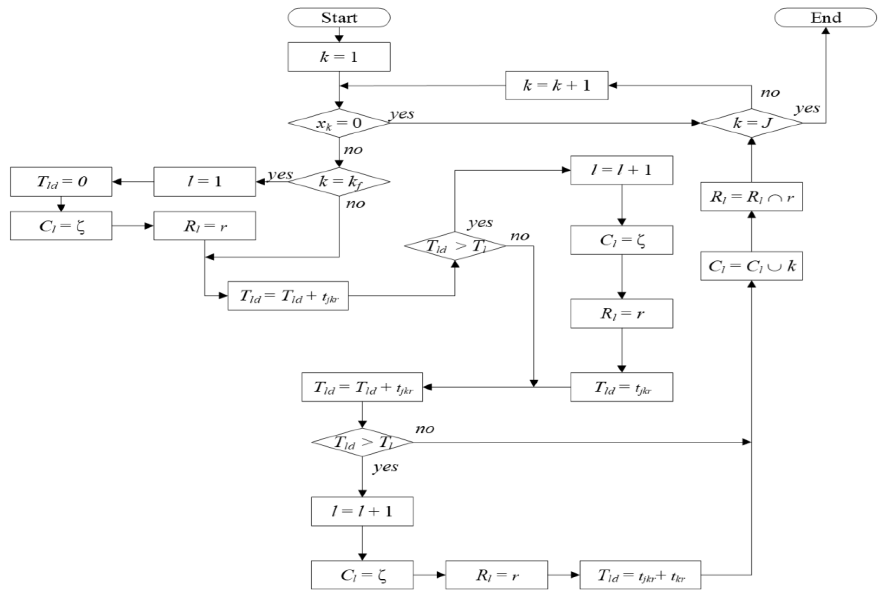
The key to solve the proposed problem is to design a reasonable population initialization strategy according to the above encoding rules. The proposed algorithm employes the random initialization method of MMRDP solutions to generate diversified initial population in the searching space. Notice that a solution may be infeasible in the case that it disobeys precedence and conflict constraint conditions. In this work, an adjustment approach is developed to initialize individuals so that each solution becomes feasible. The following steps detail its adjustment process:
Step 1: Randomly generate π, i.e., π1, π2, and π3.
Step 2: Adjust the disassembly operation sequence in π1 according to the rules specified in matrix P to meet the precedence relationship between disassembly operations of multiple products. It is required to traverse the whole disassembly operation sequence π1. If the disassembly operation oj is after ok, but pjk = 1 in matrix P, which is a contradiction, then oj and ok need to be interchanged in the correct order, and rj and rk are swapped at the same time; otherwise, it indicates that operation j and k are in accordance with the disassembly sequence. Lastly, check the next disassembly operation.
Step 3: In order to make the disassembly proceed smoothly, the first disassembly operation must be performed. Hence, if operation oj in π1 is the first disassembly operation of a product but xj = 0 in π2, then adjust xj to 1; otherwise, go to Step 4.
Step 4: Adjust the binary values in π2 based on matrix P to meet the precedence relationship between disassembly operations of the same product. It is required to traverse the whole binary vector π2. If xk = 1 and pjk = 1 in matrix P, then xj is set to 1.
Step 5: Adjust the binary values in π2 based on P to remove the conflict relationship between operations of the same product to be disassembled. The above process needs to traverse the entire vector π2. If xj = 1 and pjk = −1, then xk = 0.
After completing the strategy steps described above, an initial population set which contains Q solutions (individuals) is obtained.

3.4. Decoding

The decoding task is completed by assigning the selected disassembly operations and the robot to each corresponding workstation. Therefore, a disassembly operation and the robot performing it should be assigned to the same workstation at the same time. Moreover, a cycle time constraint needs to be satisfied when assigning disassembly operations to workstations. Figure A1 of Appendix A.1 shows the decoding procedure, the detailed steps of which are as follows:
Step 1: Set disassembly operation k = 1.
Step 2: Verify that the disassembly operation k is performed. If xk = 1 and k = kf where kf is the first disassembly operation in the whole disassembly sequence, open the l-th workstation; the processing time of the l-th workstation Tld is set to 0, the disassembly operation set Cl in the l-th workstation is set to ζ, where ζ represents an empty set, and the robot set Rl of the l-th workstation is set to r, where r means a type of robot performing disassembly operation k. If xk = 1 and kkf, perform disassembly operation k, followed by Step 3; otherwise, perform Step 8.
Step 3: Set T l d = T l d + t j k r , and determine the relationship between the cycle time Tl and the current processing time of the l-th workstation Tld. If Tld > Tl, then perform Step 4; otherwise, perform Step 5.
Step 4: Start the next workstation; let l = l + 1, Cl = ζ, Rl = r, and T l d = t j k r .
Step 5: Set T l d = T l d + t k r , and determine the relationship between Tl and Tld. If Tld > Tl, then perform Step 6; otherwise, perform Step 7.
Step 6: Start the next workstation; let l = l + 1, Cl = ζ, Rl = r, and T l d = t j k r + t k r .
Step 7: Disassembly operation k is assigned to the l-th workstation; then, update Cl and Rl, and let Cl = Clk and Rl = Rlr.
Step 8: If kJ, then set k = k + 1, and repeat Steps 2–7. Otherwise, output a feasible solution.

3.5. Objective Function Evaluation

After performing the relevant operations in Section 3.2, Section 3.3 and Section 3.4, many feasible solutions of MMRDP are generated, and the next step is to evaluate them. The MMRDP is different from a deterministic optimization problem. The objective function values of the latter can be straightforwardly calculated according to its objective functions and constraints. In the MMRDP, the disassembly and setup times of the products are randomly generated, and the objective functions in Equations (1)–(3) are expressed as their expected values. They cannot be calculated directly as deterministic optimization problems. Hence, Monte Carlo simulation is used to successfully solve the above problems [31].
Let π be a solution; Γ denotes the number of samples equaling 10. This paper adopts the following steps to evaluate the objective function values and feasibility of π . It should be noted that since the objective functions f 1 and f 3 are to find their maximum values, the values of the objective functions f 1 and f 3 obtained are multiplied by −1 to facilitate the comparison of the quality of the solutions later.
Step 1: f 1 ( π ) 0 , f 2 ( π ) 0 , f 3 ( π ) 0 , f c ( π ) 0 , and Γ 10 .
Step 2: Generate δ samples; each sample ρ δ is a sample of disassembly and setup times produced from their normal distributions, δ = 1 , 2 , , Γ .
Step 3: Calculate the disassembly profit f 1 δ ( π ) , energy consumption f 2 δ ( π ) , balancing rate f 3 δ ( π ) , and disassembly failure cost f c δ ( π ) , where δ = 1 , 2 , , Γ .
Step 4: Sort the disassembly failure cost f c δ ( π ) of all samples in ascending order; let δ be equal to θ · Γ . If f c δ ( π ) < , π is feasible and f c ( π ) f c δ ( π ) , then go to Step 5. Otherwise, π is infeasible, where f 1 ( π ) , f 2 ( π ) , and f 3 ( π ) are equal to larger integers; then, go to Step 6.
Step 5: Approximate the expected disassembly profit f 1 ( π ) , energy consumption f 2 ( π ) , and balancing rate f 3 ( π ) as follows:
f 1 ( π ) 1 × δ = 1 Γ f 1 δ ( π ) Γ .    
f 2 ( π ) δ = 1 Γ f 2 δ ( π ) Γ .
f 3 ( π ) 1 × δ = 1 Γ f 3 δ ( π ) Γ .  
Step 6: Return f 1 ( π ) , f 2 ( π ) , and f 3 ( π ) as the approximated values of Equations (1), (2), and (3).

3.6. Multi-Objective Processing Method

In order to distinguish the advantages and disadvantages of the obtained solutions, this work uses Pareto dominance relationship. The process of comparison is the decision-making process of a choice of solutions.
An external archive A is constructed to store the obtained nondominated solutions. First, it is updated by using all newly generated solutions based on the Pareto rule. After each iteration is finished, A is updated by using the current population based on the Pareto rule to ensure that all nondominated solutions in A are always the current global nondominated solutions.

3.7. Pareto-Based Clustering

During the clustering stage, this work uses the fast nondominated sorting approach proposed in [24]. The individuals are ranked according to the Pareto rule, and then the individuals of the same rank are classified into the same cluster. The k-means clustering constantly calculates the new clustering center after adjusting the sample classification, thus resulting in a large amount of calculation. However, the Pareto-based clustering algorithm reduces the computational complexity, and the number of clusters needs not to be predetermined. The pseudo-code of Pareto-based clustering is shown in Algorithm A1 of Appendix A.2.

3.8. New Individual Generation

The pseudo-code of new individual generation is shown in Algorithm A2 of Appendix A.3, where X denotes the set of new individuals, pc is the probability of replacing a cluster center, pg is the probability that a new individual is generated from one subcluster, po is the probability that a new individual is generated concerning a subcluster center, and pt is the probability that a new individual is generated by combining with two subcluster centers.
In the original BSO, when a random number ϑg is less than pg, only one individual contributes to generate a new individual. This paper combines the center of the first cluster with the current selected individual to generate a new individual, which improves the convergence speed of the algorithm. Moreover, this paper adopts a precedence preserving crossover (PPX) [32] operator and a position-based mutation (PBM) [27] operator to generate a new individual.

3.9. Selection Operator

The selection algorithm is used to retain the solutions with better quality among all the solutions found so far. To accelerate the convergence of the algorithm, the first Q individuals in the combination of and A are chosen as the next population by using rank and crowding distance approaches in [24].

3.10. Procedure of PIMBO

The procedure of PIMBO is summarized as follows:
Firstly, all parameters involved in the algorithm are set initially and then an initial population is generated and evaluated.
Secondly, with the given termination condition, the algorithm enters the following loop: the Pareto-based clustering, new individual generation, and selection are performed repeatedly until a given termination condition is reached.
Lastly, all solutions in A are output.
In this paper, the iterations of the PIMBO and its comparison algorithm are determined by the fitness value. Before the PIMBO starts to iterate, the fitness value is equal to 0. When evaluating a new individual, the fitness value is increased by 1 until the current fitness value f v reaches the preset total fitness value f t v ; then, the algorithm stops the iteration. Algorithm 1 gives the pseudo-code of PIMBO.
Algorithm 1: PIMBO
Input: pc, pg, po, pt, | |, ftv,cl,Tl,θ, R, crossover probability, and mutation probability.
Output: all solutions in A .
Begin
   Set algorithm parameters.
   Initialize population as shown in Section 3.2 and Section 3.3.
   Perform decoding process as shown in Section 3.4.
   Evaluate solutions as shown in Section 3.5.
   while ( f v < f t v )
      Perform Pareto-based clustering as shown in Section 3.7.
      Execute new individual generation as shown in Section 3.8.
      Construct next population as shown in Section 3.9.
   end while
      Output all solutions in A .
End.

4. Experiments

To test the performance of PIMBO in handling the considered problem, this work conducts experiments by adopting the set of EOL products given in [4,12,33]. Additionally, MDGWO [27], MOABC [28], NSGAII [24], and MOEAD [29] are compared. They have shown excellent performance in solving various optimization problems and have been used as a benchmark for comparison by many scholars and practitioners [34]. Accordingly, this paper chooses MDGWO, MOABC, NSGAII, and MOEAD as the peer methods. In this work, the position-based crossover and position-based mutation operations are adopted by these algorithms to generate new solutions.

4.1. Test Instance Generation

In order to have sufficient experimental data, this work collects a large amount of product data in the literature as examples: ballpoint pen (BP) [4], hammer drill (HD) [12], washing machine (WM) [35], and radio set (RS) [4]. A BP contains 15 subassemblies/parts, and 13 disassembly operations are needed to disassemble it. An HD includes 62 subassemblies/parts, and 46 disassembly operations should be adopted to disassemble it. A WM contains 15 subassemblies/parts, and 13 disassembly operations are used to disassemble it. There are 29 subassemblies/parts in an RS, and 30 disassembly operations are needed to disassemble it. Their schematic diagrams and AND/OR graphs are shown in Figure A2, Figure A3, Figure A4, Figure A5, Figure A6 and Figure A7 of Appendix A.4. By adopting BP, HD, WM, and RS, 10 test instances of small and medium-sized disassembly tasks are generated, and each instance contains multiple disassembled products. Their corresponding relationships are given in Table 1, where represents the maximum failure cost of all disassembly operations performed in each case.

4.2. Performance Metrics

This work utilizes three metrics to examine the results obtained by PIMBO and its peers to verify the performance of PIMBO algorithm, i.e., C-metric [29], IGD metric [35], and hypervolume metric [35]. The C-metric can measure the dominated percentage of two solution sets.
IGD calculates the average distance of the obtained solutions to their nearest solutions in an optimal solution set. A smaller IGD of a solution set denotes a better approximation and distribution. Notice that this work cannot acquire an optimal solution set for the proposed MMRDP beforehand. Thus, an optimal solution set is composed of all solution sets obtained by PIMBO and its peers.
Hypervolume can comprehensively evaluate the convergence and distribution of nondominated solution sets. It focuses on computing the volume as constructed by the obtained solutions and the reference point. A bigger hypervolume of a solution set denotes a better approximation and distribution. It is worth noting that, when calculating the hypervolume of the solutions, this work multiplies the first objective value and the third objective value of all solutions by −1 since the first and third objective functions in the investigated problem are to maximize the profit and balancing rate, respectively.
PIMBO and its comparison algorithms were used to solve each instance 20 times, and then these solutions were used to calculate the average value of the three metrics of each algorithm. Additionally, this paper analyzes the experimental results by employing a one-tailed t -test [36] with 38 degrees of freedom at a 0.05 level of significance. In the following analysis of experimental results, we use the symbols “+”, “−”, or “~” to illustrate the comparison results between P and other algorithms The symbol “+” means that PIMBO is significantly better than its peer methods, The symbol “−” indicates that PIMOB is significantly worse than its peers, while “~” denotes that PIMBO is statistically equivalent to its peers.

4.3. Parameter Setting

In order to improve the performance of the proposed PIMBO algorithm, the parameters are set as follows: pc = 0.2, pg = 0.8, po = 0.4, and pt = 0.5 [37]. The parameters used in all algorithms are set as follows: population size | | = 120, crossover probability = 1, mutation probability = 0.3, and total fitness value ftv = 2000. The parameters involved in the objective functions are set as follows: cl = 0.03, el = 0.05, Tl = 50, θ = 0.90, and R = 3 [6,14]. To avoid chance, each algorithm is executed 20 times independently, and their average running time in each instance is shown in Table 2. This work concludes that PIMBO could find a promising solution set in less time.

4.4. Case Analyzes

Table 3 shows 10 nondominated solutions generated by solving instance 2 through PIMBO, where f1, f2, f3, fc, and rs denote profit, energy consumption, balancing rate, failure cost, and robot type set assigned to switched-on workstations, respectively. According to the previous description, BP has 13 disassembly operations, and HD has 46 disassembly operations. Therefore, disassembly operations 1–13 in these solutions represent the disassembly operations of BP, and 14–59 represent the disassembly operations of HD. In the first solution, disassembly operations 2 and 11 are from BP, and disassembly operations 14, 15, 17, 20, 24, 32, 42, 49, and 31 are from HD. A robot in type i is denoted as ri. Disassembly operations 14, 15, and 17 are performed by r1 and r2 in the first workstation, disassembly operations 2, 20, 11, and 24 are performed by r1 and r3 in the second workstation, and disassembly operations 32, 42, 49, and 31 are performed by r3 in the third workstation. The profit, energy consumption, balancing rate, and failure cost are 978.94, 998.13, 0.9459, and 63.03, respectively. Therefore, this solution to the considered problem in this research is satisfactory.

4.5. Results

In this section, the five algorithms are used to calculate the 10 test instances provided, and the C-metric, IGD metric, and hypervolume metric are employed to analyze the previous calculation results. In Table 4, Table 5 and Table 6, the symbols “t-te”, “m”, and “v” represent the “t-test”, “mean”, and “variance”, respectively.
Table 4 gives the comparative experimental results of five algorithms with respect to the C-metric, where the symbols A, B, E, U, and V denote PIMBO, MDGWO, MOABC, NSGAII, and MOEAD, respectively. Analyzing the experimental results of this metric, we can conclude that all solutions obtained by PIMBO could dominate those found by MDGWO, MOABC, and NSGAII since C(A, B), C(A, E), and C(A, U) were greater than C(B, A), C(E, A), and C(U, A), respectively. However, there are three instances where more solutions obtained by PIMBO could dominate those acquired by MOEAD. The average values of C(A, B), C(B, A), C(A, E), C(E, A), C(A, U), C(U, A), C(A, V), and C(V, A) were 0.7332, 0.1002, 0.7879, 0.0585, 0.9057, 0.0155, 0.1956, and 0.3362, respectively. These results confirm that PIMBO outperformed MDGWO, MOABC, and NSGAII, whereas it was inferior to MOEAD for coping with the concerned problem.
Table 5 reveals the comparative experimental results of the five algorithms according to the IGD metric. By analyzing the comparison results of this metric, we can clearly conclude that PIMBO performed better than MDGWO, MOABC, NSGAII, and MOEAD for solving the concerned problem since the IGD values of PIMBO were smaller than those of MDGWO, MOABC, NSGAII, and MOEAD in most instances. The average values of the five algorithms for 10 instances were 0.1338, 0.2105, 0.2115, 0.2599, and 0.1617, respectively. According to the analysis of the above experimental results, the algorithm designed in this paper could obtain a nondominated solution set with fast convergence speed and rich diversity when solving the concerned MMRDP.
In order to reveal the performance of PIMBO and its peers more comprehensively, the hypervolume metric was adopted to analyze the experimental results in Table 6. It can be found that the hypervolume values obtained by PIMBO were bigger than those of NSGAII in all instances. There were seven instances where the hypervolume values obtained by PIMBO were bigger than those of MDGWO and MOABC, and there were six instances where the hypervolume values obtained by PIMBO were bigger than those of MOEAD. Through more detailed calculation, the average values of the five algorithms for 10 instances were 0.4613, 0.4228, 0.4352, 0.3737, and 0.4477, respectively. Hence, this demonstrates that, compared with MDGWO, MOABC NSGAII, and MOEAD, PIMBO provided more uniformly distributed solutions in the solution set when solving MMRDP. In order to further and more visually describe the experimental results, this paper presents the boxplots of experimental results of the five algorithms for 10 instances in terms of the IGD metric and hypervolume metric in Figure A5 and Figure A6 of Appendix A.4, respectively. In Figure A5, “HV” denotes the hypervolume value. From the experimental results and Figure A5 and Figure A6, this work can conclude that PIMBO had better performance than MDGWO, MOABC, NSGAII, and MOEAD in dealing with the proposed problem.

5. Conclusions

This work introduced the MMRDP in an uncertain environment with objectives of maximization of profit and balancing rate, as well as minimization of energy consumption. A detailed and complete mathematical model was developed to display the MMRDP. Then, an improved PIMBO algorithm was formulated by incorporating a stochastic simulation approach to solve the MMRDP. Through the comparison of multiple groups of experiments, the proposed algorithm was shown to have excellent phenotype under the measurement of the selected metrics The experimental results can assist producers to make more diversified decision plans.
For future work, we plan to strive in two directions: (1) to consider more practical issues based on this model such as U-type, circular type, and parallel disassembly lines [38,39]; (2) to design much better intelligent algorithms to deal with highly complex optimization problems [40,41,42,43,44,45].

Author Contributions

Formal analysis, Z.L.; Data curation, X.G. and X.L.; Writing—original draft, G.X.; Writing—review & editing, Z.Z.; Supervision- data accuracy, L.Q. All authors have read and agreed to the published version of the manuscript.

Funding

This work is partially supported by the Guangzhou Innovation and Entrepreneurship Leading Team Project Funding under Grant No. 202009020008.

Data Availability Statement

Conflicts of Interest

The authors declare no conflict of interest.

Appendix A

Appendix A.1. Decoding Procedure

Figure A1. The flowchart of decoding.
Mathematics 11 01557 g0a1

Appendix A.2. Clustering

The pseudo-code of Pareto-based clustering is shown in Algorithm A1, where p represents a subcluster in cluster , and τ denotes the rank level of individuals.
Algorithm A1: Pareto-Based Clustering
Input: all individuals in population .
Output: the cluster .
Begin
Initialize two sets δ and p . Define an integer r to represent the rank level of an individual. δ , p , τ  1. Rank individuals in δ according to Pareto rule.
      while (δ )
         for ( i Q to 1 ) do
            Choose all individuals of the same rank level r from δ.
            Move them to p and delete it from δ.
         end for
        Add p to and the first individual in p as center.
         p . r++.
        end while
End

Appendix A.3. New Individual Generation

Algorithm A2: New Individual Generation
Input: Q individuals in population , the cluster .
Output:   X , A .
Begin
Randomly generate a value ϑc in the range [0, 1).
if (ϑc < pc) then
          Select a cluster center randomly.
          Generate an individual to replace the chosen cluster center.
end if
for ( i = 1   to   Q )
      Randomly generate a value ϑg in the range [0, 1).
      if (ϑg < pg) then
          Randomly select a cluster and generate a random value ϑo in the range [0,1).
              if (ϑo < po) then
                Select a cluster center in the chosen cluster and a center of the first cluster to execute PPX operation to generate new individual.
                Perform PBM operation on this new individual. Evaluate and store this new individual in 𝕏. Update A using 𝕏.
                else
                 Select a common individual randomly in the chosen cluster and a center of the first cluster to execute PPX operation to generate new individual. Perform PBM operation on this new individual.
                 Evaluate and store this individual in 𝕏. Update A using 𝕏.
                 end if 
      else
          Randomly select two clusters and generate a random value rt in the range [0,1).
          if (ϑt < pt) then
          Select a cluster center in the chosen clusters. Execute PPX operation on these to generate new individual.
          Perform PBM operation on this new individual. Evaluate and store this individual in 𝕏. Update A using 𝕏.
          else
          Select a common individual randomly in the chosen clusters, respectively. Execute PPX operation on these to generate new individual. Perform PBM operation on this new individual. Evaluate and store this individual in 𝕏. Update A using 𝕏.
          end if 
      end if
end for
End

Appendix A.4. Schematic Diagrams and AND/OR Graphs

Figure A2. Schematic diagram of a hammer drill [12].
Mathematics 11 01557 g0a2
Figure A3. Schematic diagram of a washing machine [35].
Mathematics 11 01557 g0a3
Figure A4. Schematic diagram of a radio set [4].
Mathematics 11 01557 g0a4
Figure A5. AND/OR graph of a hammer drill.
Mathematics 11 01557 g0a5
Figure A6. AND/OR graph of a washing machine.
Mathematics 11 01557 g0a6
Figure A7. AND/OR graph of a radio set.
Mathematics 11 01557 g0a7

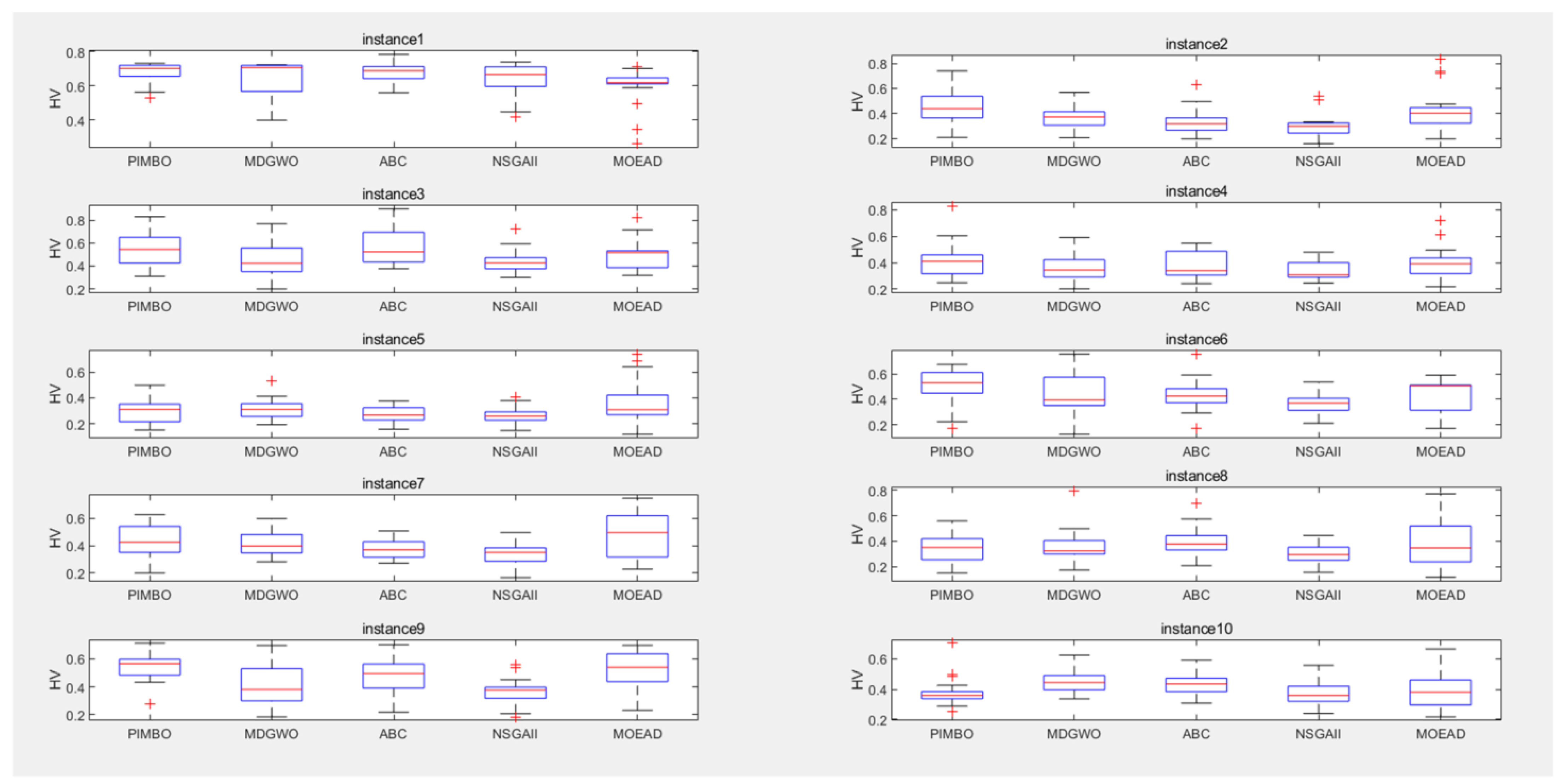
Appendix A.5. Two Boxplots

Figure A8. Boxplot of the experimental results of five algorithms via IGD metric.
Mathematics 11 01557 g0a8
Figure A9. Boxplot of the experimental results of five algorithms via hypervolume metric.
Mathematics 11 01557 g0a9

Appendix A.6. Complexity Analysis

This section analyzes the complexity of the algorithms involved in PIMBO.
(1)
Crossover operator (PPX): According to the analysis in [32], the time complexity of crossover operator is O(J), where J represents the total number of operations.
(2)
Mutation operator (PBM): According to the analysis presented in [27], the time complexity of mutation operator is O(1).
(3)
Pareto-based clustering: According to the analysis of Algorithm A1, the time complexity of Pareto-based clustering is O( Q log Q ), where Q represents the number of populations.
(4)
New individual generation: According to the analysis of Algorithm A2, the time complexity of new individual generation is O( J ), where J represents the total number of operations.

References

  1. Tian, G.; Zhou, M.; Chu, J. A Chance Constrained Programming Approach to Determine the Optimal Disassembly Sequence. IEEE Trans. Autom. Sci. Eng. 2013, 10, 1004–1013. [Google Scholar] [CrossRef]
  2. Guo, X.; Liu, S.; Zhou, M.; Tian, G. Disassembly Sequence Optimization for Large-Scale Products With Multiresource Constraints Using Scatter Search and Petri Nets. IEEE Trans. Cybern. 2015, 46, 2435–2446. [Google Scholar] [CrossRef]
  3. Güngör, A.; Gupta, S.M. Disassembly line in product recovery. Int. J. Prod. Res. 2002, 40, 2569–2589. [Google Scholar] [CrossRef]
  4. Lu, Q.; Ren, Y.; Jin, H.; Meng, L.; Li, L.; Zhang, C.; Sutherland, J.W. A hybrid metaheuristic algorithm for a profit-oriented and energy-efficient disassembly sequencing problem. Robot. Comput. Manuf. 2020, 61, 101828. [Google Scholar] [CrossRef]
  5. Li, J.; Barwood, M.; Rahimifard, S. A multi-criteria assessment of robotic disassembly to support recycling and recovery. Resour. Conserv. Recycl. 2018, 140, 158–165. [Google Scholar] [CrossRef]
  6. Çil, Z.A.; Mete, S.; Serin, F. Robotic disassembly line balancing problem: A mathematical model and ant colony optimization approach. Appl. Math. Model. 2020, 86, 335–348. [Google Scholar] [CrossRef]
  7. Wegener, K.; Chen, W.H.; Dietrich, F.; Dröder, K.; Kara, S. Robot Assisted Disassembly for the Recycling of Electric Vehicle Batteries. Procedia CIRP 2015, 29, 716–721. [Google Scholar] [CrossRef]
  8. Liu, J.; Zhou, Z.; Pham, D.T.; Xu, W.; Yan, J.; Liu, A.; Ji, C.; Liu, Q. An improved multi-objective discrete bees algorithm for robotic disassembly line balancing problem in remanufacturing. Int. J. Adv. Manuf. Technol. 2018, 97, 3937–3962. [Google Scholar] [CrossRef]
  9. Liu, J.; Zhou, Z.; Pham, D.T.; Xu, W.; Ji, C.; Liu, Q. Collaborative optimization of robotic disassembly sequence planning and robotic disassembly line balancing problem using improved discrete Bees algorithm in remanufacturing. Robot. Comput. Manuf. 2020, 61, 101829. [Google Scholar] [CrossRef]
  10. Nilakantan, J.M.; Li, Z.; Tang, Q.; Nielsen, P. Multi-objective co-operative co-evolutionary algorithm for minimizing carbon footprint and maximizing line efficiency in robotic assembly line systems. J. Clean. Prod. 2017, 156, 124–136. [Google Scholar] [CrossRef] [Green Version]
  11. Fang, Y.L.; Liu, Q.; Li, M.Q.; Laili, Y.J.; Pham, D.T. Evolutionary many-objective optimization for mixed-model disassembly line balancing with multi-robotic workstations. Eur. J. Oper. Res. 2019, 276, 160–174. [Google Scholar] [CrossRef]
  12. Pistolesi, F.; Lazzerini, B.; Mura, M.D.; Dini, G. EMOGA: A Hybrid Genetic Algorithm With Extremal Optimization Core for Multiobjective Disassembly Line Balancing. IEEE Trans. Ind. Inform. 2017, 14, 1089–1098. [Google Scholar] [CrossRef] [Green Version]
  13. Mete, S.; Çil, Z.A.; Özceylan, E.; Ağpak, K. Resource Constrained Disassembly Line Balancing Problem. IFAC-PapersOnLine 2016, 49, 921–925. [Google Scholar] [CrossRef]
  14. Wang, K.; Li, X.; Gao, L.; Garg, A. Partial disassembly line balancing for energy consumption and profit under uncertainty. Robot. Comput. Manuf. 2019, 59, 235–251. [Google Scholar] [CrossRef]
  15. Kalayci, C.B.; Polat, O.; Gupta, S.M. A variable neighbourhood search algorithm for disassembly lines. J. Manuf. Technol. Manag. 2015, 26, 182–194. [Google Scholar] [CrossRef]
  16. Homem de Mello, L.S.; Sanderson, A.C. AND/OR graph representation of assembly plan. IEEE Trans. Robot. Autom. 1990, 6, 188–199. [Google Scholar] [CrossRef] [Green Version]
  17. Guo, X.W.; Zhou, M.C.; Liu, S.X.; Qi, L. Lexicographic Multiobjective Scatter Search for the Optimization of Sequence-Dependent Selective Disassembly Subject to Multiresource Constraints. IEEE Trans. Cyber. 2019, 50, 3307–3317. [Google Scholar] [CrossRef]
  18. Bahubalendruni, M.V.A.R.; Varupala, V.P. Disassembly Sequence Planning for Safe Disposal of End-of-Life Waste Electric and Electronic Equipment. Natl. Acad. Sci. Lett. 2020, 44, 243–247. [Google Scholar] [CrossRef]
  19. Guo, X.; Zhou, M.; Abusorrah, A.; Alsokhiry, F.; Sedraoui, K. Disassembly Sequence Planning: A Survey. IEEE/CAA J. Autom. Sin. 2020, 8, 1308–1324. [Google Scholar] [CrossRef]
  20. Zhang, L.; Zhao, X.K.; Ke, Q.D.; Dong, W.F.; Zhong, Y.J. Disassembly line balancing optimization method for high efficiency and low carbon emission. Int. J. Precis. Eng. Manuf.-Green Technol. 2021, 8, 233–247. [Google Scholar] [CrossRef]
  21. Shi, Y.H. An optimization algorithm based on brainstorming process. Int. J. Swarm. Intell. Res. 2011, 2, 35–62. [Google Scholar] [CrossRef]
  22. Duan, H.; Li, S.; Shi, Y. Predator–Prey Brain Storm Optimization for DC Brushless Motor. IEEE Trans. Magn. 2013, 49, 5336–5340. [Google Scholar] [CrossRef]
  23. Duan, H.; Li, C. Quantum-Behaved Brain Storm Optimization Approach to Solving Loney’s Solenoid Problem. IEEE Trans. Magn. 2014, 51, 1–7. [Google Scholar] [CrossRef]
  24. Deb, K.; Pratap, A.; Agarwal, S.; Meyarivan, T. A fast and elitist multiobjective genetic algorithm: NSGA-II. IEEE Trans. Evol. Comput. 2002, 6, 182–197. [Google Scholar] [CrossRef] [Green Version]
  25. Bentaha, M.L.; Battaïa, O.; Dolgui, A. A sample average approximation method for disassembly line balancing problem under uncertainty. Comput. Oper. Res. 2014, 51, 111–122. [Google Scholar] [CrossRef]
  26. Gungor, A.; Gupta, S.M. A solution approach to the disassembly line balancing problem in the presence of task failures. Int. J. Prod. Res. 2001, 39, 1427–1467. [Google Scholar] [CrossRef]
  27. Zhang, Z.; Guo, X.; Zhou, M.; Liu, S.; Qi, L. Multi-objective Discrete Grey Wolf Optimizer for Solving Stochastic Multi-objective Disassembly Sequencing and Line Balancing Problem. In Proceedings of the 2020 IEEE International Conference on Systems, Man, and Cybernetics (SMC), Toronto, ON, Canada, 11–14 October 2020; pp. 682–687. [Google Scholar] [CrossRef]
  28. Xie, J.; Gao, L.; Pan, Q.-K.; Fatih, T.M. An effective multi-objective artificial bee colony algorithm for energy efficient distributed job shop scheduling. Procedia Manuf. 2019, 39, 1194–1203. [Google Scholar] [CrossRef]
  29. Zhang, Q.; Li, H. MOEA/D: A Multiobjective Evolutionary Algorithm Based on Decomposition. IEEE Trans. Evol. Comput. 2007, 11, 712–731. [Google Scholar] [CrossRef]
  30. Zhou, L.; Xiang, D.; Duan, G.H. Disassembly stability planning method in AND-OR graph model. Microcomput. Inf. 2008, 24, 1–3. [Google Scholar] [CrossRef]
  31. Fu, Y.P.; Wang, H.F.; Huang, M. Integrated scheduling for a distributed manufacturing system: A stochastic multi-objective model. Enterp. Inform. Syst. 2019, 13, 557–573. [Google Scholar] [CrossRef]
  32. Kongar, E.; Gupta, S.M. Disassembly sequencing using genetic algorithm. Int. J. Adv. Manuf. Technol. 2005, 30, 497–506. [Google Scholar] [CrossRef]
  33. Nowakowski, P. A novel, cost efficient identification method for disassembly planning of waste electrical and electronic equipment. J. Clean. Prod. 2018, 172, 2695–2707. [Google Scholar] [CrossRef]
  34. Laili, Y.J.; Li, Y.L.; Fang, Y.L.; Pham, D.T.; Zhang, L. Model review and algorithm comparison on multi-objective disassembly line balancing. J. Manuf. Syst. 2020, 56, 484–500. [Google Scholar] [CrossRef]
  35. Zitzler, E.; Thiele, L.; Laumanns, M.; Fonseca, C.M.; Da Fonseca, V.G. Performance assessment of multiobjective optimizers: An analysis and review. IEEE Trans. Evolut. Comput. 2003, 7, 117–132. [Google Scholar] [CrossRef] [Green Version]
  36. Fu, Y.; Ding, J.; Wang, H.; Wang, J. Two-objective stochastic flow-shop scheduling with deteriorating and learning effect in Industry 4.0-based manufacturing system. Appl. Soft Comput. 2018, 68, 847–855. [Google Scholar] [CrossRef]
  37. Jia, Z.X.; Duan, H.B.; Shi, Y.H. Hybrid brain storm optimisation and simulated annealing algorithm for continuous optimisation problems. Int. J. Bio-Inspir. Com. 2016, 8, 109–121. [Google Scholar] [CrossRef]
  38. Guo, X.; Wei, T.; Wang, J.; Liu, S.; Qin, S.; Qi, L. Multiobjective U-Shaped Disassembly Line Balancing Problem Considering Human Fatigue Index and an Efficient Solution. IEEE Trans. Comput. Soc. Syst. 2022, 1–13. [Google Scholar] [CrossRef]
  39. Deniz, N.; Ozcelik, F. An extended review on disassembly line balancing with bibliometric & social network and future study realization analysis. J. Clean. Prod. 2019, 225, 697–715. [Google Scholar]
  40. Guo, X.W.; Zhang, Z.W.; Qi, L.; Liu, S.X.; Tang, Y.; Zhao, Z.Y. Stochastic hybrid discrete grey wolf optimizer for multi-objective disassembly sequencing and line balancing planning in disassembling multiple products. IEEE Trans. Autom. Sci. Eng. 2022, 19, 1744–1756. [Google Scholar] [CrossRef]
  41. Ji, Y.J.; Liu, S.X.; Zhou, M.C.; Zhao, Z.Y.; Guo, X.W.; Qi, L. A machine learning and genetic algorithm-based method for predicting width deviation of hot-rolled strip in steel production systems. Inf. Sci. 2022, 589, 360–375. [Google Scholar] [CrossRef]
  42. Zhao, Z.; Liu, S.; Zhou, M.; Abusorrah, A. Dual-objective mixed integer linear program and memetic algorithm for an industrial group scheduling problem. IEEE/CAA J. Autom. Sin. 2021, 8, 1199–1209. [Google Scholar] [CrossRef]
  43. Zhao, Z.; Liu, S.; Zhou, M.; Guo, X.; Qi, L. Decomposition method for new single-machine scheduling problems from steel production systems. IEEE Trans. Autom. Sci. Eng. 2020, 17, 1376–1387. [Google Scholar] [CrossRef]
  44. Wang, W.; Tian, G.; Chen, M.; Tao, F.; Zhang, C.; Ai-Ahmari, A.; Li, Z.; Jiang, Z. Dual-objective program and improved artificial bee colony for the optimization of energy-conscious milling parameters subject to multiple constraints. J. Clean. Prod. 2019, 245, 118714. [Google Scholar] [CrossRef]
  45. Tian, Z.; Jiang, X.; Liu, W.; Li, Z. Dynamic energy-efficient scheduling of multi-variety and small batch flexible job-shop: A case study for the aerospace industry. Comput. Ind. Eng. 2023, 178, 109111. [Google Scholar] [CrossRef]
Figure 1. Part structure schematic diagram of a ballpoint pen.
Mathematics 11 01557 g001
Figure 2. Part structure schematic diagram of a lamp.
Mathematics 11 01557 g002
Figure 3. AND/OR graphs of (i) a ballpoint pen and (ii) a lamp.
Mathematics 11 01557 g003
Figure 4. An example of a robotic disassembly line layout.
Mathematics 11 01557 g004
Table 1. Products in instances.
No.12345678910
ProductsBP, WMBP, HDBP, RSHD, WMHD, RSWM, RSBP, HD, WMBP, HD, RSBP, WM, RSBP, HD, WM, RS
2595401001204512013560155
Table 2. The average running time in each instance on five algorithms.
No.Average Running Time (s)
PIMBOMDGWOMOABCNSGAIIMOEAD
12.58283.55723.54512.94222.7086
212.608523.550313.660113.181512.5823
36.730312.51899.54967.00426.7609
412.491724.732616.574215.358212.5347
520.466744.703222.123620.971120.4619
66.706812.25968.75777.25076.4053
719.154346.059223.130819.762418.5889
829.206660.166936.215730.225728.7547
911.723521.730214.772612.021911.4901
1038.817393.620951.792239.565136.6670
Table 3. The disassembly sequence and related data of instance 1 obtained by PIMBO algorithm program.
No.Disassembly Sequencef1f2f3fcrs
114,15,17---2,20,11,24---32,42,49,31978.94998.130.945963.031,2---1,3---3
214,15,17,1---21,28,38,47,27---24,12,321053.381054.990.920152.121,2---2,1,3---3,2
314,15,17,2---20,11,24,32---311069.02724.800.640428.691,2,3---1,3---3
414,15,17,1---20,24,31,32803.73654.170.900542.031,2,3---1,2,3
514,15,17,2---21,11,28,38---47,27,24,31---32,37,461524.121341.820.845260.021,2,3---1,2---1,3---2,3
614,15,17,2---20,11,24,32---6,42978.31815.960.780137.201,2---1,3---1,3
714,15,17,2---11,20,24,32---6969.73776.500.659535.461,2---1,3---1
814,15,16---2,19,11,23---30,24,32,421056.801048.140.900843.611,2,3---1,3---2,3
914,15,17,2---21,28,38,11,47---24,32,421228.711043.000.833444.211,2---1,3---3
1014,15,17,2---11,21,28,38,47---27,24,31,37---461392.761171.490.749760.561,2---1,2,3---1,3---1
Table 4. Comparison of the experimental results of the five algorithms through the C-metric.
No.C(A, B)C(B, A)t-teC(A, E)C(E, A)t-teC(A, U)C(U, A)t-teC(A, V)C(V, A)t-te
10.61290.1079+0.53920.1207+0.71890.0536+0.25550.1344+
20.69940.1245+0.80390.0514+0.91480.0113+0.14870.3698-
30.72030.0958+0.70290.0953+0.88220.0271+0.22450.3140~
40.81510.0474+0.85330.0237+0.93540.0113+0.22000.2549~
50.80550.0888+0.82840.0343+0.95430.0014+0.09920.4923-
60.56020.1932+0.64720.1226+0.87500.0230+0.31310.1614+
70.69300.1291+0.90170.0263+0.91880.0059+0.13700.4439-
80.74720.1244+0.81900.0579+0.93110.0108+0.09020.5125-
90.86080.0389+0.87740.0266+0.95800.0061+0.35390.2229+
100.81720.0524+0.90550.0263+0.96850.0043+0.11340.4556-
Table 5. Comparison of the experimental results of the five algorithms through the IGD metric.
No.PIMBOMDGWOMOABCNSGAIIMOEAD
mvt-temvt-temvt-temvt-temvt-te
10.05490.0003 0.09710.0031+0.07750.0003+0.11630.0008+0.14810.0010+
20.13600.0008 0.18650.0013+0.21040.0006+0.24780.0006+0.16930.0016+
30.10590.0005 0.17360.0030+0.16040.0008+0.20120.0009+0.14160.0011+
40.11570.0003 0.21230.0041+0.19860.0003+0.24530.0009+0.14320.0006+
50.16930.0009 0.25790.0034+0.25160.0008+0.29670.0010+0.16450.0015~
60.11150.0036 0.16730.0063+0.15580.0016+0.22960.0009+0.17330.0044+
70.15810.0005 0.21250.0031+0.24860.0008+0.28680.0006+0.16600.0013~
80.18500.0015 0.27210.0053+0.28580.0011+0.33320.0011+0.16050.0016-
90.10560.0003 0.23260.0053+0.20690.0013+0.26210.0010+0.16320.0005+
100.19590.0013 0.29280.0048+0.31940.0011+0.37970.0018+0.18720.0007~
Table 6. Comparison of the experimental results of the five algorithms through the hypervolume metric.
No.PIMBOMDGWOMOABCNSGAIIMOEAD
mvt-temvt-temvt-temvt-temvt-te
10.68030.0035 0.63990.0121~0.67880.0034~0.63840.0093~0.60000.0129+
20.45830.0159 0.37040.0088+0.33100.0105+0.29640.0089+0.42150.0289~
30.55600.0264 0.45840.0265+0.56900.0276~0.44260.0097+0.52080.0210~
40.41680.0178 0.36300.0101~0.37840.0094~0.34310.0056+0.39880.0136~
50.29800.0078 0.31150.0064~0.27150.0040~0.26250.0040~0.35870.0282~
60.51020.0202 0.44870.0258~0.43210.0142+0.37020.0072+0.42990.0158+
70.42820.0155 0.41180.0076~0.37610.0053~0.34370.0063+0.46810.0261~
80.34140.0146 0.36480.0172~0.39490.0122~0.29700.0060~0.38410.0329~
90.54340.0090 0.40900.0213+0.48150.0139+0.36860.0085+0.50950.0209~
100.38030.0091 0.45040.0053-0.43830.0055-0.37450.0067~0.38550.0125~
Disclaimer/Publisher’s Note: The statements, opinions and data contained in all publications are solely those of the individual author(s) and contributor(s) and not of MDPI and/or the editor(s). MDPI and/or the editor(s) disclaim responsibility for any injury to people or property resulting from any ideas, methods, instructions or products referred to in the content.

