Periodically Intermittent Control of Memristor-Based Hyper-Chaotic Bao-like System

Abstract

In this paper, based on a three-dimensional Bao system, a memristor-based hyper-chaotic Bao-like system is successfully constructed, and a simulated equivalent circuit is designed, which is used to verify the chaotic behaviors of the system. Meanwhile, a control method called periodically intermittent control with variable control width is proposed. The control width sequence in the proposed method is not only variable, but also monotonically decreasing, and the method can effectively stabilize most existing nonlinear systems. Moreover, the memristor-based hyper-chaotic Bao-like system is controlled by combining the proposed method with the Lyapunov stability principle. Finally, we should that the proposed method can effectively control and stabilize not only the proposed hyper-chaotic system, but also the Chua’s oscillator.

1. Introduction

For decades, the mystery of chaotic phenomena has been explored. Lorenz established the Lorenz system [1] in 1963 when he studied the phenomenon of atmospheric turbulence. In 2009, Bao et al. [2] made a mirror transformation of the first two equations of state in the Lü system equation [3], and the nonlinearity term in the third state equation is modified by $x^2$, a three-dimensional Bao system with more complex chaotic behaviors is obtained. Compared with the three-dimensional chaotic system, the hyper-chaotic system has more complex dynamics, which can be obtained by adding a state feedback controller to the three-dimensional chaotic system [4,5]. In [4], two linear terms are added as a linear state feedback controller to a continuous chaotic system to obtain a hyper-chaotic system, and the basic dynamical behaviors of the hyper-chaotic system are analyzed using numerical simulations. In [5], two nonlinear terms are added as a nonlinear state feedback controller to the Lorenz system to construct a hyper-chaotic system, and the simulation circuit is designed for the hyper-chaotic system.

The memristor was put forward by Chua [6] in 1971, which was physically realized by Strukov et al. [7] in 2008. Meanwhile, memristor has also been utilized in the fields of communication engineering, neural networking, and bioengineering, and have yielded many pleasant results [8,9,10,11]. In recent years, researches on memristors have been of great interests, and many results [12,13] have emerged. In [12], a memristor model is constructed, and the chaotic characteristics of the memristor are measured using circuit simulation. In [13], a novel discrimination method for memristor is proposed, and a new memristor model is constructed. The necessary condition for the construction of chaotic systems is nonlinearity, and the memristor has this feature, which can be utilized to design a new chaotic system. There are many research results about the memristor-based chaotic system [14,15,16]. In [14], oscillators with many rich oscillation characteristics and nonlinear dynamical behaviors are obtained by substituting Chua’s diode for a memristor. In [15], a new memristor-based hyper-chaotic system is obtained by combining a Hewlett Packard (HP) memristor with a four-dimensional continuous system, and an equivalent analog circuit is designed to verify its chaotic behaviors. In [16], a memristor-based chaotic system is obtained by substituting a memristor for Chua’s diode, and its basic dynamical properties are analyzed using numerical simulations. Furthermore, its chaotic behaviors are verified with circuit experimental results. On the basis of [2], a smooth cubic nonlinear flux-controlled memristor and a linear term as a nonlinear state feedback controller are added to the equations of the three-dimensional Bao system so that the memristor-based hyper-chaotic Bao-like system in this paper is obtained. For the hyper-chaotic system, complex chaotic behaviors are relatively easy to generate due to the existence of a memristor.

Generally speaking, in order to stabilize a class of nonlinear systems, people will add a feedback mechanism. Recently, some useful and effective control strategies, such as impulsive control [17,18,19,20,21,22] and intermittent control [23,24,25,26] have been favored by many scholars. In [17], Xie et al. analyzed the stability of the Chen hyper-chaotic system using the three-stage-impulse control method. In [18], Yang et al. designed an impulsive controller with a time delay to achieve exponential synchronization between the two systems, and the results of this theory were also applied to secure communication. In [19], Rao et al. constructed an epidemic model with delayed impulse, and also gave a new synchronization method. In [20], Wu et al. utilized a set of adaptive uncertain control matrices for impulsive control of nonlinear systems, and numerical simulation examples were used to demonstrate the superiority of the method. In [21], Chen et al. constructed a system and analyzed the stability of the system by using some inequality principles. In addition, numerical simulation examples were used to demonstrate the validity of the theory. Ref. [23] studied the exponential stability of a class of nonlinear systems using periodically intermittent control. Ref. [25] studied the dissipative performance of distributed parameter systems by using a fuzzy aperiodic intermittent sampling data control method, and in order to save control cost, the optimal control gain was given. Also, numerical simulation examples were used to prove the feasibility of the method. Ref. [26] analyzed the stability of a class of systems with random factors and delays by using intermittent control, and by using numerical simulation, the effectiveness of the method was proven. As a result of the convenience and efficiency of intermittent control, it has been applied to many fields such as medicine, communication engineering, transportation, and so on.

In recent years, intermittent control has been used to study the stability [27,28,29,30], and synchronization of chaotic systems [31,32,33,34,35]. For the former, Ref. [27] studied the stabilization of delayed dynamical systems by using the dynamic event-triggered intermittent control. Ref. [28] analyzed the stabilization of complex-valued stochastic networks by using periodic self-triggered intermittent control. For the latter, in [32], the finite-time synchronization of uncertain nonlinear systems containing perturbations was realized by using aperiodic intermittent control. In [35], the prefixed-time synchronization of a class of dynamic networks with delay was achieved by using local intermittent sampling control, and a numerical example was used to verify the feasibility of the method.

However, in practical problems, the control width sequence of intermittent control may change. Whether the former or the latter, the control width sequence is fixed, which may lead to some limitations in real life. Therefore, in order to remove this limitation, on the basis of [23], a periodically intermittent control method with variable control width is proposed in this paper. In this new method, the control width sequence is not only variable, but also monotonically decreasing. Therefore, compared with the traditional method, this new method may have wider practicability. In addition, the proposed method is used to control the proposed hyper-chaotic system and the Chua’s oscillator in this paper.

In summary, the outstanding contributions of this paper are listed below:

(i)

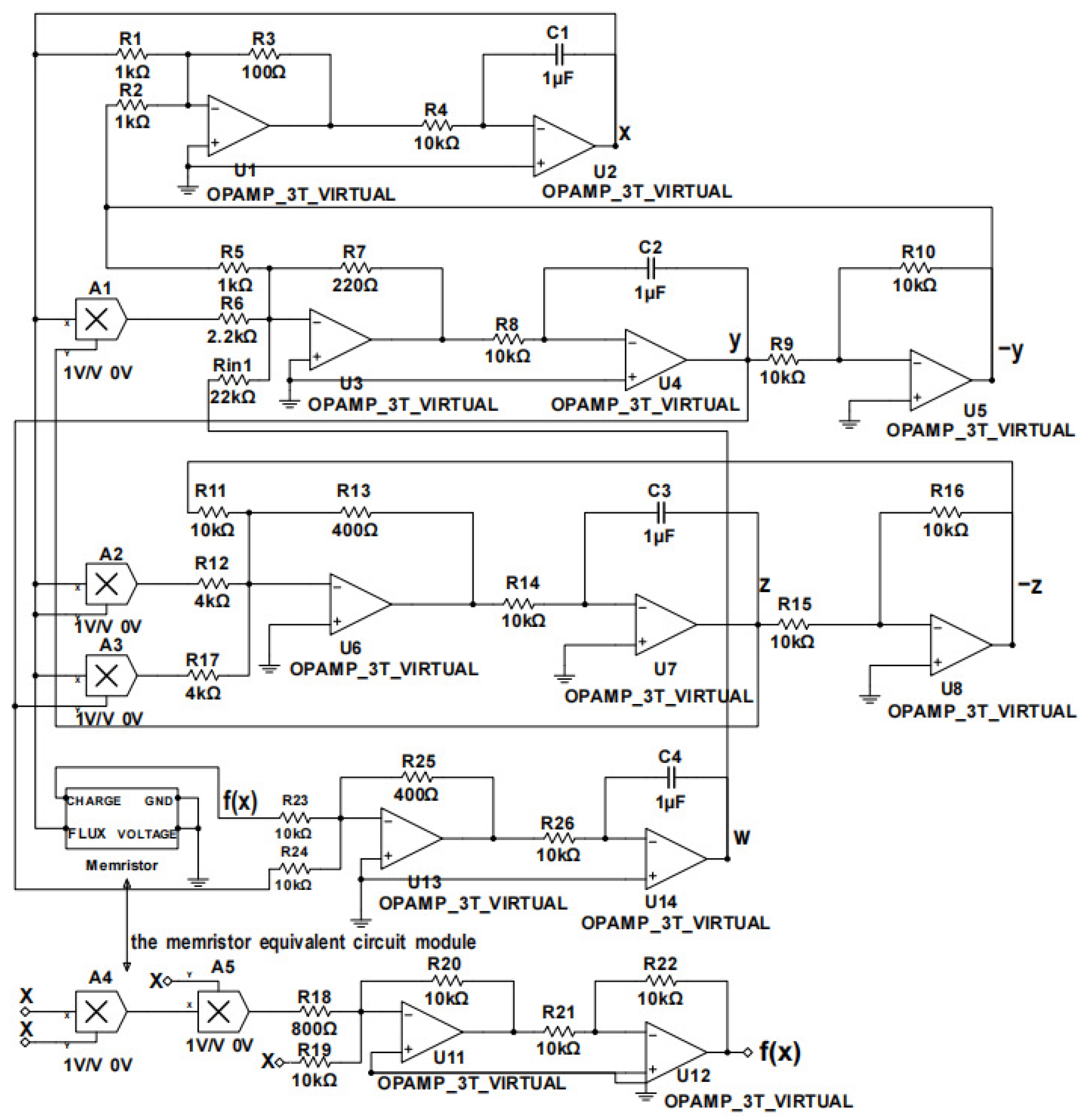
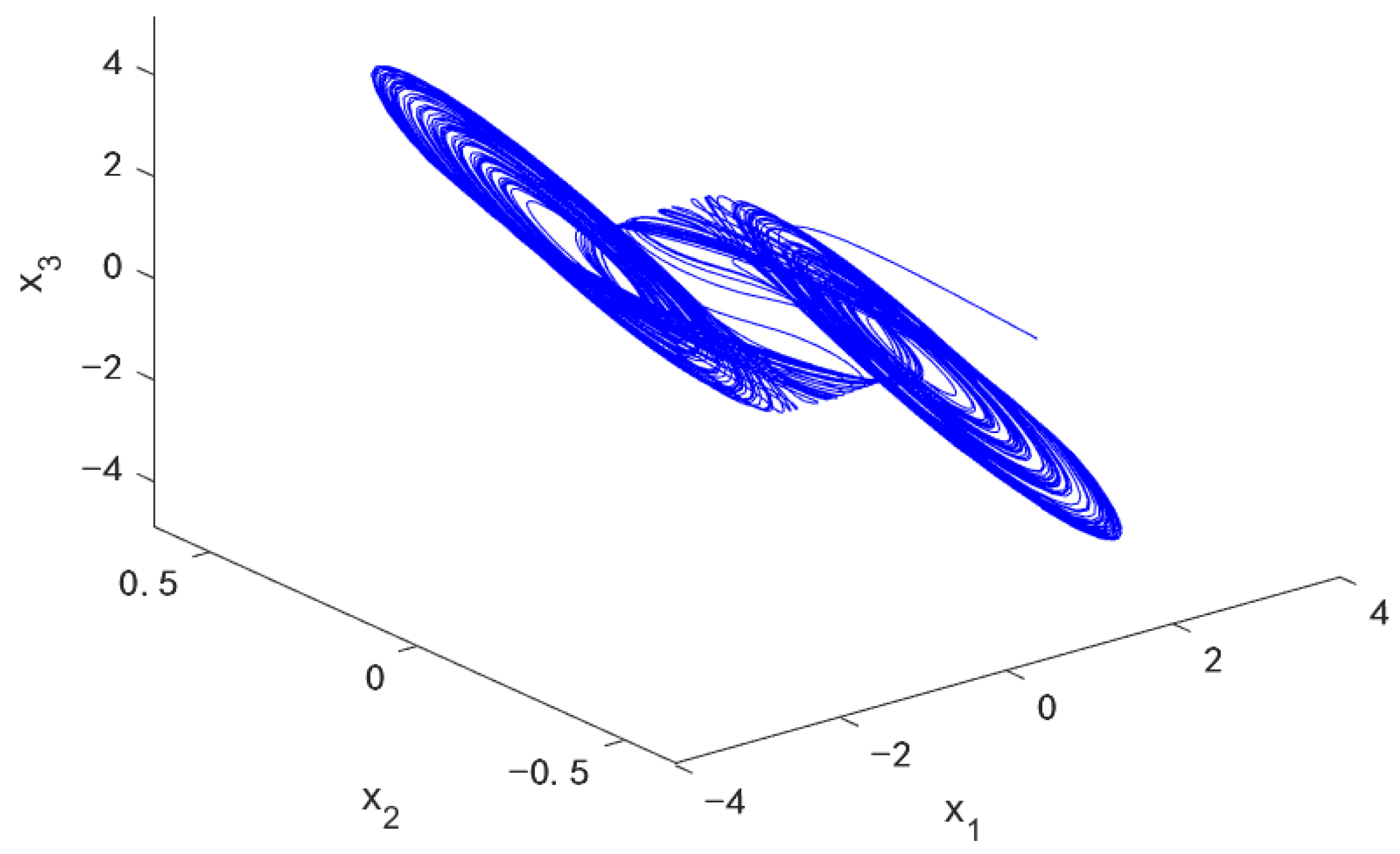
A memristor-based hyper-chaotic Bao-like system is constructed, and its chaotic behavior is verified by designing an analog circuit;

(ii)

A novel control method called periodically intermittent control with variable control width is proposed, and the proposed hyper-chaotic system is controlled by this method.

This paragraph contains the outline of the remaining part of this paper. In Section 2, the memristor-based hyper-chaotic Bao-like system is constructed, and its mathematical model and the circuit implementation are given; in Section 3, the general nonlinear system, the design of the controller and some lemmas and mathematical knowledge to be used in this paper are introduced; in Section 4, a method called periodically intermittent control with variable control width is proposed, and some conditions about the exponential stability of a classical nonlinear system are obtained; in Section 5, in order to verify the feasibility of the method, the proposed method is used to stabilize the hyper-chaotic system and the Chua’s oscillator, and their simulation results are also given. Finally, Section 6 summarizes this paper.

Notation 1.

The maximum eigenvalue, the minimum eigenvalue, and the transpose of square matrix Q are represented by ${\lambda }_H\left(Q\right),{\lambda }_h\left(Q\right),$ and $Q^T$, respectively. The Euclidean norm of the vector x is represented by $∥x∥$, I denotes the identity matrix.

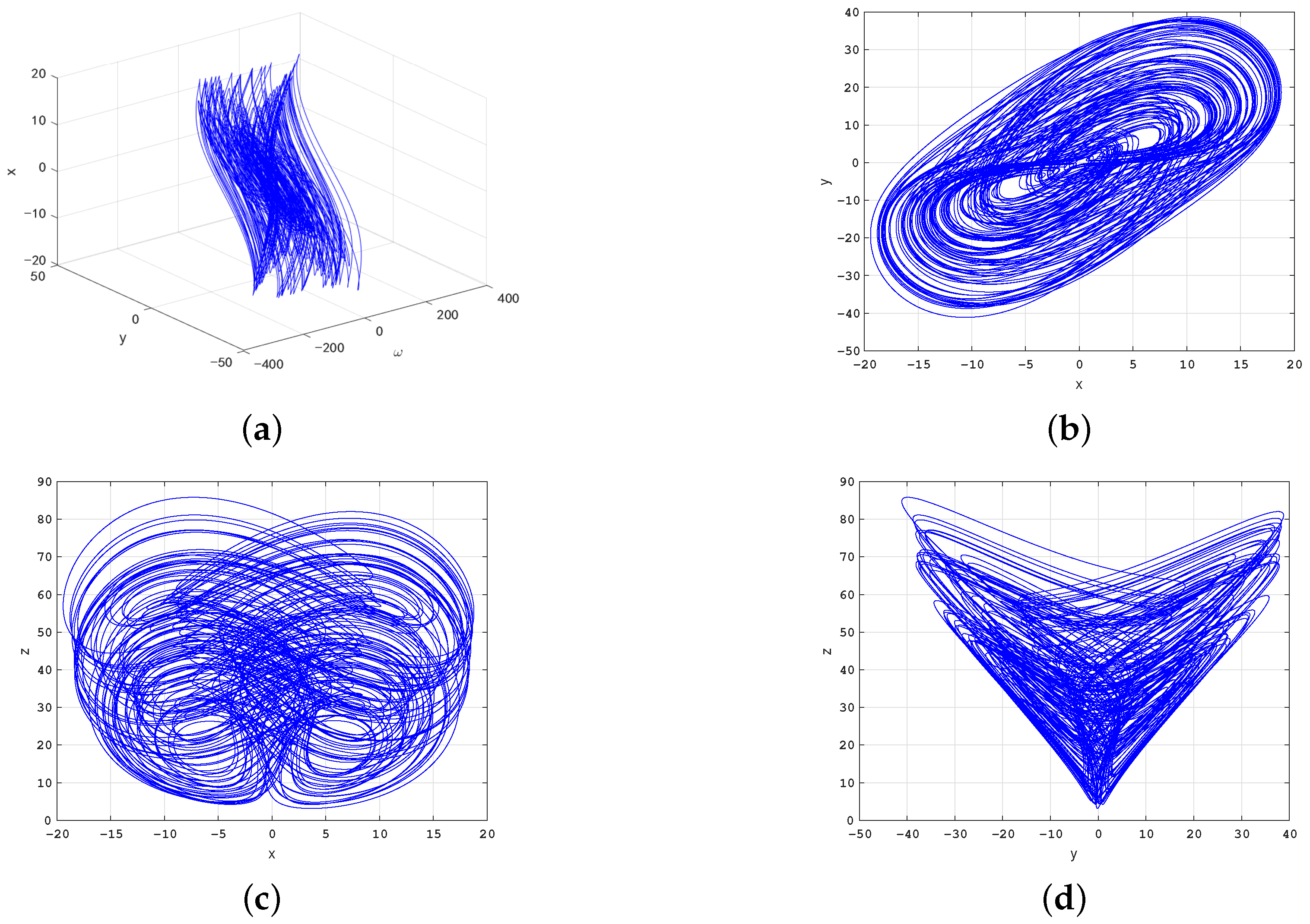
2. Construction of the New Hyper-Chaotic System

The mathematical model of the Bao system [2] can be described by the following set of differential equations

$$\left\{\begin{array}{c}\dot{x}=a\left(x-y\right),\hfill \\ \dot{y}=xz-cy,\hfill \\ \dot{z}=x^2-bz,\hfill \end{array}\right.$$

(1)

where x, y, and z are the state vectors of the system. Further, a, b, and c are positive real parameters.

Figure 1 shows the circuit configuration and structure of the Bao chaotic system, which is implemented in an analog circuit using mainly operational amplifiers, multipliers, resistors and capacitors.

According to Kirchhoff’s Current Law (KCL) and Kirchhoff’s Voltage Law (KVL) [36], the circuit can be described by the following differential equations:

$$\left\{\begin{array}{c}{\displaystyle \dot{x}=\frac{x{R}_3}{R_1{R}_4{C}_1}-\frac{y{R}_3}{R_2{R}_4{C}_1},}\hfill \\ \\ {\displaystyle \dot{y}=\frac{xz{R}_7{R}_{10}}{R_6{R}_8{R}_9{C}_2}-\frac{y{R}_7{R}_{10}}{R_5{R}_8{R}_9{C}_2},}\hfill \\ \\ {\displaystyle \dot{z}=\frac{x^2{R}_{13}{R}_{16}}{R_{12}{R}_{14}{R}_{15}{C}_3}-\frac{z{R}_{13}{R}_{16}}{R_{11}{R}_{14}{R}_{15}{C}_3}.}\hfill \end{array}\right.$$

(2)

By comparing (2) with the parameters in system (1), we can obtain the values of each component in Figure 1.

It is well known that the necessary condition for the creation of chaotic systems is nonlinearity, and the memristor has this feature. Therefore, in order for the system to generate more complex chaotic behaviors, a flux-controlled memristor model [37], a linear feedback term, and a nonlinear feedback term are added to the Bao chaotic system. The mathematical model of the flux-controlled memristor can be described by a smooth monotonically rising cubic nonlinear curve equation

$$q\left(\phi \right)=\alpha \phi +\beta {\phi }^3,$$

(3)

where $\alpha$ and $\beta$ are positive constants. Furthermore, q and $\phi$ represent the charge and flux of the memristor, respectively.

For convenience, let $x=\phi ,$$f=q$, and (3) is rewritten as follows:

$$f\left(x\right)=\alpha x+\beta x^3.$$

(4)

On the basis of (4), a new variable $\omega$ as the excitation is introduced into the Bao chaotic system, so a memristor-based hyper-chaotic Bao-like system is obtained, and the mathematical model of the hyper-chaotic system can be described by the following set of differential equations

$$\left\{\begin{array}{c}\dot{x}=a\left(x-y\right),\hfill \\ \dot{y}=xz-cy+w,\hfill \\ \dot{z}=x^2-bz+xy,\hfill \\ \dot{\omega }=dy+f\left(x\right),\hfill \end{array}\right.$$

(5)

in which x, y, z, and $\omega$ are the state vectors of the system. Additionally, a, b, c, and d are positive real parameters. $f\left(x\right)$ is a nonlinear function that represents the relationship between the flux and the charge of the memristor.

After the transformation of system (5) with $\left(x,y,z,\omega \right)\to \left(-x,-y,-z,-\omega \right)$, the equation of the system remains unchanged, so the system is symmetric about the z axis. In addition, the dissipation of system (5) can be calculated with the following equation

$$\nabla V_M=\frac{\partial \dot{x}}{\partial x}+\frac{\partial \dot{y}}{\partial y}+\frac{\partial \dot{z}}{\partial z}+\frac{\partial \dot{\omega }}{\partial \omega }=a-b-c<0,$$

(6)

in which $\nabla V_M$ is used to denote the dissipativity.

Therefore, from the above results, when the values of system parameters a, b, and c satisfy (6), the dissipation of system (5) can be guaranteed. In other words, the trajectory of system (5) will eventually converge to zero.

It is extremely important to obtain and analyze the equilibrium point of a chaotic system, which can be used to study the stability of the equilibrium point of the system. Thus, the Jacobi matrix $J_v^{*}$ at the equilibrium point $S_v^{*}=\left(x_v^{*},y_v^{*},z_v^{*},{\omega }_v^{*}\right)$ of system (5) is defined as follows:

$$J_v^{*}=\left[\begin{array}{cccc}a& -a& 0& 0\\ z_v^{*}& -c& 0& 1\\ x_v^{*}+y_v^{*}& x_v^{*}& -b& 0\\ \alpha +3\beta {\left(x_v^{*}\right)}^2& d& 0& 0\end{array}\right].$$

(7)

To obtain the values of the equilibrium point of the system, let $\dot{x}=\dot{y}=\dot{z}=\dot{\omega }=0$. Obviously, the equilibrium point $S_v^{*}=\left(0,0,0,0\right)$ is the only equilibrium point of the system. Moreover, the following characteristic equation can be obtained by (7):

$$\left(b+\lambda \right)\left({\lambda }^3+\left(c-a\right){\lambda }^3+\left(ac+d\right)\lambda -\left(d+\alpha \right)a\right)=0.$$

(8)

Therefore, the equilibrium point $S_v^{*}=\left(0,0,0,0\right)$ is unstable using the Routh–Hurwitz criterion.

In order to make system (5) exhibit chaotic dynamics behavior, let the parameters $a=10$, $b=4$, $c=22$, $d=4$, $\alpha =4$, and $\beta =0.5$. The chaotic attractor phase diagram of the memristor-based hyper-chaotic Bao-like system with the initial condition $\mathbf{x}\left(0\right)={\left[x\left(0\right),y\left(0\right),z\left(0\right),\omega \left(0\right)\right]}^T={\left[10,10,10,10\right]}^T$ is shown in Figure 2, where Figure 2a, Figure 2b, Figure 2c, and Figure 2d, represent attractor phase diagrams of the x-y-$\omega$ plane, x-y plane, x-z plane, and y-z plane, respectively.

The concept of the Lyapunov exponent was first introduced in [38] and can be used to characterize the motion of the system. When a system contains no less than one positive Lyapunov exponent, it can be determined whether it is chaotic [39]. The Lyapunov exponents of system (5) can be calculated by using the Wolf method in [38], and Figure 3 shows the Lyapunov exponential spectrum of the hyper-chaotic system. To show more clearly, combined with the data analysis in

Table 1. Lyapunov exponents.

Time	${\mathit{LE}}_1$	${\mathit{LE}}_2$	${\mathit{LE}}_3$	${\mathit{LE}}_4$
$t=0.3$	8.6789	2.9300	−3.8563	−23.7506
$t=0.6$	7.1126	−1.2834	−0.0935	−21.7304
⋮	⋮	⋮	⋮	⋮
$t=59.7$	0.4827	0.1783	−0.0079	−16.3812
$t=60.0$	0.5369	0.1863	−0.0077	−16.4081

, the Lyapunov exponents that $L{E}_1=0.5369$, $L{E}_2=0.1863$, $L{E}_3=-0.0077\approx 0$, and $L{E}_4=-16.4081$ can be obtained respectively. The Kaplan–Yorke dimension [40] of the hyper-chaotic system is defined as:

$$D_L=j+\frac{{\displaystyle \sum _{i=1}^{i=j}}L{E}_i}{\left||L{E}_{j+1}|\right|}=3+\frac{0.5369+0.1863-0.0077}{\left||-16.4081|\right|}=3.07,$$

(9)

where j represents the largest integer.

In order to verify the chaotic behavior of system (5), the modular circuit of the hyper-chaotic system is designed, as shown in Figure 4. Additionally, the modular circuit of the cubic nonlinear flux-controlled memristor is composed of two operational amplifiers, two multipliers, and five resistors.

Similarly, according to KCL and KVL, the circuit can be described by the following differential equations

$$\left\{\begin{array}{c}{\displaystyle \dot{x}=\frac{x{R}_3}{R_1{R}_4{C}_1}-\frac{y{R}_3}{R_2{R}_4{C}_1},}\hfill \\ \\ {\displaystyle \dot{y}=\frac{xz{R}_7{R}_{10}}{R_6{R}_8{R}_9{C}_2}-\frac{y{R}_7{R}_{10}}{R_5{R}_8{R}_9{C}_2}+\frac{\omega R_7{R}_{10}}{R_{in}{R}_8{R}_9{C}_2},}\hfill \\ \\ {\displaystyle \dot{z}=\frac{x^2{R}_{13}{R}_{16}}{R_{12}{R}_{14}{R}_{15}{C}_3}-\frac{z{R}_{13}{R}_{16}}{R_{11}{R}_{14}{R}_{15}{C}_3}+\frac{xy{R}_{13}{R}_{16}}{R_{17}{R}_{14}{R}_{15}{C}_3},}\hfill \\ \\ {\displaystyle \dot{\omega }=\frac{x^3{R}_{20}{R}_{22}{R}_{25}}{R_{19}{R}_{21}{R}_{23}{R}_{26}{C}_4}+\frac{x{R}_{20}{R}_{22}{R}_{25}}{R_{18}{R}_{21}{R}_{23}{R}_{26}{C}_4}+\frac{y{R}_{25}}{R_{24}{R}_{26}{C}_4}.}\hfill \end{array}\right.$$

(10)

By comparing (10) with the parameters in system (5), we can obtain the values of each component in Figure 4. Figure 5 shows the phase diagram of the chaotic attractor observed on the oscilloscope. By comparison, it is basically consistent with the simulation results in Figure 2.

Remark 1.

In the actual circuit, the absolute value of the supply voltage of the operational amplifier does not exceed $15v$, and the absolute value of the supply voltage of the analog multiplier does not exceed $10v$. Therefore, in this circuit, the supply voltage of the operational amplifier, and the analog multiplier is set to $\pm 15v$ and $\pm 9v$, respectively. From the chaotic attractor phase diagram in Figure 2, the dynamic range of the chaotic attractor of system (5) is within $\pm 100$. Thus, without changing the performance of the system, the size of all four state variables of the system are uniformly compressed to ${\displaystyle \frac{1}{10}}$ of the original size.

3. Introduction of the Periodically Intermittent Control

The following is a classical nonlinear system:

$$\left\{\begin{array}{c}\dot{x}\left(t\right)=Bx\left(t\right)+Cg\left(x\left(t\right)\right)+\delta \left(t\right),\hfill \\ x\left(t_0\right)=x_{0,}\hfill \end{array}\right.$$

(11)

where $x\in R^n$ is a state vector, $B,C\in R^{n\times n}$ are constant matrices, and $g:R^n\to R^n$ is a continuous nonlinear function that satisfies $g\left(0\right)=0$. Suppose that there is a diagonal matrix $L=\mathrm{diag}\left(b_1,b_2,\cdots ,b_n\right)\ge 0$ such that ${∥g\left(x\right)∥}^2\le x^{T}Lx$ for arbitrary $x\in R^n$. $\delta \left(t\right)$ is the external input of system (11) which can be described as

$$\delta \left(t\right)=\left\{\begin{array}{cc}Kx\left(t\right),\hfill & \varrho T\le t<\varrho T+{\tau }_{\varrho },\hfill \\ 0,\hfill & \varrho T+{\tau }_{\varrho }\le t<\left(\varrho +1\right)T.\hfill \end{array}\right.$$

(12)

So, system (11) can be written as

$$\left\{\begin{array}{cc}\dot{x}\left(t\right)=Bx\left(t\right)+Cg\left(x\left(t\right)\right)+Kx\left(t\right),\hfill & \varrho T\le t<\varrho T+{\tau }_k,\hfill \\ \dot{x}\left(t\right)=Bx\left(t\right)+Cg\left(x\left(t\right)\right),\hfill & \varrho T+{\tau }_{\varrho }\le t<\left(\varrho +1\right)T,\hfill \\ x\left(t_0\right)=x_0,\hfill & \end{array}\right.$$

(13)

in which $K\in R^{n\times n}$ is a constant matrix that represents the control intensity. $\left\{{\tau }_{\varrho }\right\}$ represents the control width sequence, satisfying $0<{\tau }_{\varrho }\le T,\varrho =0,1,2,\cdots$, and $T>0$ denotes the period of control. In addition, ${\tau }_{\varrho }$ also satisfies the following equation

$${\tau }_{\varrho }={\tau }_0-\varrho d,$$

(14)

in which ${\tau }_0=T$, and $d\ge 0$ represent the variance.

The method in (13) is called periodically intermittent control method.

Remark 2.

Let ${\tau }_0=\zeta$, and $d=0$, in which $\zeta \in \left(0,T\right)$. Then, system (13) becomes the case in [23].

In addition, in order to make system (13) stable, the following two lemmas need to be used.

Lemma 1

([41]). For any three real matrices ${\varphi }_1,{\varphi }_{2,}{\varphi }_3\in R^{n\times m}$, $0<{\varphi }_3={\varphi }_3^T$, and a scalar $\mu \ge 0$, we have the following inequality:

$${\varphi }_1^T{\varphi }_2+{\varphi }_2^T{\varphi }_1\le \mu {\varphi }_1^T{\varphi }_3{\varphi }_1+{\mu }^{-1}{\varphi }_2^T{\varphi }_3^{-1}{\varphi }_2.$$

(15)

Lemma 2

([42]). Let ${\rm Y}\left(x\right)={{\rm Y}}^T\left(x\right),\Psi \left(x\right)={\Psi }^T\left(x\right)$, and

$$\left[\begin{array}{cc}{\rm Y}\left(x\right)& \Phi \left(x\right)\\ {\Phi }^T\left(x\right)& \Psi \left(x\right)\end{array}\right]>0,$$

(16)

Therefore, the above linear matrix inequality (LMI) can be rewritten as the following

$$\Psi \left(x\right)>0,{\rm Y}\left(x\right)-\Phi \left(x\right){\Psi }^{-1}\left(x\right){\Phi }^T\left(x\right)>0.$$

4. Main Results

This section analyzes the exponential stability of system (13) by constructing a Lyapunov-like method, and obtains the conditions for judging exponential stability and a corollary about exponential stability.

Theorem 1.

Suppose there exists a symmetric and positive definite matrix $Q>0$, four positive scalar constants ${\mu }_1>0$, ${\mu }_2>0$, $p_1>0$, and $p_2>0$ satisfying the following conditions:

(i) 

$QB+B^{T}Q+QK+K^{T}Q+{\mu }_{1}QC{C}^{T}Q+{\mu }_1^{-1}L+p_{1}Q\le 0$;

(ii) 

$QB+B^{T}Q+{\mu }_{2}QC{C}^{T}Q+{\mu }_2^{-1}L-p_{2}Q\le 0$;

(iii) 

$p_1\ge p_2$.

Then the origin of system (13) is determined to be exponentially stable, and moreover

$$\parallel x\left(t\right)\parallel \le \sqrt{\frac{{\lambda }_H\left(Q\right)}{{\lambda }_h\left(Q\right)}}\parallel x_0\parallel exp\left\{-p_2\frac{t}{2T}{\tau }_l+\frac{p_1}{2}{\tau }_l\right\},\forall t>0.$$

(17)

Proof. 

The following Lyapunov function needs to be constructed

$$V\left(x\left(t\right)\right)=x^T\left(t\right)Qx\left(t\right),$$

(18)

which implies that

$${\lambda }_h\left(Q\right)\parallel x\left(t\right)\parallel \le V\left(x\left(t\right)\right)\le {\lambda }_H\left(Q\right)\parallel x\left(t\right)\parallel .$$

(19)

When $\varrho T\le t<\varrho T+{\tau }_{\varrho }$, the state of system (13) can be calculated and estimated by using Lemma 1 and (18) as follows:

$$\begin{array}{cc}\hfill \dot{V}\left(x\right)& =2x^{T}Q\dot{x}\hfill \\ \hfill & =2x^{T}Q\left(Bx+Cg\left(x\right)+Kx\right)\hfill \\ \hfill & =2x^{T}QBx+2x^{T}QCg\left(x\right)+2x^{T}QKx\hfill \\ \hfill & =x^T\left(QB+B^{T}Q+QK+K^{T}Q\right)x+2x^{T}QCg\left(x\right)\hfill \\ \hfill & \le x^T\left(QB+B^{T}Q+QK+K^{T}Q\right)x+{\mu }_1{x}^{T}QC{C}^{T}Qx+{\mu }_1^{-1}{x}^{T}Lx\hfill \\ \hfill & =x^T\left(QB+B^{T}Q+QK+K^{T}Q+{\mu }_{1}QC{C}^{T}Q\right.\left.+{\mu }_1^{-1}L+p_{1}Q\right)x-p_{1}V\left(x\right)\hfill \\ \hfill & \le -p_{1}V\left(x\right),\hfill \end{array}$$

where $QB+B^{T}Q+QK+K^{T}Q+{\mu }_{1}QC{C}^{T}Q+{\mu }_1^{-1}L+p_{1}Q\le 0$. Therefore, it can be obtained that

$$V\left(x\left(t\right)\right)\le V\left(x\left(\varrho T\right)\right)exp\left(-p_1\left(t-\varrho T\right)\right),$$

(20)

where $\varrho T\le t<\varrho T+{\tau }_{\varrho }$.

Similarly, when $\varrho T+{\tau }_{\varrho }\le t<\left(\varrho +1\right)T$, then it can be obtained that

$$\begin{array}{cc}\hfill \dot{V}\left(x\right)& =2x^{T}Q\dot{x}\hfill \\ \hfill & =2x^{T}Q\left(Bx+Cg\left(x\right)\right)\hfill \\ \hfill & =2x^{T}QBx+2x^{T}QCg\left(x\right)\hfill \\ \hfill & \le x^T\left(QB+B^{T}Q\right)x+{\mu }_2{x}^{T}QC{C}^{T}Qx+{\mu }_2^{-1}{x}^{T}Lx\hfill \\ \hfill & =x^T\left(QB+B^{T}Q+{\mu }_{2}QC{C}^{T}Q+{\mu }_2^{-1}L-p_{2}Q\right)x+p_{2}V\left(x\right)\hfill \\ \hfill & \le p_{2}V\left(x\right),\hfill \end{array}$$

where $QB+B^{T}Q+{\mu }_{2}QC{C}^{T}Q+{\mu }_2^{-1}L-p_{2}Q\le 0$. Therefore, it can be obtained that

$$V\left(x\left(t\right)\right)\le V\left(x\left(\varrho T+{\tau }_{\varrho }\right)\right)exp\left(p_2\left(t-\varrho T-{\tau }_{\varrho }\right)\right),$$

(21)

where $\varrho T+{\tau }_{\varrho }\le t<(\varrho +1)T$.

Then, from (20) and (21), the following results can be obtained by using mathematical induction:

Case 1: $\varrho =0$

Subcase 1: When $0\le t<{\tau }_0$, it can be obtained that

$$\begin{array}{cc}\hfill V\left(x\left(t\right)\right)& \le V\left(x_0\right)exp\left(-p_{1}t\right),\hfill \end{array}$$

therefore,

$$\begin{array}{cc}\hfill V\left(x\left({\tau }_0\right)\right)& \le V\left(x_0\right)exp\left(-p_1{\tau }_0\right).\hfill \end{array}$$

Subcase 2: When ${\tau }_0\le t<T$, then

$$\begin{array}{cc}\hfill V\left(x\left(t\right)\right)& \le V\left(x\left({\tau }_0\right)\right)exp\left\{p_2\left(t-{\tau }_0\right)\right\}\hfill \\ \hfill & \le V\left(x_0\right)exp\left\{-p_1{\tau }_0+p_2\left(t-{\tau }_0\right)\right\},\hfill \end{array}$$

therefore,

$$\begin{array}{c}\hfill V\left(x\left(T\right)\right)\le V\left(x_0\right)exp\left\{-p_1{\tau }_0+p_2\left(T-{\tau }_0\right)\right\}.\end{array}$$

Case 2: $\varrho =1$

Subcase 1: When $T\le t<T+{\tau }_1$, it can be obtained that

$$\begin{array}{cc}\hfill V\left(x\left(t\right)\right)& \le V\left(x\left(T\right)\right)exp\left\{-p_1\left(t-T\right)\right\}\hfill \\ \hfill & \le V\left(x_0\right)exp\left\{-p_1\left(t-T+{\tau }_0\right)+p_2\left(T-{\tau }_0\right)\right\},\hfill \end{array}$$

therefore,

$$\begin{array}{c}\hfill V\left(x\left(T+{\tau }_1\right)\right)\le V\left(x_0\right)exp\left\{-p_1\sum _{i=0}^1{\tau }_i+p_2\left(T-{\tau }_0\right)\right\}.\end{array}$$

Subcase 2: When $T+{\tau }_1\le t<2T$, then

$$\begin{array}{cc}\hfill V\left(x\left(t\right)\right)& \le V\left(x\left(T+{\tau }_1\right)\right)exp\left\{p_2\left(t-T-{\tau }_1\right)\right\}\hfill \\ \hfill & \le V\left(x_0\right)exp\left\{-p_1\left({\tau }_0+{\tau }_1\right)+p_2\left(t-{\tau }_0-{\tau }_1\right)\right\},\hfill \end{array}$$

therefore,

$$\begin{array}{c}\hfill V\left(x\left(2T\right)\right)\le V\left(x_0\right)exp\left\{-p_1\sum _{i=0}^1{\tau }_i+p_2\left(2T-\sum _{i=0}^1{\tau }_i\right)\right\}.\end{array}$$

Similarly, the following results can be obtained by using mathematical induction:

Case $l+1$: $\varrho =l$

Subcase 1: When $lT\le t<lT+{\tau }_l$, it can be obtained that

$$\begin{array}{cc}\hfill V\left(x\left(t\right)\right)& \le V\left(x\left(lT\right)\right)exp\left\{-p_1\left(t-lT\right)\right\}\hfill \\ \hfill & \le V\left(x_0\right)exp\left\{-p_1\left(t-lT+\sum _{i=0}^{l-1}{\tau }_i\right)+p_2\left(lT-\sum _{i=0}^{l-1}{\tau }_i\right)\right\}.\hfill \end{array}$$

therefore,

$$\begin{array}{cc}\hfill V\left(x\left(lT+{\tau }_l\right)\right)& \le V\left(x_0\right)exp\left\{-p_1\left(\sum _{i=0}^l{\tau }_i\right)+p_2\left(lT-\sum _{i=0}^{l-1}{\tau }_i\right)\right\}.\hfill \end{array}$$

Subcase 2: When $lT+{\tau }_l\le t<(l+1)T$, it can be obtained that

$$\begin{array}{cc}\hfill V\left(x\left(t\right)\right)& \le V\left(x\left(lT+{\tau }_l\right)\right)exp\left\{p_2\left(t-lT-{\tau }_l\right)\right\}\hfill \\ \hfill & \le V\left(x_0\right)exp\left\{-p_1\left(\sum _{i=0}^l{\tau }_i\right)+p_2\left(t-\sum _{i=0}^l{\tau }_i\right)\right\},\hfill \end{array}$$

therefore,

$$\begin{array}{cc}\hfill V\left(x\left(\left(l+1\right)T\right)\right)& \le V\left(x_0\right)exp\left\{-p_1\left(\sum _{i=0}^l{\tau }_i\right)+p_2\left(\left(l+1\right)T-\sum _{i=0}^l{\tau }_i\right)\right\}.\hfill \end{array}$$

In addition, when $lT\le t<lT+{\tau }_l$, it can be obtained that

$$\begin{array}{cc}\hfill V\left(x\left(t\right)\right)& \le V\left(x\left(lT\right)\right)exp\left\{-p_1\left(t-lT\right)\right\}\hfill \\ \hfill & \le V\left(x_0\right)exp\left\{-p_1\left(t-lT+\sum _{i=0}^{l-1}{\tau }_i\right)+p_2\left(lT-\sum _{i=0}^{l-1}{\tau }_i\right)\right\}\hfill \\ \hfill & \le V\left(x_0\right)exp\left\{-p_1\left(\sum _{i=0}^{l-1}{\tau }_i\right)+p_2\left(lT-\sum _{i=0}^{l-1}{\tau }_i\right)\right\}\hfill \\ \hfill & \le V\left(x_0\right)exp\left\{-p_1\left(\sum _{i=0}^{l-1}{\tau }_i\right)+p_2\left(\left(l+1\right)T-\sum _{i=0}^l{\tau }_i\right)\right\},\hfill \end{array}$$

when $lT+{\tau }_l\le t<(l+1)T$, then it can also be obtained that

$$\begin{array}{cc}\hfill V\left(x\left(t\right)\right)& \le V\left(x\left(lT+{\tau }_l\right)\right)exp\left\{p_2\left(t-lT-{\tau }_l\right)\right\}\hfill \\ \hfill & \le V\left(x_0\right)exp\left\{-p_1\left(\sum _{i=0}^l{\tau }_i\right)+p_2\left(t-\sum _{i=0}^l{\tau }_i\right)\right\}\hfill \\ \hfill & \le V\left(x_0\right)exp\left\{-p_1\left(\sum _{i=0}^l{\tau }_i\right)+p_2\left(\left(l+1\right)T-\sum _{i=0}^l{\tau }_i\right)\right\}.\hfill \end{array}$$

Hence, when $lT\le t<(l+1)T$, then it can be obtained that

$$\begin{array}{cc}\hfill V\left(x\left(t\right)\right)& \le V\left(x_0\right)exp\left\{-p_1\sum _{i=0}^{l-1}{\tau }_i+p_2\left(\left(l+1\right)T-\sum _{i=0}^l{\tau }_i\right)\right\}\hfill \\ \hfill & =V\left(x_0\right)exp\left\{-p_1\sum _{i=0}^l{\tau }_i+p_1{\tau }_l+p_2\left(\left(l+1\right)T-\sum _{i=0}^l{\tau }_i\right)\right\}\hfill \\ \hfill & \le V\left(x_0\right)exp\left\{p_2\left(l+1\right)ld-p_2\left(l+1\right)T+p_1{\tau }_l\right\}\hfill \\ \hfill & =V\left(x_0\right)exp\left\{p_2\left(l+1\right)\left(ld-T\right)+p_1{\tau }_l\right\}.\hfill \end{array}$$

In addition, when $lT\le t<(l+1)T$, i.e., $\frac{t}{T}\le l+1\le \frac{t+T}{T}$

$$\begin{array}{cc}\hfill V\left(x\left(t\right)\right)& \le V\left(x_0\right)exp\left\{p_2\left(l+1\right)\left(ld-T\right)+p_1{\tau }_l\right\},\hfill \\ \hfill & =V\left(x_0\right)exp\left\{-p_2\left(l+1\right){\tau }_l+p_1{\tau }_l\right\},\hfill \\ \hfill & \le V\left(x_0\right)exp\left\{-p_2\frac{t}{T}{\tau }_l+p_1{\tau }_l\right\}.\hfill \end{array}$$

(22)

Furthermore, (22) can be roughly estimated by (19), and then it can be obtained that

$$\parallel x\left(t\right)\parallel \le \sqrt{\frac{{\lambda }_H\left(Q\right)}{{\lambda }_h\left(Q\right)}}\parallel x_0\parallel exp\left\{-p_2\frac{t}{2T}{\tau }_l+\frac{p_1}{2}{\tau }_l\right\},\forall t>0,$$

(23)

which ends the proof. □

Corollary 1.

The first and second conditions of Theorem 1 can be written as the following two LMIs by using Lemma 2

$$\left[\begin{array}{cc}QB+B^{T}Q+QK+K^{T}Q+{\mu }_1^{-1}L+p_{1}Q& -QC\\ -C^{T}Q& -{\mu }_1^{-1}I\end{array}\right]\le 0,$$

(24)

and

$$\left[\begin{array}{cc}QB+B^{T}Q+{\mu }_2^{-1}L-p_{2}Q& -QC\\ -C^{T}Q& -{\mu }_2^{-1}I\end{array}\right]\le 0.$$

(25)

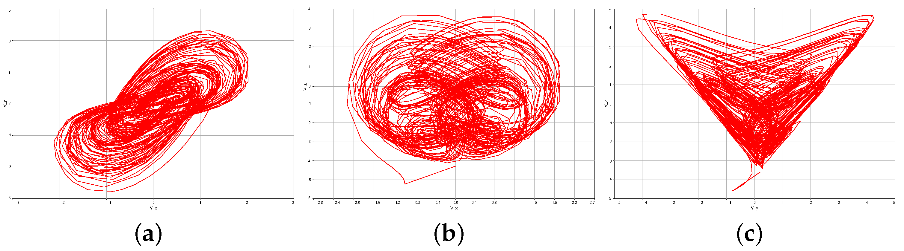
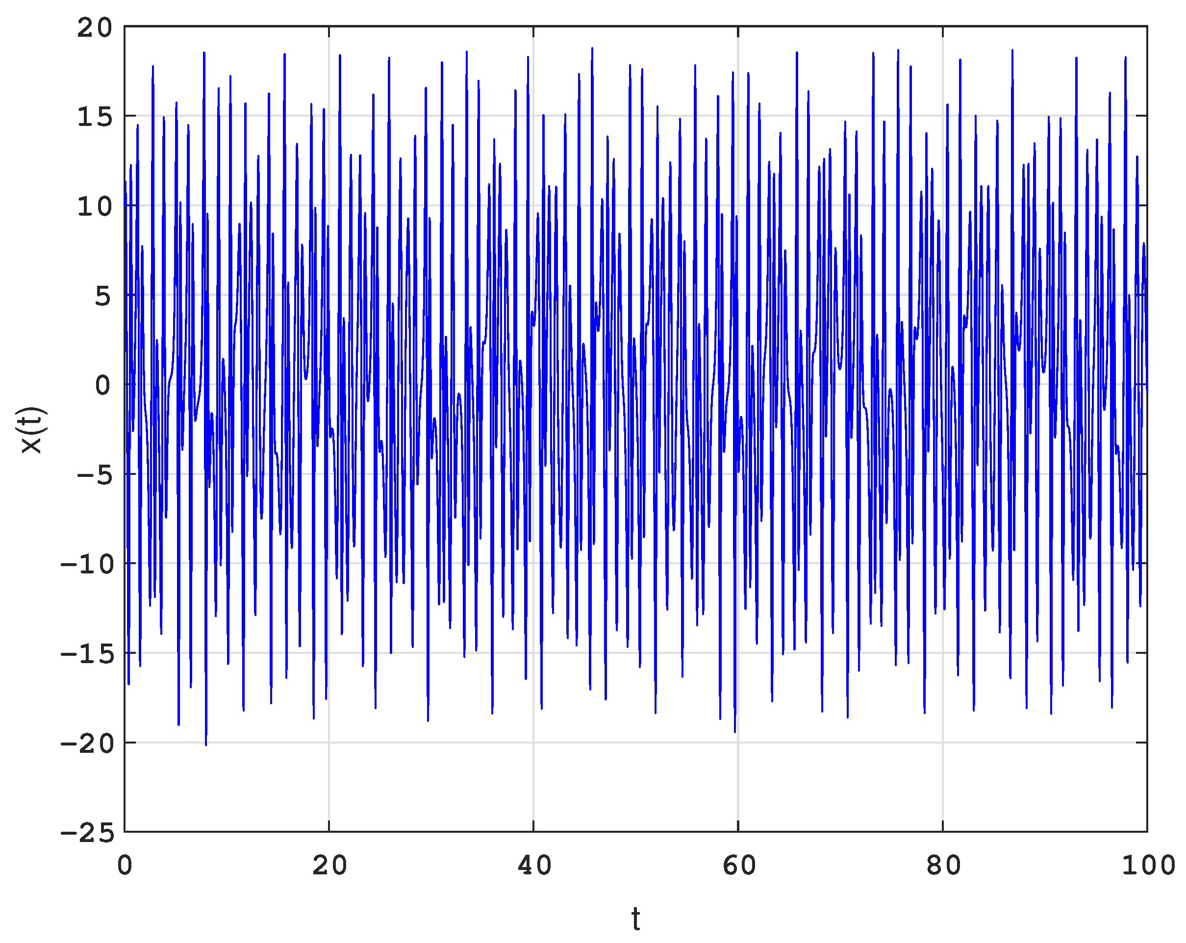
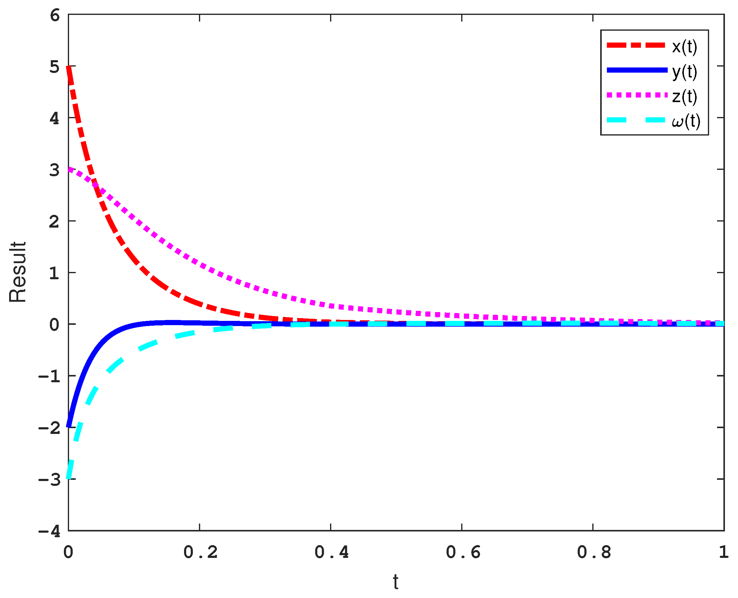
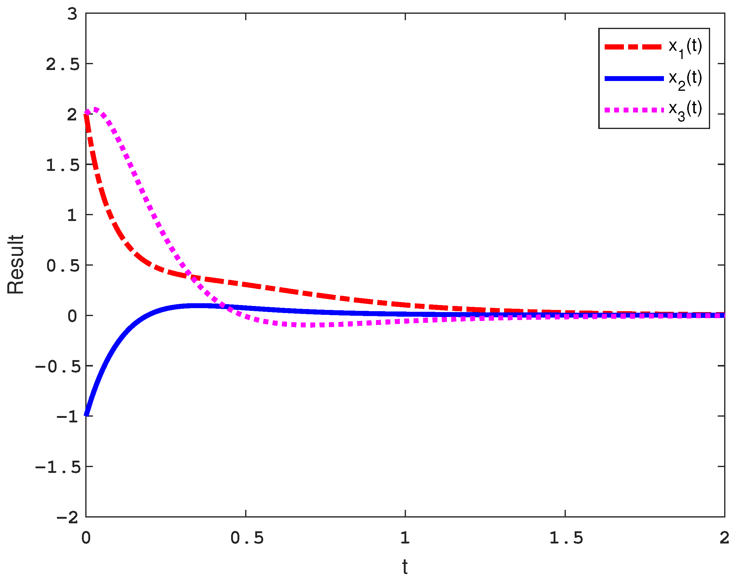
5. Numerical Simulation Examples

To enhance the persuasiveness of the method, two numerical simulation cases are used to illustrate the feasibility of the proposed method.

Example 1.

By analyzing of Section 3, system (5) of Section 2 can be described as

$$\stackrel{·}{\mathbf{x}}=B\mathbf{x}+Cf\left(\mathbf{x}\right),$$

(26)

in which

$$\mathbf{x}=\left[\begin{array}{c}x\\ y\\ z\\ \omega \end{array}\right],B=\left[\begin{array}{cccc}10& -10& 0& 0\\ 0& -22& 0& 1\\ 0& 0& -4& 0\\ 0& 4& 0& 0\end{array}\right],$$

$$C=\left[\begin{array}{cccc}0& 0& 0& 0\\ 1& 0& 0& 0\\ 0& 1& 1& 0\\ 0& 0& 0& 1\end{array}\right],f\left(\mathbf{x}\right)=\left[\begin{array}{c}xz\\ x^2\\ xy\\ 4x+0.5x^3\end{array}\right].$$

Suppose that $x\left(t\right)\in \left[-\xi ,\xi \right]$, where $\xi >0$ is a constant, then the following result is obtained

$$\begin{array}{c}{\parallel f\left(\mathbf{x}\right)\parallel }^2=0.25x^6+5x^4+16x^2+x^2{y}^2+x^2{z}^2\\ \le \left(0.25{\xi }^4+5{\xi }^2+16\right)x^2+{\xi }^2{y}^2+{\xi }^2{z}^2.\end{array}$$

Let $\mathbf{x}\left(0\right)={\left[5,-2,3,-3\right]}^T$, as shown in Figure 6, it can be obtained that $\left|x\left(t\right)\right|\le 21$, then

$$L=\mathit{diag}\left(0.25{\xi }^4+5{\xi }^2+16,{\xi }^2,{\xi }^2,0\right).$$

Choosing

$$K=\mathit{diag}\left(-2,-2,-2,-2\right).$$

Suppose that $T=0.4,d=0.0004$, by solving LMIs (24), (25), and inequality $p_1\ge p_2$, the following set of feasible solutions are obtained:

$${\mu }_1=45.60,{\mu }_2=45.60,p_1=90.85,p_2=90.75,$$

and

$$Q=\left[\begin{array}{cccc}50.0651& 4.5544& -0.4153& 0.8041\\ 4.5544& 2.7229& 0.0091& -0.2918\\ -0.4153& 0.0091& 1.4121& -1.3924\\ 0.8041& -0.2918& -1.3924& 2.6683\end{array}\right].$$

Thus, by the results obtained above, it can be concluded that the validity of Theorem 1 is proven. Besides, the time response curves of the controlled system with periodically intermittent control with variable control width are shown in Figure 7.

Example 2.

The following is a classical Chua’s circuit [43]:

$$\left\{\begin{array}{c}{\dot{x}}_1={\beta }_1\left(-x_1+x_2-f\left(x_1\right)\right),\hfill \\ {\dot{x}}_2=x_1-x_2+x_3,\hfill \\ {\dot{x}}_3=-{\beta }_2{x}_2,\hfill \end{array}\right.$$

(27)

with the piecewise linear function $f\left(x_1\right)=g_2{x}_1+\frac{1}{2}\left(g_1-g_2\right)\left(\left|x_1+1\right|-\left|x_1-1\right|\right)$, in which ${\beta }_1=9.2156,{\beta }_2=15.9946,g_1=-1.24905,g_2=-0.75735.$ Figure 8 shows that Chua’s oscillator with the initial condition $\mathbf{x}\left(0\right)={\left[x_1\left(0\right),x_2\left(0\right),x_3\left(0\right)\right]}^T={\left[2,0.3,-0.5\right]}^T$ produces a chaotic phenomenon.

Similarly, system (27) is rewritten as the following form:

$$\stackrel{·}{\mathbf{x}}=B\mathbf{x}+Cf\left(\mathbf{x}\right)$$

in which

$$\mathbf{x}=\left[\begin{array}{c}{x}_1\\ x_2\\ x_3\end{array}\right],B=\left[\begin{array}{ccc}-{\beta }_1-{\beta }_1{g}_2& {\beta }_1& 0\\ 1& -1& 1\\ 0& -{\beta }_2& 0\end{array}\right],$$

$$C=\left[\begin{array}{ccc}1& 0& 0\\ 0& 1& 0\\ 0& 0& 1\end{array}\right],f\left(\mathbf{x}\right)=\left[\begin{array}{c}\frac{-{\beta }_1\left(g_1-g_2\right)\left(\left|x_1+1\right|-\left|x_1-1\right|\right)}{2}\\ 0\\ 0\end{array}\right].$$

In addition, it can be obtained that

$$\begin{array}{cc}\hfill {∥f\left(\mathbf{x}\right)∥}^2& =0.5{{\beta }_1}^2{\left(g_1-g_2\right)}^2\left[x_1^2+1-\left|x_1^2-1\right|\right]\hfill \\ \hfill & =\left\{\begin{array}{c}{{\beta }_1}^2{\left(g_1-g_2\right)}^2,x_1^2>1\\ {{\beta }_1}^2{\left(g_1-g_2\right)}^2{x}_1^2,x_1^2⩽1\end{array}\right.\hfill \\ \hfill & ⩽{{\beta }_1}^2{\left(g_1-g_2\right)}^2{x}_1^2.\hfill \end{array}$$

Let $\mathbf{x}\left(0\right)={\left[2,-1,2\right]}^T$, and it can be obtained that

$$L=\mathit{diag}\left({\left({\beta }_1\left(g_1-g_2\right)\right)}^2,0,0\right).$$

Choosing

$$K=\mathit{diag}\left(-6,-6,-6\right).$$

Suppose that $T=2$, $d=0.0008$, by solving LMIs (24), (25), and inequality $p_1\ge p_2$, the following set of feasible solutions are obtained:

$${\mu }_1=6.60,{\mu }_2=6.60,p_1=12.85,p_2=12.75,$$

and

$$Q=\left[\begin{array}{ccc}1.3787& -0.3165& 0.4814\\ -0.3165& 2.3103& 0.3683\\ 0.4814& 0.3683& 0.4668\end{array}\right].$$

Thus, by the results obtained above, it can be concluded that the validity of Theorem 1 is proven. Moreover, the time response curves of the controlled Chua’s oscillator with periodically intermittent control with variable control width is shown in Figure 9. Compared with the results in work [23], the proposed method reduces the time for the system to reach the stable state, and the value of K is also reduced.

6. Conclusions

In this paper, a memristor-based hyper-chaotic Bao-like system is established based on the three-dimensional Bao chaotic system, and its analog circuit is also designed, which is used to verify the chaotic behaviors of the system. Furthermore, the periodically intermittent control method with variable control width is proposed, and the method is used to control the proposed system and the Chua’s oscillator. Compared with the chaotic system, the hyper-chaotic system has more complex fundamental dynamics characteristics which can be used in secure communication. Therefore, our future work is to apply the designed hyper-chaotic system to secure communication.

References

1. Lorenz, E.N. Deterministic nonperiodic flow. J. Atmos. Sci. 1963, 20, 130–141. [Google Scholar] [CrossRef]
2. Bao, B.; Liu, Z.; Xu, J. New chaotic system and its hyperchaos generation. J. Syst. Eng. Electron. 2009, 20, 1179–1187. [Google Scholar] [CrossRef]
3. Lü, J.; Chen, G. A new chaotic attractor coined. Int. J. Bifurc. Chaos 2002, 12, 659–661. [Google Scholar] [CrossRef] [Green Version]
4. Cang, S.; Qi, G.; Chen, Z. A four-wing hyper-chaotic attractor and transient chaos generated from a new 4-D quadratic autonomous system. Nonlinear Dynam. 2010, 59, 515–527. [Google Scholar] [CrossRef]
5. Cang, S.; Chen, Z.; Wu, W. Circuit implementation and multiform intermittency in a hyper-chaotic model extended from the Lorenz system. Chin. Phys. B 2009, 18, 1792–1800. [Google Scholar] [CrossRef]
6. Chua, L.O. Memristor-the missing circuit element. IEEE Trans. Circuit Theory 1971, 18, 507–519. [Google Scholar] [CrossRef]
7. Strukov, D.B.; Snider, G.S.; Stewart, D.R.; Williams, R.S. The missing memristor found. Nature 2008, 459, 80–83. [Google Scholar] [CrossRef] [PubMed]
8. Sahin, M.E.; Taskiran, Z.G.; Guler, H.; Hamamci, S.E. Simulation and implementation of memristive chaotic system and its application for communication systems. Sens. Actuators A Phys. 2019, 290, 107–118. [Google Scholar] [CrossRef]
9. Borghetti, J.; Snider, S.G.; Kuekes, P.J.; Yang, J.J.; Stewart, D.R.; Williams, S.R. ‘Memristive’ switches enable ‘stateful’ logic operations via material implication. Nature 2010, 464, 873–876. [Google Scholar] [CrossRef] [PubMed]
10. Pershin, Y.V.; Massimiliano, D.V. Experimental demonstration of associative memory with memristive neural networks. Neural Netw. 2010, 23, 881–886. [Google Scholar] [CrossRef] [PubMed] [Green Version]
11. Pershin, Y.V.; Steven, L.F.; Massimiliano, D.V. Memristive model of amoeba learning. Phys. Rev. E 2009, 42, 021926. [Google Scholar] [CrossRef] [PubMed] [Green Version]
12. Driscoll, T.; Pershin, Y.V.; Basov, D.N.; Di Ventra, M. Chaotic memristor. Appl. Phys. A 2011, 102, 885–889. [Google Scholar] [CrossRef] [Green Version]
13. Ostrovskii, V.; Fedoseev, P.; Bobrova, Y.L.; Butusov, D. Structural and parametric identification of knowm memristors. Nanomaterials 2022, 12, 63. [Google Scholar] [CrossRef] [PubMed]
14. Itoh, M.; Chua, L.O. Memristor oscillators. Int. J. Bifurc. Chaos 2008, 13, 3183–3206. [Google Scholar] [CrossRef]
15. Min, G.; Wang, L.; Duan, S. A novel four-dimensional memristive hyperchaotic system with its analog circuit implementation. In Proceedings of the 12th International Symposium on Neural Networks, Jeju, Republic of Korea, 15–18 October 2015; pp. 157–165. [Google Scholar] [CrossRef]
16. Muthuswamy, B. Implementing memristor based chaotic circuits. Int. J. Bifurc. Chaos 2010, 20, 1335–1350. [Google Scholar] [CrossRef]
17. Xie, X.; Wen, S.; Feng, Y.; Onasanya, B.O. Three-stage-impulse control of memristor-based chen hyper-chaotic system. Mathematics 2022, 10, 4560. [Google Scholar] [CrossRef]
18. Yang, X.; Yang, Z.; Nie, X. Exponential synchronization of discontinuous chaotic systems via delayed impulsive control and its application to secure communication. Commun. Nonlinear Sci. 2014, 19, 1529–1543. [Google Scholar] [CrossRef]
19. Rao, R.; Lin, Z.; Ai, X.; Wu, J. Synchronization of epidemic systems with neumann boundary value under delayed impulse. Mathematics 2020, 10, 2064. [Google Scholar] [CrossRef]
20. Wu, K.; Onasanya, B.O.; Cao, L.; Feng, Y. Impulsive control of some types of nonlinear systems using a set of uncertain control matrices. Mathematics 2023, 11, 421. [Google Scholar] [CrossRef]
21. Chen, H.; Chen, J.; Qu, D.; Li, K.; Lou, F. An uncertain sandwich impulsive control system with impulsive time windows. Mathematics 2022, 10, 4708. [Google Scholar] [CrossRef]
22. Liao, C.; Tu, D.; Feng, Y.; Zhang, W.; Wang, Z.; Onasanya, B.O. A sandwich control system with dual stochastic impulses. IEEE/CAA J. Autom. Sin. 2022, 4, 741–744. [Google Scholar] [CrossRef]
23. Li, C.; Feng, G.; Lia, X. Stabilization of nonlinear systems via periodically intermittent control. IEEE Trans. Circuits Syst. 2007, 54, 1019–1023. [Google Scholar] [CrossRef]
24. Li, C.; Liao, X.; Huang, T. Exponential stabilization of chaotic systems with delay by periodically intermittent contro. Chaos 2007, 17, 013103. [Google Scholar] [CrossRef]
25. Ding, K.; Zhu, Q. Intermittent extended dissipative control for delayed distributed parameter systems with stochastic disturbance: A spatial point sampling approach. IEEE Trans. Fuzzy Syst. 2020, 30, 1734–1749. [Google Scholar] [CrossRef]
26. Ding, K.; Zhu, Q.; Li, H. A generalized system approach to intermittent nonfragile control of stochastic neutral time-varying delay systems. IEEE Trans. Syst. Man Cybern. Syst. 2021, 51, 7017–7026. [Google Scholar] [CrossRef]
27. Liu, B.; Liu, T.; Xiao, P. Dynamic event-triggered intermittent control for stabilization of delayed dynamical systems. Automatica 2023, 149, 110847. [Google Scholar] [CrossRef]
28. Zhou, H.; Chen, Y.; Chu, D.; Li, W. Impulsive stabilization of complex-valued stochastic complex networks via periodic self-triggered intermittent control. Nonlinear Anal. Hybrid Syst. 2023, 48, 101304. [Google Scholar] [CrossRef]
29. Zhang, Z.; He, Y.; Zhang, Y.; Wu, M. Exponential stabilization of neural networks with time-varying delay by periodically intermittent control. Neurocomputing 2016, 207, 469–475. [Google Scholar] [CrossRef]
30. Wang, Q.; He, Y.; Tan, G.; Wu, M. Observer-based periodically intermittent control for linear systems via piecewise Lyapunov function method. Appl. Math. Comput. 2017, 293, 438–447. [Google Scholar] [CrossRef] [Green Version]
31. Wang, Y.; He, Y. Fuzzy synchronization of chaotic systems via intermittent control. Chaos 2018, 106, 154–160. [Google Scholar] [CrossRef]
32. You, L.; Yang, X.; Wu, S.; Li, X. Finite-time stabilization for uncertain nonlinear systems with impulsive disturbance via aperiodic intermittent control. Appl. Math. Comput. 2023, 443, 127782. [Google Scholar] [CrossRef]
33. Xu, C.; Tong, D.; Chen, Q.; Zhou, W.; Xu, Y. Exponential synchronization of chaotic systems with stochastic noise via periodically intermittent control. Int. J. Robust Nonlinear Control 2020, 30, 2611–2624. [Google Scholar] [CrossRef]
34. Yang, X.; Feng, Y.; Yiu, K.F.C.; Song, Q.; Alsaadi, F.E. Synchronization of coupled neural networks with infinite-time distributed delays via quantized intermittent pinning control. Nonlinear Dynam. 2018, 94, 2289–2303. [Google Scholar] [CrossRef]
35. Ding, K.; Zhu, Q.; Huang, T. Prefixed-time local intermittent sampling synchronization of stochastic multicoupling delay reaction-diffusion dynamic networks. IEEE Trans. Neural Netw. Learn. Syst. 2022, 16, 1–15. [Google Scholar] [CrossRef]
36. Gabelli, J.; Fve, G.; Berroir, B.; Etienne, B.; Glattli, D. Violation of Kirchhoff’s Laws for a Coherent RC Circuit. Science 2006, 313, 499–502. [Google Scholar] [CrossRef] [Green Version]
37. Bao, B.; Liu, Z.; Xu, T. Steady periodic memristor oscillator with transient chaotic behaviours. Electron. Lett. 2010, 46, 237–238. [Google Scholar] [CrossRef]
38. Wolf, A.; Swift, J.B.; Swinney, H.L.; Vastano, J.A. Determining Lyapunov exponents from a time series. Physica D 1985, 16, 285–317. [Google Scholar] [CrossRef] [Green Version]
39. Shaw, R. Strange attractors, chaotic behavior, and information flow. Z. Naturforsch. A 1981, 36, 80–112. [Google Scholar] [CrossRef]
40. Frederickson, P.; Kaplan, J.L.; Yorke, E.D.; Yorke, J.A. The Liapunov dimension of strange attractors. J. Differ. Equ. 1983, 49, 185–207. [Google Scholar] [CrossRef] [Green Version]
41. Sanchez, E.N.; Perez, J.P. Input-to-state stability (ISS) analysis for dynamic neural networks. IEEE Trans. Circuits Syst. 1999, 46, 1395–1398. [Google Scholar] [CrossRef]
42. Boyd, S.; Ghaoui, L.; Feron, E.E.; Balakrishnan, V. Linear Matrix Inequalities in System and Control Theory. Chaos Soliton Fractals 1994, 15, 157–193. [Google Scholar] [CrossRef]
43. Shil’nikov, L.P. Chua’s circuit: Rigorous results and future problems. Int. J. Bifurc. Chaos 1994, 4, 489–519. [Google Scholar] [CrossRef]
Figure 1. Circuit implementation diagram of Bao chaotic system.
Mathematics 11 01264 g001
Figure 2. Chaotic attractor phase diagram for the hyper-chaotic Bao-like system based on memristor with the initial condition x 0 = 10 , 10 , 10 , 10 T . (a) x-y- ω plane. (b) x-y plane. (c) x-z plane. (d) y-z plane.
Mathematics 11 01264 g002
Figure 3. The Lyapunov exponential spectrum of the memristor-based hyper-chaotic Bao-like system with the initial condition x 0 = 10 , 10 , 10 , 10 T .
Mathematics 11 01264 g003
Figure 4. Circuit implementation diagram of the memristor-based hyper-chaotic Bao-like system.
Mathematics 11 01264 g004
Figure 5. Chaotic attractor phase diagram for the hyper-chaotic Bao-like system based on memristor with the initial condition x 0 = 1 , 1 , 1 , 1 T . (a) x-y plane. (b) x-z plane. (c) y-z plane.
Mathematics 11 01264 g005
Figure 6. Time diagram of state variable x with the initial condition x 0 = 5 , 2 , 3 , 3 T .
Mathematics 11 01264 g006
Figure 7. The time response curves of the controlled system with periodically intermittent control with variable control width.
Mathematics 11 01264 g007
Figure 8. Chua’s oscillator produces a chaotic phenomenon with the initial condition x 0 = 2 , 0.3 , 0.5 T .
Mathematics 11 01264 g008
Figure 9. The time response curves of the controlled Chua’s oscillator with periodically intermittent control with variable control width.
Mathematics 11 01264 g009