A Systematic Review on the Solution Methodology of Singularly Perturbed Differential Difference Equations

Abstract

This review paper contains computational methods or solution methodologies for singularly perturbed differential difference equations with negative and/or positive shifts in a spatial variable. This survey limits its coverage to singular perturbation equations arising in the modeling of neuronal activity and the methods developed by numerous researchers between 2012 and 2022. The review covered singularly perturbed ordinary delay differential equations with small or large negative shift(s), singularly perturbed ordinary differential–differential equations with mixed shift(s), singularly perturbed delay partial differential equations with small or large negative shift(s) and singularly perturbed partial differential–difference equations of the mixed type. The main aim of this review is to find out what numerical and asymptotic methods were developed in the last ten years to solve such problems. Further, it aims to stimulate researchers to develop new robust methods for solving families of the problems under consideration.

1. Background of the Problem

Many scientific problems describe the relations between causes and their effects. The study of this relation in the subject of the perturbations theory has a long history [1]. Despite this long history, the topic is still in a state of irrepressible development and is termed as the theory of singular perturbation problems (SPPs). The SPPs containing a small parameter value (say $\epsilon$), where $0<\epsilon \ll 1$ received remarkable attention from mathematicians and physicists. Scholars working on the solution methodologies of SPPs have carried out numerous studies and reviews. A survey on the asymptotic and numerical methods for solving SPPs was conducted by [2]. In 2002, ref. [3] reviewed the work of numerous researchers in SPPs from 1984 to 2000. Ref. [4] reviewed solution methodology for singularly perturbed partial differential equations. Ref. [5] carried out a survey on computational techniques for solving singularly perturbed boundary value problems. Ref. [6] briefly reviewed the computational methods developed to solve various classes of SPPs. Ref. [7] reviewed the development of computational methods for solving singularly perturbed (SP) boundary value problems. Ref. [8] discussed the numerical analysis of singularly perturbed convection–diffusion–reaction problems that appeared in 2008–2012, mainly focused on layer-adapted meshes. Ref. [9] reviewed singularly perturbed differential equations with turning point and interior layers. Ref. [10] discussed the review of singularly perturbed delay differential equations. This systematic review briefly assesses the solution methodologies on singularly perturbed differential–difference equations (SPDDEs).

The differential equations in which the highest order derivative is multiplied by a small positive parameter and contains a delay parameter (negative shift) and/or advance parameter (positive shift) is known as a singularly perturbed differential–difference equation (SPDDE). Such problems frequently arise in modeling biosciences, vibrational models in control theory, physiological processes, diseases, economics, engineering, and so on. A few application fields are the mathematical modeling of population dynamics [11], immune response [12], variational problem in control theory [13,14], model of HIV infection [15,16,17], activation of neuronal variability [17,18], modeling of biological oscillators [19], mathematical ecology [20], models for physiological processes [21,22], evolutionary biology [23], neuronal variability [24], and others.

Due to the dual presence of singular perturbation ($\epsilon$) and shift arguments in the SPDDEs, it is very difficult to obtain oscillation-free solutions on a uniform mesh unless using specially designed meshes. A thoughtful examination of the results from the conventional numerical methods, such as the finite difference method (FDM), the finite element method (FEM), the finite volume method(FVM), the spline method, and other methods, on uniform meshes as $\epsilon \to 0$ fails for a satisfactory numerical solution, and the truncation error becomes unbounded unless a large number of mesh points or adaptive layer mesh is used in the approximation process [25]. This shows that the classical numerical method is computationally costly and inefficient. Sometimes, the increase in mesh points also causes the resulting systems of algebraic equations to be ill-conditioned. This drawback motivates researchers to develop robust numerical methods for SPDDEs. In this context, the fitted operator method (FOM) and fitted mesh method (FMM) are popular techniques to overcome the drawbacks of classical numerical methods. For more details about FOMs and FMMs, refer to the books and articles [18,25,26,27] and the references therein.

In this review, we investigate the solution methodology for the class of singularly perturbed delay ordinary differential equations (SPDODEs) with small or large negative shift(s), singularly perturbed ordinary differential–differential equations (SPODDEs) with mixed shift(s), singularly perturbed delay partial differential equations(SPDPDEs) with small or large negative shift(s), and singularly perturbed partial differential–difference equations (SPPPDDEs) of the mixed type that were solved from 2012 to 2022 using different numerical and asymptotic methods.

2. Models Depicting Singular Perturbation of Difference–Differential Problems

Several real-life problems are described by singularly perturbed differential–difference with mixed shifts of which the following are the major ones to consider for this particular study.

2.1. The Modeling of the Activation of a Neuron [28]

The authors in [28] generalized the Stein’s model in terms of SPODDEs to consider the time evolution trajectories of the membrane potential:

$$\begin{array}{c}\frac{{\gamma }^2}{2}{u}^{″}\left(x\right)+\left(\lambda -x\right)u^{″}\left(x\right)+{\sigma }_{e}u(x+a_e)+{\sigma }_{i}u(x-a_i-\left({\sigma }_e+{\sigma }_i\right)u\left(x\right)=-1,\hfill \end{array}$$

subject to the boundary conditions:

$$\begin{array}{c}u\left(x\right)=0,x\notin (x_1,x_2),\hfill \end{array}$$

where the values $x=x_1$ and $x=x_2$ relate to the inhibitory reversal potential and to the threshold value of membrane potential for action potential generation, respectively, and to the non-derivative terms related to excitatory and inhibitory synaptic inputs.

2.2. Neuronal Variability [29]

The authors in [29] generalized the Stein’s model and proposed the following mathematical model in terms of SPPPDDEs to consider the time evolution trajectories of the membrane potential:

$$-\frac{\partial z}{\partial t}=\frac{{\gamma }^2}{2}\frac{{\partial }^{2}z}{\partial x^2}+(\sigma D-\frac{x}{\lambda })\frac{\partial z}{\partial x}+{\tau }_{s}z(x+a_s,t)+w_{s}z(x+i_s,t)-({\tau }_s+w_s)z(x,t),$$

where the non-derivative terms are allied to the superposition of excitatory and inhibitory inputs.

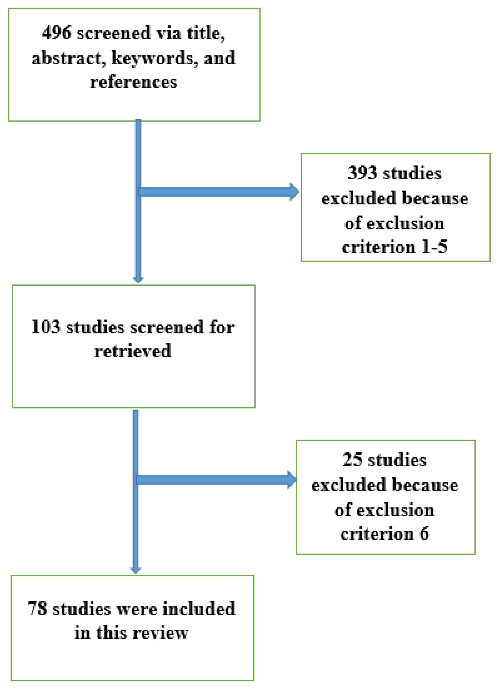
3. Criteria for Including Studies and Selection Procedure

3.1. Literature Search

The relevant studies were identified by the use of electronic databases: Web of Science, SCOPUS, and PubMed. In addition, the relevant articles were collected from different Internet sources via Google Scholar, ResearchGate, and Sci-hub, library genius. Whenever possible, search organizers were used to align the initial survey results more thoroughly with the eligibility criteria. For example, studies written in English and published on SCOPUS/Web of Science (SCIE/SSCI) indexed journals during the years 2012 to 2022 were included. The search was completed in 30 January 2022.

3.2. Screening Process

Electronic and manual searches identified 496 potentially relevant studies and screened for retrieval via title, abstract, keywords, and references. Then, 78 studies included in this review were screened according to the screening criteria given in

Table 1. Inclusion and exclusion criteria of studies included in the review.

Criterion	Include	Exclude
1. Studies focusing on	SPODDEs with small or large delay,	SPODDEs without shift(s)
	small mixed shifts and small delays
2. Studies focusing on	SPPPDDEs with small or large delay,	SPPPDDEs without shift(s)
	small mixed shifts and small delays
3. Boundary conditions	Dirichlet BC	Non-Dirichlet BC
4. Publication year	2012–2022	Before 2012
5. Language	English	Non-English
6. Indexed	on SCOPUS/Web of science	not SCOPUS/Web of science
	/PubMed	/PubMed

. Figure 1 shows various steps in the process of selecting studies and depicting how we ended up with the 78 original studies we further analyzed.

4. Developments toward Solution Methodology for SPDDEs

In this paper, we discuss a survey in chronological order on the asymptotic and numerical treatment of SPDDEs of both ordinary and partial differential equations. For the sake of convenience, we divide this survey into twelve parts chronologically. We would like to apologize if there are any omissions, which are totally unintentional.

4.1. Developments toward Solution Methodology for SPODDEs

In this subsection, we give a brief description of the developed numerical methods for SPODDE of the form on the domain $D=(-1,1)$:

$$\begin{array}{c}-{\epsilon }^2\frac{d^{2}u\left(x\right)}{d{x}^2}+a\left(x\right)\frac{du\left(x\right)}{dx}+b\left(x\right)u(x-\delta )+c\left(x\right)u(x,)+d\left(x\right)u(x+\eta )=f\left(x\right),x\in D,\hfill \end{array}$$

(1)

subject to the following interval boundary conditions (IBCs):

$$\begin{array}{c}u\left(x\right)={\varsigma }_1\left(x\right),x\in \left[-\delta ,0\right],\hfill \\ u\left(x\right)={\varsigma }_2\left(x\right),x\in \left[1,1+\eta \right],\hfill \end{array}$$

(2)

where $0<\epsilon \ll 1$ is a singular perturbation parameter, $\delta$ is delay, and $\eta$ is an advance parameter satisfying either $\delta ,\eta \le \epsilon$ or $\delta ,\eta \ge \epsilon$. For the existence and uniqueness of the solution, the functions $a\left(x\right),b\left(x\right),c\left(x\right),d\left(x\right)$, $u\left(x\right),{\varsigma }_1\left(x\right)$, and ${\varsigma }_2\left(x\right)$ are assumed to be sufficiently smooth and bounded with $b\left(x\right)+c\left(x\right)+d\left(x\right)\ge \theta >0\mathrm{for}\mathrm{all}x\in \overline{D}$ and for some positive constant $\theta$.

As can be seen from

Table 2. Various methods and mesh used to solve Equations (1) and (2).

Author(s)	Solution Methodology	Meshes
[34]	Exponentially fitted FDM based on Il’in-Allen-Southwell fitting	Specially designed mesh
[30]	Fitted modified upwind finite difference method	Uniform mesh
[35]	Collocation in combination with matrices of Fibonacci polynomials	Uniform mesh
[36]	Domain decomposition method	Uniform mesh
[37]	Asymptotic-numerical method	Uniform mesh
[38]	Fitted non-standard finite difference method	Uniform mesh
[39]	Galerkin method with exponential fitting	Uniform mesh
[40]	Fourth order finite difference method	Uniform mesh
[41]	Mixed FDM via domain decomposition	Uniform mesh
[42]	New exponentially fitted three term finite difference scheme	Uniform mesh
[43]	Fourth-order Runge–Kutta method	Uniform mesh
[44]	Numerical integration scheme using non polynomial interpolation function	Uniform mesh
[45]	Exponentially fitted non-standard FDM	Uniform mesh
[46]	Exponentially fitted operator finite difference method with Richardson extrapolation	Uniform mesh
[47]	Hybrid of the midpoint upwind FDM and the central FDM	Piecewise uniform Shishkin mesh
[31]	Hybrid finite difference scheme with the cubic spline	Piecewise uniform Shishkin mesh

and

Table 3. Various methods and mesh used to solve Equations (1) and (2).

Author(s)	Solution Methodology	Meshes
[32]	FDM	Uniform mesh
[48]	Finite element method	Bakhvalov-S-mesh
[33]	Non-standard FDM	Uniform mesh
[49]	Finite difference approach with a parametric spline	Uniform mesh
[50]	Fitted non-polynomial spline approach	Uniform mesh
[51]	Successive complementary expansion method (SCEM)	Uniform mesh
[52]	Haar wavelet collocation method	Uniform mesh

, most of the solution methodologies presented to solve problems (1) and (2) were developed based on uniform mesh except for three works presented by [30,31,32,33]. Further, the majority of the methods are finite-difference-based. This implies that it is possible to think of other alternative techniques to solve the governing equation of the problem under consideration on either uniform or adaptive mesh discretization techniques.

4.2. Developments toward Solution Methodology for SP Convection Diffusion Problem with Large Shift in Space

In this subsection, we want to look at the static SPP given by

$$\begin{array}{c}-\epsilon \frac{d^{2}u\left(x\right)}{d{x}^2}-b\left(x\right)\frac{du\left(x\right)}{dx}+c\left(x\right)u\left(x\right)+d\left(x\right)u(x-1)=f\left(x\right),x\in (0,2),\end{array}$$

(3)

subject to the following boundary conditions (BCs):

$$\begin{array}{c}u\left(2\right)=0,u\left(x\right)=\varphi \left(x\right),x\in (-1,0],\end{array}$$

(4)

where $0<\epsilon \ll 1$, $b\left(x\right)\ge \beta >0,d\ge 0,c-\frac{b^{\prime }{L}_{\infty }(1,2)}{2}\ge \gamma >0$.

The results in

Table 4. Various methods and mesh used to solve Equations (3) and (4).

Author(s)	Solution Methodology	Meshes
[53]	Asymptotic initial value technique (AIVT)	Piece-wise uniform Shishkin mesh
[54]	Exponentially fitted FDM	Uniform mesh
[55]	Fourth FDM	Uniform mesh
[56]	Cubic spline in compression method	Uniform mesh

reveal that all the methods developed to solve the problem under consideration in Equations (3) and (4) followed a uniform mesh discretization approach. However, only scholars in [53] applied the nonuniform or adaptive mesh approach, particularly the Shshikin mesh technique. It is also observable from the results in the table that very few methods have been developed to solve the problem under consideration in Equations (3) and (4). Hence, the solution methodology development for the problem is at its infant stage.

4.3. Developments toward Solution Methodology for SP Reaction Diffusion Problem with Large Shift in Space

In this subsection, we want to look at the static SPP given by

$$\begin{array}{c}-{\epsilon }^2\frac{d^{2}u\left(x\right)}{d{x}^2}+a\left(x\right)u\left(x\right)+b\left(x\right)u(x-1)=f\left(x\right),x\in (0,2),\hfill \end{array}$$

(5)

with IBCs:

$$u\left(2\right)=L,u\left(x\right)=\varphi \left(x\right),x\in (-1,0],$$

(6)

where $0<\epsilon \ll 1$, $a\left(x\right)\ge \alpha >0,{\beta }_0\le b\left(x\right)\le \beta <0,\alpha +{\beta }_0\ge \eta >0,\forall x\in [0,2]$.

The results presented in

Table 5. Various methods and mesh used to solve Equations (5) and (6).

Author(s)	Solution Methodology	Meshes
[57]	Non-symmetric discontinuous Galerkin FEM	Shishkin polynomial Shishkin(pS) Bakhvalov–Shishkin (BS) modified Bakhvalov–Shishkin (mBS-) mesh
[58]	Hybrid finite difference scheme	Piece-wise uniform Shishkin mesh
[59]	Exponentially fitted numerical scheme via domain decomposition	Uniform mesh
[60]	Classical FDM	Piece-wise uniform Shishkin mesh
[61]	Numerov FDM	Uniform mesh
[62]	Iterative method	Shishkin mesh and Bakhvalov Shishkin mesh (BS mesh).
[63]	Numerov method	Uniform Mesh.
[64]	Central FDM	Uniform Mesh.

belong to the solution methodologies developed for Equations (5) and (6). It reveals that most numerical methods developed were based on nonuniform discretization techniques, namely Shihikin-, Bakhavlov-, and Shishkin–Bakhavlov-type discretization techniques. Furthermore, all the methods developed are based on finite difference approximation techniques except [57], a finite element method.

4.4. Developments toward Solution Methodology for SP Reaction Diffusion Problem with Small Shift

In this subsection, we want to look at the static SPP given by

$$\begin{array}{c}-\epsilon \frac{d^{2}u\left(x\right)}{d{x}^2}+a\left(x\right)u(x-\delta )+b\left(x\right)u\left(x\right)=f\left(x\right),x\in (0,1),\hfill \end{array}$$

(7)

subject to the following IBCs:

$$u\left(1\right)=L,u\left(x\right)=\varphi \left(x\right),-\delta \le x\le 0.$$

(8)

Table 6. Various methods and mesh used to solve Equations (7) and (8).

Author(s)	Solution Methodology	Meshes
[65]	Non-polynomial cubic spline method	Uniform mesh
[55]	Fourth FDM	Uniform mesh
[66]	Fourth order exponentially FDM	Uniform mesh
[67]	Trapezoidal rule	Uniform mesh
[68]	Simpson rule	Uniform mesh

consists of the results of the solution methodology developed for the SP reaction–diffusion problem given in Equations (7) and (8). As can be seen from the review result, very few numerical methods have been developed to solve the problems described by the governing Equations (7) and (8), and they are all based on uniform discretization techniques. The methods are mainly finite difference methods and numerical integration techniques. Hence, one can look for finite elements and other quadrature techniques based on adaptive mesh approaches.

4.5. Developments toward Solution Methodology for SP Convection Diffusion Problem with Negative Shift

In this subsection, we review numerical schemes developed for SPP given by

$$\begin{array}{c}-\epsilon \frac{d^{2}u\left(x\right)}{d{x}^2}+a\left(x\right)\frac{du\left(x-\delta \right)}{dx}+b\left(x\right)u\left(x\right)=f\left(x\right),x\in (0,1),\hfill \end{array}$$

(9)

with IBCs:

$$\begin{array}{c}u\left(1\right)=A,u\left(x\right)=\psi \left(x\right),-\delta \le x\le 0.\hfill \end{array}$$

(10)

Table 7. Various methods and mesh used to solve Equations (9) and (10).

Author(s)	Solution Methodology	Meshes
[69]	Exponential spline method	Uniform mesh
[70]	Non-polynomial spline method	Uniform mesh
[71]	Novel FDM	Uniform mesh

reveals that only a few finite-difference-based solution methodologies on a uniform mesh discretization approach were generally developed to solve the problem of the family of SPDDEs described by the governing equation in (9) and (10). This implies that this area needs the attention of scholars working in this and related research areas.

4.6. Developments toward Solution Methodology for SP Convection Diffusion Problem with Negative Shift

In this subsection, we want to look at the static SPP given by

$$\begin{array}{c}-\epsilon \frac{d^{2}u\left(x\right)}{d{x}^2}+a\left(x\right)\frac{du\left(x\right)}{dx}+b\left(x\right)u(x-\delta )=f\left(x\right),x\in (0,1),\hfill \end{array}$$

(11)

with IBCs:

$$\begin{array}{c}u\left(1\right)=\beta ,u\left(x\right)=\varphi \left(x\right),-\delta \le x\le 0.\hfill \end{array}$$

(12)

As seen from

Table 8. Various methods and mesh used to solve Equations (11) and (12).

Author(s)	Solution Methodology	Meshes
[72]	Tension splines method	Uniform mesh
[73]	New Liouville–Green Transform method	Uniform mesh
[74]	Exponentially fitted spline method	Uniform mesh
[75]	Exponentially fitted FDM	Equidistant mesh

, the family of SP problems described by the governing equation in (11) and (12) is solved by using various numerical methods, namely fitted operator finite difference methods, spline intention methods, and new Lioville–Green transform methods. Furthermore, all the techniques were developed based on uniform mesh discretization techniques. Like others, finite element approaches and adaptive mesh techniques can be considered an alternative to solve the problem.

4.7. Developments toward Solution Methodology for SPODDE with Negative Shifts

In this subsection, we give a brief description of the developed numerical methods for SPODDE of the form:

$$\begin{array}{c}-\epsilon \frac{d^{2}u\left(x\right)}{d{x}^2}+a\left(x\right)\frac{du\left(x-\delta \right)}{dx}+b\left(x\right)u(x-\delta )+c\left(x\right)u\left(x\right)=f\left(x\right),x\in (0,1),\hfill \end{array}$$

(13)

subject to IBCs:

$$\begin{array}{c}u\left(x\right)=\varphi \left(x\right),x\in [-\delta ,0],u\left(1\right)=\psi \left(1\right).\hfill \end{array}$$

(14)

Table 9. Various methods and mesh used to solve Equations (13) and (14).

Author(s)	Solution Methodology	Meshes
[77]	Non-standard mid-point upwind FDM, Standard mid-point upwind FDM, Non-standard mid-point upwind FDM	Uniform mesh, Shiskin mesh, Shiskin mesh
[78]	Exponentially fitted operator Mid-point upwind FDM	Uniform mesh
[79]	Exponentially fitted upwind FDM with Richardson extrapolation technique	Uniform mesh
[80]	Central FDM	Uniform mesh
[76]	B-spline collocation method	Piecewise uniform Shishkin mesh

summarizes the solution methodologies developed to solve SP problems involving small negative shifts both in convection and reaction terms given in (13) and (14). Almost all the developed methods are the families of fitted operator finite difference methods except [76], the B-spline collocation method. In this case, the peculiarity is that some of the fitted operator methods are developed on layer adaptive meshes, which are unique approaches.

4.8. Developments toward Solution Methodology for SPPPDDEs with Mixed Shifts

In this subsection, we give a brief description of the developed numerical methods for SPPPDDE of the form on the domain $\Im ={\Im }_x\times {\Im }_t=(0,1)\times (0,T]$ for some fixed number $T>0$:

$$\begin{array}{c}\frac{\partial w\left(x,t\right)}{\partial t}-{\epsilon }^2\frac{{\partial }^{2}w\left(x,t\right)}{\partial x^2}+\omega \left(x\right)\frac{\partial w\left(x,t\right)}{\partial x}+\varpi \left(x\right)\zeta (x-\delta ,t)+\varrho \left(x\right)w(x,t)+\phi \left(x\right)w(x+\eta ,t)\hfill \\ =f(x,t),(x,t)\in \Im ,\hfill \end{array}$$

(15)

subject to the following initial interval boundary conditions (I-IBCs):

$$\begin{array}{c}w(x,0)=w_0\left(x\right),x\in {\overline{\Im }}_x,\hfill \\ w(x,t)=w_1(x,t),-\delta \le x\le 0,t\in (0,T],\hfill \\ w(x,t)=w_2(x,t),1\le x\le 1+\eta ,t\in (0,T],\hfill \end{array}$$

(16)

where $0<\epsilon \ll 1$, $\delta$ is the delay, and $\eta$ is the advance parameter satisfying either $\delta ,\eta \le \epsilon$ or $\delta ,\eta \ge \epsilon$.

Table 10. Various methods and mesh used to solve Equations (15) and (16).

	Numerical Scheme
Author(s)	Temporal Direction	Spatial Direction	Meshes
[87]	Implicit Euler method	FDM	Uniform mesh
[88]	Implicit Euler method	Non-standard FDM	Special type of mesh
[87]	Implicit Euler method	Combined FDM made out of modified upwind and central difference schemes	Uniform mesh
[89]	Crank–Nicolson FDM	Midpoint upwind FDM	Piecewise-uniform Shishkin mesh
[90]	Implicit Euler FDM	Hybrid of midpoint upwind FDM and classical central FDM	Piecewise-uniform Shishkin mesh
[91]	Backward Euler formula	Exponentially fitted FDMs	Uniform mesh
[92]	Implicit Runge–Kutta method	Non-standard FDM	Uniform mesh
[81]	Implicit Euler method	Extended cubic B-spline basis functions	Uniform mesh
[93]	Implicit Euler method	Exponentially fitted operator FDM	Uniform mesh
[94]	Backward Euler method	New FDM	Uniform mesh
[95]	Implicit Euler method	Central FDM	Uniform mesh

and

Table 11. Various Methods and Mesh used to solve Equations (15) and (16).

	Numerical Scheme
Author(s)	Temporal Direction	Spatial Direction	Meshes
[96]	Crank–Nicolson method	Quadratic B-spline collocation method	Exponentially graded
[82]	Implicit Euler method	Specially designed FDM	Uniform mesh
[97]	Implicit Euler method	Hybrid computational method consisting of midpoint upwind FDM and cubic spline in tension method	Piecewise-uniform Shishkin mesh
[83]	Crank–Nicolson method	Non-standard FDM	Uniform mesh
[84]	Crank–Nicolson method	Modified cubic B-spline basis functions	Shishkin mesh
[85]	Implicit Euler method	Cubic B-collocation method	Uniform mesh
[86]	Implicit Euler method	Cubic spline in tension method	Uniform mesh

summarize the solution methodologies for singularly perturbed families of partial differential–difference equations given in (15) and (16). The majority of the methods developed are mainly from the families of finite difference methods except for a few methods, namely [81,82,83,84,85,86]. From the point of view of the discretization techniques, almost all have used either the implicit Euler method or the Crank–Nicholson method for temporal discretization, whereas both uniform and nonuniform are used for spatial mesh discretization.

4.9. Developments toward Solution Methodology for SPDPDEs with Large Delay in Space

In this subsection, we give a brief description of the developed numerical methods for SPDPDEs of the form on the domain $D={\Omega }_x\times {\Omega }_t=(0,2)\times (0,T]$ for some fixed number $T>0$:

$$\begin{array}{c}\frac{\partial y\left(x,t\right)}{\partial t}-\epsilon \frac{{\partial }^{2}y\left(x,t\right)}{\partial x^2}+r\left(x\right)y(x,t)+s\left(x\right)y(x-1,t)=g(x,t),(x,t)\in D,\hfill \end{array}$$

(17)

subject to the following I-IBCs:

$$\begin{array}{c}y(x,0)=y_0\left(x\right),x\in {\overline{\Omega }}_x,\hfill \\ y(x,t)=\varphi (x,t),-1\le x\le 0,t\in (0,T],\hfill \\ y(2,t)=\psi (2,t),t\in (0,T].\hfill \end{array}$$

(18)

As can be seen from

Table 12. Various methods and mesh used to solve Equations (17) and (18).

	Numerical Scheme
Author(s)	Temporal Direction	Spatial Direction	Meshes
[98]	Implicit Euler method	Central FDM	Piecewise-uniform Shishkin mesh
[99]	Crank–Nicolson method	FDM	Piecewise-uniform Shishkin mesh
[100]	Discontinuous Galerkin method	$\beta$-weighted continuous Galerkin FEM	Duran- and S-type meshes

, only three types of solution methodologies have been developed for the SP reaction–diffusion partial differential equation with a large negative shift given by the governing equation in (17) and (18). All are designed on an adaptive mesh discretization approach which guarantees the parameter uniformity of the methods.

4.10. Developments toward Solution Methodology for SPDPDEs with Small Negative Shift in Space

In this subsection, we give a brief description of the developed numerical methods for SPDPDEs of the form on the domain $\Lambda ={\Gamma }_x\times {\Gamma }_t=(0,1)\times (0,T]$ for some fixed number $T>0$:

$$\begin{array}{c}\frac{\partial z\left(x,t\right)}{\partial t}-\epsilon \frac{{\partial }^{2}z\left(x,t\right)}{\partial x^2}+a\left(x\right)\frac{\partial z\left(x,t\right)}{\partial x}+r\left(x\right)z(x,t)+s\left(x\right)z(x-\delta ,t)=h(x,t),(x,t)\in \Lambda ,\hfill \end{array}$$

(19)

subject to the following I-IBCs:

$$\begin{array}{c}z(x,0)=z_0\left(x\right),x\in {\overline{\Gamma }}_x,\hfill \\ z(x,t)=\gamma (x,t),-\delta \le x\le 0,t\in {\Gamma }_t,\hfill \\ z(1,t)=\zeta (1,t),t\in {\Gamma }_t.\hfill \end{array}$$

(20)

The solution methodologies developed to solve the SP convection–diffusion PDEs with a small negative shift given in (19) and (20) are summarized in

Table 13. Various methods and mesh used to solve Equations (19) and (20).

	Numerical Scheme
Author(s)	Temporal Direction	Spatial Direction	Meshes
[101]	Crank–Nicolson method	Hybrid method is designed using mid-point upwind with central FDM	Piecewise -uniform Shishkin mesh
[102]	Implicit Runge–Kutta method	Non-standard FDM	Uniform mesh
[103]	$\theta$-method	Exponentially cubic spline method	Uniform mesh
[104]	Implicit Euler method	Hybrid numerical scheme consisting of the midpoint upwind method and the cubic spline method	Piecewise -uniform Shishkin mesh

. The methods applied the Crank–Nicholson, implicit Runge–Kutta, implicit Euler, and $\theta$-methods for the mesh discretization of the temporal discretization.

4.11. Developments toward Solution Methodology for SP Convection-Diffusion Parabolic Equations Involving Small Shifts

In this subsection, we give a brief description of the developed numerical methods for SP convection–diffusion parabolic equations involving small shifts of the form on the domain $D={\Omega }_x\times {\Omega }_t=(0,1)\times (0,T]$ for some fixed number $T>0$:

$$\begin{array}{c}\frac{\partial y\left(x,t\right)}{\partial t}-\epsilon \frac{{\partial }^{2}y\left(x,t\right)}{\partial x^2}+a\left(x\right)\frac{\partial y\left(x-\delta ,t\right)}{\partial x}+r\left(x\right)y(x,t)+s\left(x\right)y(x-\delta ,t)=g(x,t),(x,t)\in D,\hfill \end{array}$$

(21)

subject to the following I-IBCs:

$$\begin{array}{c}y(x,0)=y_0\left(x\right),x\in {\overline{\Omega }}_x,\hfill \\ y(x,t)=\varphi (x,t),-\delta \le x\le 0,t\in (0,T],\hfill \\ y(1,t)=\psi (1,t),t\in (0,T].\hfill \end{array}$$

(22)

As can be observed from

Table 14. Various methods and mesh used to solve Equations (21) and (22).

	Numerical Scheme
Author(s)	Temporal Direction	Spatial Direction	Meshes
[105]	$\theta$-method	Non-standard FDM with Richardson extrapolation	Uniform mesh

, only a single solution methodology, namely the non-standard finite difference method with the $\theta$-method on a uniform mesh discretization approach, has been developed for solving the SP convection diffusion parabolic partial differential equation given in (21) and (22) and involving a small negative shift both in convection and reaction terms. This indicates the existence of a huge gap in developing a solution method for the families of the problem under consideration.

4.12. Developments toward Solution Methodology for Singularly Perturbed Parabolic Delay Differential Equation (SPPDDE) with Discontinuous Coefficients

In this subsection, we surveyed the numerical method developed to solve the following SPPDDE with discontinuous coefficients and source terms on the domain $\cup ={\Im }^{-}\cup {\Im }^{+}=\left(0,1\right)\times \left(0,T\right]\cup \left(1,2\right)\times \left(0,T\right],$ where ${\Im }^{-}=\left(0,1\right)\times \left(0,T\right],{\Im }^{+}=\left(1,2\right)\times \left(0,T\right]$, $\partial \cup =\overline{\cup }\setminus \cup$, and T is some fixed positive time:

$$\begin{array}{c}\epsilon \frac{{\partial }^{2}z(x,t)}{\partial x^2}+u\left(x\right)\frac{\partial z(x,t)}{\partial x}-s\left(x\right)z(x-1,t)-r\left(x\right)z(x,t)-\frac{\partial z(x,t)}{\partial t}=\gamma (x,t),\hfill \end{array}$$

(23)

subject to the following I-IBCs:

$$\begin{array}{c}z(x,t)={\xi }_0\left(x\right),x\in \left[0,2\right],\hfill \\ z(x,t)={\xi }_1(x,t),\mathrm{in}\left[-1,0\right]\times \left[0,T\right],\hfill \\ z(2,t)={\xi }_2(2,t),t\in \left[0,2\right],\hfill \end{array}$$

(24)

where $0<\epsilon \ll 1$, $s\left(x\right)$, and $r\left(x\right)$ are sufficiently smooth functions such that $0<\lambda \le u\left(x\right),s\left(x\right)<0,r\left(x\right)>0$, and $s\left(x\right)+r\left(x\right)\ge 0,\forall x\in [0,2].$ Further, we consider that

$$\begin{array}{cc}\hfill u\left(x\right)=& \left\{\begin{array}{c}{u}_1\left(x\right),\mathrm{if}0\le x\le 1,\hfill \\ u_2\left(x\right),\mathrm{if}1<x\le 2,\hfill \end{array}\right.\hfill \\ \hfill v\left(x\right)=& \left\{\begin{array}{c}{v}_1\left(x\right),\mathrm{if}\left(x,t\right)\in {\Im }^{-},\hfill \\ v_2\left(x\right),\mathrm{if}\left(x,t\right)\in {\Im }^{+},\hfill \end{array}\right.\hfill \\ & -{\lambda }_1^{*}<u_1\left(x\right)<-{\lambda }_1<0,-{\lambda }_2^{*}>u_2\left(x\right)>{\lambda }_2>0,\left|\left[u\right]\right|\le C,\left|\left[v\right]\right|\le C,\hfill \end{array}$$

(25)

where $\lambda =min\left\{{\lambda }_1,{\lambda }_2\right\}$, and ${\lambda }^{*}=max\left\{{\lambda }_1^{*},{\lambda }_2^{*}\right\}$.

Table 15. Various methods and mesh used to solve Equations (23)–(25).

	Numerical Scheme
Author(s)	Temporal Direction	Spatial Direction	Meshes
[106]	Backward Euler method	Upwind FDM	Piecewise-uniform Shishkin mesh
[107]	Implicit FDM	Hybrid scheme composition of a central difference scheme and a midpoint upwind scheme	Piecewise-uniform Shishkin mesh
[108]	Implicit Euler method	Cubic-spline in compression method	Uniform mesh

summarizes the solution methodologies developed for solving the SP parabolic PDEs containing a large negative shift and with discontinuous coefficients and source terms given in (23)–(25). There are only three methods developed so far for solving the problem under consideration, which indicates that it is a potential area for scholars to work on.

5. Conclusions and Further Directions

The class of SPDODEs with small or large negative shift(s), SPODDEs with mixed shift(s), SPDPDEs with small or large negative shift(s), and SPPPDDEs of the mixed type have been researched because of their numerous applications in many mathematical models. The future behaviors of these problems are assumed to be described by their solutions. However, it is not easy to solve SPDDEs analytically due to the presence of a thin boundary layer in the solution. Therefore, it is desirable to develop numerical methods, more precisely $\epsilon -$uniform convergent that solves SPDDEs effectively and efficiently. This survey indicates that a wide variety of studies in the last ten years were mainly based on the development of parameter uniform numerical methods than asymptotic method for SPDDEs. The primary contribution of this survey is the investigation of the numerical and asymptotic methods numerous researchers developed between 2012 and 2022 to solve SPDDEs.

Designing a low-cost uniformly convergent numerical method for such problems is always a desirable task [109] and an active topic of the current research area. Most of the numerical methods developed for SPDDEs were based on finite-difference schemes or spline schemes, except for one paper of the finite-element method (FEM). One can consider FEM to obtain better results in case of irregular boundaries. Spline techniques have become popular and the ultimate tool to achieve the goal. However, the survey reveals that the spline schemes considered for solving SPDDEs are up to the third order only.

Thus, we believe that more than third-order spline techniques for SPDDEs are one of the possible directions of future research work. One can try to extend the techniques used for solving SPDDEs to develop robust numerical schemes for multiple turning point problems, non-linear problems, higher-order problems, and so on. This review paper will serve as the building block for scholars working in this area to develop new robust computational methods for solving SPDDEs.

References

- Van Dyke, M. Nineteenth-century roots of the boundary-layer idea. Siam Rev. 1994, 36, 415–424. [Google Scholar] [CrossRef]
- Kadalbajoo, M.K.; Reddy, Y. Asymptotic and numerical analysis of singular perturbation problems: A survey. Appl. Math. Comput. 1989, 30, 223–259. [Google Scholar] [CrossRef]
- Kadalbajoo, M.K.; Patidar, K.C. A survey of numerical techniques for solving singularly perturbed ordinary differential equations. Appl. Math. Comput. 2002, 130, 457–510. [Google Scholar] [CrossRef]
- Kadalbajoo, M.K.; Patidar, K.C. Singularly perturbed problems in partial differential equations: A survey. Appl. Math. Comput. 2003, 134, 371–429. [Google Scholar] [CrossRef]
- Kumar, M.; Singh, P.; Mishra, H.K. A recent survey on computational techniques for solving singularly perturbed boundary value problems. Int. J. Comput. Math. 2007, 84, 1439–1463. [Google Scholar] [CrossRef]
- Kadalbajoo, M.K.; Gupta, V. A brief survey on numerical methods for solving singularly perturbed problems. Appl. Math. Comput. 2010, 217, 3641–3716. [Google Scholar] [CrossRef]
- Kumar, M.; Parul. A recent development of computer methods for solving singularly perturbed boundary value problems. Int. J. Differ. Equ. 2011, 2011, 404276. [Google Scholar] [CrossRef] [Green Version]
- Roos, H.G. Robust numerical methods for singularly perturbed differential equations: A survey covering 2008–2012. Int. Sch. Res. Not. 2012, 2012, 379547. [Google Scholar] [CrossRef] [Green Version]
- Sharma, K.K.; Rai, P.; Patidar, K.C. A review on singularly perturbed differential equations with turning points and interior layers. Appl. Math. Comput. 2013, 219, 10575–10609. [Google Scholar] [CrossRef]
- Kaur, M.; Arora, G. A Review on Singular Perturbed Delay Differential Equations. Int. J. Curr. Adv. Res. 2017, 6, 2341–2346. [Google Scholar] [CrossRef] [Green Version]
- Kuang, Y. Delay Differential Equations: With Applications in Population Dynamics; Academic Press: Cambridge, MA, USA, 1993. [Google Scholar]
- Mayer, H.; Zaenker, K.; An Der Heiden, U. A basic mathematical model of the immune response. Chaos Interdiscip. J. Nonlinear Sci. 1995, 5, 155–161. [Google Scholar] [CrossRef]
- Glizer, V. Asymptotic solution of a boundary-value problem for linear singularly-perturbed functional differential equations arising in optimal control theory. J. Optim. Theory Appl. 2000, 106, 309–335. [Google Scholar] [CrossRef]
- Glizer, V.Y. Blockwise estimate of the fundamental matrix of linear singularly perturbed differential systems with small delay and its application to uniform asymptotic solution. J. Math. Anal. Appl. 2003, 278, 409–433. [Google Scholar] [CrossRef] [Green Version]
- Culshaw, R.V.; Ruan, S. A delay-differential equation model of HIV infection of CD4+ T-cells. Math. Biosci. 2000, 165, 27–39. [Google Scholar] [CrossRef]
- Nelson, P.W.; Perelson, A.S. Mathematical analysis of delay differential equation models of HIV-1 infection. Math. Biosci. 2002, 179, 73–94. [Google Scholar] [CrossRef]
- Wilbur, W.J.; Rinzel, J. An analysis of Stein’s model for stochastic neuronal excitation. Biol. Cybern. 1982, 45, 107–114. [Google Scholar] [CrossRef]
- Doolan, E.P.; Miller, J.J.; Schilders, W.H. Uniform Numerical Methods for Problems with Initial and Boundary Layers; Boole Press, 1980. [Google Scholar]
- Murray, J.D. Mathematical Biology: I. An Introduction; Springer Science & Business Media: Berlin/Heidelberg, Germany, 2007; Volume 17. [Google Scholar]
- Kot, M. Elements of Mathematical Ecology; Cambridge University Press: Cambridge, UK, 2001. [Google Scholar]
- Mackey, M.C.; Glass, L. Oscillation and chaos in physiological control systems. Science 1977, 197, 287–289. [Google Scholar] [CrossRef]
- Mallet-Paret, J.; Nussbaum, R.D. A differential-delay equation arising in optics and physiology. SIAM J. Math. Anal. 1989, 20, 249–292. [Google Scholar] [CrossRef] [Green Version]
- Wazewska-Czyzewska, M.; Lasota, A. Mathematical models of the red cell system. Mat. Stosow. 1976, 6, 976. [Google Scholar]
- Stein, R.B. Some models of neuronal variability. Biophys. J. 1967, 7, 37–68. [Google Scholar] [CrossRef] [Green Version]
- Shishkin, G.; Miller, J.; O’Riordan, E. Fitted Numerical Methods For Singular Perturbation Problems: Error Estimates in the Maximum Norm for Linear Problems in One and Two Dimensions Revised Edition; World Scientific: Singapore, 2012. [Google Scholar]
- Miller, J.J.; O’riordan, E.; Shishkin, G.I. Fitted Numerical Methods for Singular Perturbation Problems: Error Estimates in the Maximum Norm for Linear Problems in One and Two Dimensions; World Scientific: Singapore, 1996. [Google Scholar]
- Roos, H.G.; Stynes, M.; Tobiska, L. Robust Numerical Methods for Singularly Perturbed Differential Equations: Convection-Diffusion-Reaction and Flow Problems; Springer Science & Business Media: Berlin/Heidelberg, Germany, 2008; Volume 24. [Google Scholar]
- Kadalbajoo, M.; Sharma, K. Numerical analysis of boundary-value problems for singularly-perturbed differential–difference equations with small shifts of mixed type. J. Optim. Theory Appl. 2002, 115, 145–163. [Google Scholar] [CrossRef]
- Musila, M.; Lánskỳ, P. Generalized Stein’s model for anatomically complex neurons. BioSystems 1991, 25, 179–191. [Google Scholar] [CrossRef]
- File, G.; Reddy, Y. Fitted-modified upwind finite difference method for solving singularly perturbed differential difference equations. Int. J. Math. Model. Methods Appl. Sci. 2012, 6, 791–802. [Google Scholar]
- Mushahary, P.; Sahu, S.; Mohapatra, J. A parameter uniform numerical scheme for singularly perturbed differential–difference equations with mixed shifts. J. Appl. Comput. Mech. 2020, 6, 344–356. [Google Scholar]
- Rai, P.; Sharma, K.K. Singularly perturbed convection-diffusion turning point problem with shifts. In Proceedings of the Mathematical Analysis and its Applications, Roorkee, India, December 2014; Springer: Berlin/Heidelberg, Germany, 2015; pp. 381–391. [Google Scholar]
- Woldaregay, M.M.; Duressa, G.F. Robust numerical scheme for solving singularly perturbed differential equations involving small delays. Appl. Math. E-Notes 2021, 21, 622–633. [Google Scholar]
- Rai, P.; Sharma, K.K. Numerical study of singularly perturbed differential—Difference equation arising in the modeling of neuronal variability. Comput. Math. Appl. 2012, 63, 118–132. [Google Scholar] [CrossRef] [Green Version]
- Mirzaee, F.; Hoseini, S.F. Solving singularly perturbed differential–difference equations arising in science and engineering with Fibonacci polynomials. Results Phys. 2013, 3, 134–141. [Google Scholar] [CrossRef] [Green Version]
- Duressa, G.F.; Reddy, Y. Domain decomposition method for singularly perturbed differential difference equations with layer behavior. Int. J. Eng. Appl. Sci. 2015, 7, 86–102. [Google Scholar] [CrossRef] [Green Version]
- Salama, A.; Al-Amery, D. Asymptotic-numerical method for singularly perturbed differential difference equations of mixed-type. J. Appl. Math. Inform. 2015, 33, 485–502. [Google Scholar] [CrossRef] [Green Version]
- Swamy, D.K.; Phaneendra, K.; Reddy, Y. A fitted nonstandard finite difference method for singularly perturbed differential difference equations with mixed shifts. J. Afr. 2016, 3, 1–20. [Google Scholar]
- Swamy, D.K.; Phaneendra, K.; Reddy, Y. Solution of singularly perturbed differential difference equations with mixed shifts using Galerkin method with exponential fitting. Chin. J. Math. 2016, 2016, 1935853. [Google Scholar]
- Kumara Swamy, D.; Phaneendra, K.; Reddy, Y. Accurate numerical method for singularly perturbed differential–difference equations with mixed shifts. Khayyam J. Math. 2018, 4, 110–122. [Google Scholar]
- Sirisha, L.; Phaneendra, K.; Reddy, Y. Mixed finite difference method for singularly perturbed differential difference equations with mixed shifts via domain decomposition. Ain Shams Eng. J. 2018, 9, 647–654. [Google Scholar] [CrossRef] [Green Version]
- Ranjan, R.; Prasad, H.S. A novel approach for the numerical approximation to the solution of singularly perturbed differential–difference equations with small shifts. J. Appl. Math. Comput. 2018, 65, 403–427. [Google Scholar] [CrossRef]
- Melesse, W.G.; Tiruneh, A.A.; Derese, G.A. Solving linear second-order singularly perturbed differential difference equations via initial value method. Int. J. Differ. Equ. 2019, 2019, 5259130. [Google Scholar] [CrossRef] [Green Version]
- Adilaxmi, M.; Bhargavi, D.; Phaneendra, K. Numerical integration of singularly perturbed differential–difference problem using non polynomial interpolating function. J. Inform. Math. Sci. 2019, 11, 195–208. [Google Scholar]
- Adilaxmi, M.; Bhargavi, D.; Reddy, Y. An initial value technique using exponentially fitted non standard finite difference method for singularly perturbed differential–difference equations. Appl. Appl. Math. Int. J. (AAM) 2019, 14, 16. [Google Scholar]
- Woldaregay, M.M.; Duressa, G.F. Higher-order uniformly convergent numerical scheme for singularly perturbed differential difference equations with mixed small shifts. Int. J. Differ. Equ. 2020, 2020, 6661592. [Google Scholar] [CrossRef]
- Melesse, W.G.; Tiruneh, A.A.; Derese, G.A. Uniform hybrid difference scheme for singularly perturbed differential–difference turning point problems exhibiting boundary layers. In Abstract and Applied Analysis; Hindawi: London, UK, 2020; Volume 2020. [Google Scholar]
- Brdar, M.; Franz, S.; Ludwig, L.; Roos, H.G. Numerical analysis of a singularly perturbed convection diffusion problem with shift in space. Appl. Numer. Math. 2023, 186, 129–142. [Google Scholar] [CrossRef]
- Ga, B.S.; Ragulab, K.; Phaneendrac, K. A difference scheme using a parametric spline for differential difference equation with twin layers. Int. J. Nonlinear Anal. Appl. 2022, 1, 11. [Google Scholar]
- Ragula, K.; Soujanya, G.B.; Swarnakar, D. Computational Approach for a Singularly Perturbed Differential Equations With Mixed Shifts Using a Non-Polynomial Spline. Int. J. Anal. Appl. 2023, 21, 5. [Google Scholar] [CrossRef]
- Priyadarshana, S.; Sahu, S.; Mohapatra, J. Asymptotic and numerical methods for solving singularly perturbed differential difference equations with mixed shifts. Iran. J. Numer. Anal. Optim. 2022, 12, 55–72. [Google Scholar]
- Raza, A.; Khan, A. Treatment of singularly perturbed differential equations with delay and shift using Haar wavelet collocation method. Tamkang J. Math. 2022, 53, 303–322. [Google Scholar] [CrossRef]
- Subburayan, V.; Ramanujam, N. Asymptotic initial value technique for singularly perturbed convection–diffusion delay problems with boundary and weak interior layers. Appl. Math. Lett. 2012, 25, 2272–2278. [Google Scholar] [CrossRef] [Green Version]
- Chakravarthy, P.P.; Kumar, S.D.; Rao, R.N. An exponentially fitted finite difference scheme for a class of singularly perturbed delay differential equations with large delays. Ain Shams Eng. J. 2017, 8, 663–671. [Google Scholar] [CrossRef] [Green Version]
- Gadisa, G.; File, G.; Aga, T. Fourth order numerical method for singularly perturbed delay differential equations. Int. J. Appl. Sci. Eng. 2018, 15, 17–32. [Google Scholar]
- Pramod Chakravarthy, P.; Dinesh Kumar, S.; Nageshwar Rao, R.; Ghate, D.P. A fitted numerical scheme for second order singularly perturbed delay differential equations via cubic spline in compression. Adv. Differ. Equ. 2015, 2015, 1–14. [Google Scholar] [CrossRef] [Green Version]
- Zarin, H. On discontinuous Galerkin finite element method for singularly perturbed delay differential equations. Appl. Math. Lett. 2014, 38, 27–32. [Google Scholar] [CrossRef]
- Subburayan, V.; Ramanujam, N. An initial value technique for singularly perturbed reaction-diffusion problems with a negative shift. Novi Sad J. Math. 2013, 43, 67–80. [Google Scholar]
- Ejere, A.H.; Duressa, G.F.; Woldaregay, M.M.; Dinka, T.G. An exponentially fitted numerical scheme via domain decomposition for solving singularly perturbed differential equations with large negative shift. J. Math. 2022, 2022, 7974134. [Google Scholar] [CrossRef]
- Manikandan, M.; Shivaranjani, N.; Miller, J.; Valarmathi, S. A parameter-uniform numerical method for a boundary value problem for a singularly perturbed delay differential equation. In Advances in Applied Mathematics; Springer: Berlin/Heidelberg, Germany, 2014; pp. 71–88. [Google Scholar]
- Kumar, S.D.; Rao, R.N.; Chakravarthy, P.P. A numerical scheme for singularly perturbed reaction-diffusion problems with a negative shift via numerov method. In Proceedings of the IOP Conference Series: Materials Science and Engineering, Birmingham, UK, 13–15 October 2017; IOP Publishing: Bristol, UK, 2017; Volume 263, p. 042110. [Google Scholar]
- Selvi, P.A.; Ramanujam, N. An iterative numerical method for singularly perturbed reaction–diffusion equations with negative shift. J. Comput. Appl. Math. 2016, 296, 10–23. [Google Scholar] [CrossRef]
- Chakravarthy, P.P.; Kumar, K. A novel method for singularly perturbed delay differential equations of reaction-diffusion type. Differ. Equ. Dyn. Syst. 2021, 29, 723–734. [Google Scholar] [CrossRef]
- Kumar, N.S.; Rao, R.N. A Second Order Stabilized Central Difference Method for Singularly Perturbed Differential Equations with a Large Negative Shift. Differ. Equ. Dyn. Syst. 2020, 1–18. [Google Scholar] [CrossRef]
- Tirfesa, B.B.; Duressa, G.F.; Debela, H.G. Non-Polynomial Cubic Spline Method for Solving Singularly Perturbed Delay Reaction-Diusion Equations. Thai J. Math. 2022, 20, 679–692. [Google Scholar]
- Debela, H.G.; Kejela, S.B.; Negassa, A.D. Exponentially Fitted Numerical Method for Singularly Perturbed Differential-Difference Equations. Int. J. Differ. Equ. 2020, 2020, 5768323. [Google Scholar] [CrossRef]
- Swamy, D.K.; Phaneendra, K.; Babu, A.B.; Reddy, Y. Computational method for singularly perturbed delay differential equations with twin layers or oscillatory behaviour. Ain Shams Eng. J. 2015, 6, 391–398. [Google Scholar] [CrossRef] [Green Version]
- Soujanya, G.; Reddy, Y. Computational method for singularly perturbed delay differential equations with layer or oscillatory behaviour. Appl. Math. Inf. Sci. 2016, 10, 527–536. [Google Scholar] [CrossRef]
- Prasad, E.S.; Omkar, R.; Phaneendra, K. Fitted Parameter Exponential Spline Method for Singularly Perturbed Delay Differential Equations with a Large Delay. Comput. Math. Methods 2022, 2022, 9291834. [Google Scholar] [CrossRef]
- Lalu, M.; Phaneendra, K.; Emineni, S.P. Numerical approach for differential–difference equations having layer behaviour with small or large delay using non-polynomial spline. Soft Comput. 2021, 25, 13709–13722. [Google Scholar] [CrossRef]
- Duressa, G.F. Novel approach to solve singularly perturbed boundary value problems with negative shift parameter. Heliyon 2021, 7, e07497. [Google Scholar] [CrossRef]
- Kanth, A.; Kumar, M.M. Numerical treatment for a singularly perturbed convection delayed dominated diffusion equation via tension splines. Int. J. Pure Appl. Math. 2017, 113, 110–118. [Google Scholar]
- Sharma, M.; Kaushik, A.; Li, C. Analytic approximation to delayed convection dominated systems through transforms. J. Math. Chem. 2014, 52, 2459–2474. [Google Scholar] [CrossRef]
- Adivi Sri Venkata, R.K.; Palli, M.M.K. A numerical approach for solving singularly perturbed convection delay problems via exponentially fitted spline method. Calcolo 2017, 54, 943–961. [Google Scholar] [CrossRef]
- Elango, S.; Tamilselvan, A.; Vadivel, R.; Gunasekaran, N.; Zhu, H.; Cao, J.; Li, X. Finite difference scheme for singularly perturbed reaction diffusion problem of partial delay differential equation with nonlocal boundary condition. Adv. Differ. Equ. 2021, 2021, 151. [Google Scholar] [CrossRef]
- Kumar, D.; Kadalbajoo, M. Numerical treatment of singularly perturbed delay differential equations using B-Spline collocation method on Shishkin mesh. Jnaiam 2012, 7, 73–90. [Google Scholar]
- Woldaregay, M.M. Solving singularly perturbed delay differential equations via fitted mesh and exact difference method. Res. Math. 2022, 9, 2109301. [Google Scholar] [CrossRef]
- Woldaregay, M.M.; Duressa, G.F. Robust mid-point upwind scheme for singularly perturbed delay differential equations. Comput. Appl. Math. 2021, 40, 178. [Google Scholar] [CrossRef]
- Woldaregay, M.M.; Duressa, G.F. Fitted numerical scheme for singularly perturbed differential equations having two small delays. Casp. J. Math. Sci. (CJMS) 2022, 11, 98–114. [Google Scholar]
- Angasu, M.A.; Duressa, G.F.; Woldaregay, M.M. Exponentially Fitted Numerical Scheme for Singularly Perturbed Differential Equations Involving Small Delays. J. Appl. Math. Inform. 2021, 39, 419–435. [Google Scholar]
- Daba, I.T.; Duressa, G.F. Extended cubic B-spline collocation method for singularly perturbed parabolic differential–difference equation arising in computational neuroscience. Int. J. Numer. Methods Biomed. Eng. 2020, 37, e3418. [Google Scholar] [CrossRef]
- Daba, I.T.; Duressa, G.F. Uniformly Convergent Numerical Scheme for a Singularly Perturbed Differential-Difference Equations Arising in Computational Neuroscience. J. Appl. Math. Inform. 2021, 39, 655–676. [Google Scholar]
- Woldaregay, M.M.; Duressa, G.F. Uniformly convergent numerical scheme for singularly perturbed parabolic pdes with shift parameters. Math. Probl. Eng. 2021, 2021, 6637661. [Google Scholar] [CrossRef]
- Alam, M.P.; Khan, A. A new numerical algorithm for time-dependent singularly perturbed differential–difference convection–diffusion equation arising in computational neuroscience. Comput. Appl. Math. 2022, 41, 402. [Google Scholar] [CrossRef]
- Daba, I.T.; Duressa, G.F. Collocation method using artificial viscosity for time dependent singularly perturbed differential–difference equations. Math. Comput. Simul. 2022, 192, 201–220. [Google Scholar] [CrossRef]
- Daba, I.T.; Duressa, G.F. A novel algorithm for singularly perturbed parabolic differential–difference equations. Res. Math. 2022, 9, 2133211. [Google Scholar] [CrossRef]
- Bansal, K.; Rai, P.; Sharma, K.K. Numerical treatment for the class of time dependent singularly perturbed parabolic problems with general shift arguments. Differ. Equ. Dyn. Syst. 2017, 25, 327–346. [Google Scholar] [CrossRef]
- Bansal, K.; Sharma, K.K. Parameter uniform numerical scheme for time dependent singularly perturbed convection-diffusion-reaction problems with general shift arguments. Numer. Algorithms 2017, 75, 113–145. [Google Scholar] [CrossRef]
- Kumar, D. An implicit scheme for singularly perturbed parabolic problem with retarded terms arising in computational neuroscience. Numer. Methods Partial Differ. Equ. 2018, 34, 1933–1952. [Google Scholar] [CrossRef]
- Gupta, V.; Kumar, M.; Kumar, S. Higher order numerical approximation for time dependent singularly perturbed differential–difference convection-diffusion equations. Numer. Methods Partial Differ. Equ. 2018, 34, 357–380. [Google Scholar] [CrossRef]
- Rao, R.N.; Chakravarthy, P.P. Fitted numerical methods for singularly perturbed one-dimensional parabolic partial differential equations with small shifts arising in the modelling of neuronal variability. Differ. Equ. Dyn. Syst. 2019, 27, 1–18. [Google Scholar]
- Woldaregay, M.M.; Duressa, G.F. Parameter uniform numerical method for singularly perturbed parabolic differential difference equations. J. Niger. Math. Soc. 2019, 38, 223–245. [Google Scholar]
- Woldaregay, M.M.; Duressa, G.F. Uniformly convergent numerical scheme for singularly perturbed parabolic delay differential equations. ITM Web Conf. 2020, 34, 02011. [Google Scholar] [CrossRef]
- Kumar, K.; Chakravarthy, P.P.; Ramos, H.; Vigo-Aguiar, J. A stable finite difference scheme and error estimates for parabolic singularly perturbed PDEs with shift parameters. J. Comput. Appl. Math. 2020, 405, 113050. [Google Scholar] [CrossRef]
- Tefera, D.M.; Tiruneh, A.A.; Derese, G.A. Numerical Treatment on Parabolic Singularly Perturbed Differential Difference Equation via Fitted Operator Scheme. In Abstract and Applied Analysis; Hindawi: London, UK, 2021; Volume 2021. [Google Scholar]
- Shivhare, M.; Podila, P.C.; Ramos, H.; Vigo-Aguiar, J. Quadratic B-spline collocation method for time dependent singularly perturbed differential–difference equation arising in the modeling of neuronal activity. Numer. Methods Partial. Differ. Equ. 2021; early view. [Google Scholar]
- Takele Daba, I.; File Duressa, G. A hybrid numerical scheme for singularly perturbed parabolic differential–difference equations arising in the modeling of neuronal variability. Comput. Math. Methods 2021, 3, e1178. [Google Scholar] [CrossRef]
- Bansal, K.; Sharma, K.K. Parameter-Robust Numerical Scheme for Time-Dependent Singularly Perturbed Reaction–Diffusion Problem with Large Delay. Numer. Funct. Anal. Optim. 2018, 39, 127–154. [Google Scholar] [CrossRef]
- Kumar, D.; Kumari, P. A parameter-uniform scheme for singularly perturbed partial differential equations with a time lag. Numer. Methods Partial Differ. Equ. 2020, 36, 868–886. [Google Scholar] [CrossRef]
- Brdar, M.; Franz, S.; Ludwig, L.; Roos, H.G. A time dependent singularly perturbed problem with shift in space. arXiv 2022, arXiv:2202.01601. [Google Scholar]
- Woldaregay, M.M.; Duressa, G.F. Uniformly convergent hybrid numerical method for singularly perturbed delay convection-diffusion problems. Int. J. Differ. Equ. 2021, 2021, 6654495. [Google Scholar] [CrossRef]
- Woldaregay, M.M.; Duressa, G.F. Uniformly convergent numerical method for singularly perturbed delay parabolic differential equations arising in computational neuroscience. Kragujev. J. Math. 2022, 46, 65–84. [Google Scholar] [CrossRef]
- Daba, I.T.; Duressa, G.F. A Robust computational method for singularly perturbed delay parabolic convection-diffusion equations arising in the modeling of neuronal variability. Comput. Methods Differ. Equ. 2022, 10, 475–488. [Google Scholar]
- Daba, I.T.; Duressa, G.F. Hybrid algorithm for singularly perturbed delay parabolic partial differential equations. Appl. Appl. Math. Int. J. (AAM) 2021, 16, 21. [Google Scholar]
- Woldaregay, M.M.; Duressa, G.F. Accurate numerical scheme for singularly perturbed parabolic delay differential equation. BMC Res. Notes 2021, 14, 358. [Google Scholar] [CrossRef]
- Kaushik, A.; Sharma, N. An adaptive difference scheme for parabolic delay differential equation with discontinuous coefficients and interior layers. J. Differ. Equ. Appl. 2020, 26, 1450–1470. [Google Scholar] [CrossRef]
- Sharma, N.; Kaushik, A. A Hybrid Finite Difference Method for Singularly Perturbed Delay Partial Differential Equations with Discontinuous Coefficient and Source. J. Mar. Sci. Technol. 2022, 30, 217–236. [Google Scholar] [CrossRef]
- Daba, I.T.; Duressa, G.F. Computational method for singularly perturbed parabolic differential equations with discontinuous coefficients and large delay. Heliyon 2022, 8, e10742. [Google Scholar] [CrossRef]
- Das, P. Robust Numerical Schemes for Singularly Perturbed Boundary-Value Problems on Adaptive Meshes. Ph.D. Thesis, Indian Institute of Technology Guwahati, Guwahati, India, 2013. [Google Scholar]