An Improved Material Point Method with Aggregated and Smoothed Bernstein Functions

Abstract

Nodal shape functions and their gradients are vital in transferring physical information within the material point method (MPM). Their continuity is related to numerical stability and accuracy, and their support domain size affects computational efficiency. In this paper, a scheme of aggregated and smoothed Bernstein functions is proposed to improve the MPM. In detail, the Bernstein polynomials are smoothed with a convolution reformation to eliminate the cell crossing error, and an aggregation strategy is implemented to cut down the node amount required for field probing. Hierarchical MPM variants are obtained with choices of original Bernstein polynomials and degrees of smoothing. Numerical examples show that mass, momentum, and energy conservations are all well met, and no cell crossing noise exists. In addition, solution accuracy and numerical stability are significantly improved in large deformation problems.

1. Introduction

Physical problems can be distilled into partial/ordinary differential equations and explored with numerical simulation methods. After decades of development, mesh-free methods have become an inevitable part of simulation-based engineering science (SBES) [1] because of the independence of mesh. For example, the smoothed particle hydrodynamics (SPH) [2], the diffuse element method (DEM) [3], the element-free Galerkin (EFG) [4], and the reproducing kernel particle method (RKPM) [5] are relatively prominent and popularly employed. However, these mesh-free methods are much less competitive than mesh-dependent methods due to computationally expensive neighbor searching and field approximation.

To pursue efficiency and usability, Sulsky et al. proposed a hybrid particle/grid method, called the material point method (MPM) [6,7,8], with inspiration from the particle-in-cell method (PIC) [9] and the fluid-implicit-particle method (FLIP) [10]. The MPM consists of a collection of Lagrangian particles and a Eulerian background grid. The particles represent continuum bodies, each carrying material information, such as mass, velocity, and stress. Unlike the SPH or the EFG, field approximation within the MPM is designed independently of particles, thus avoiding neighbor searching. Instead, particle information is first transferred to a Eulerian background grid, and then the grid temporally pushes the motion evolvement forward with physical conservation laws. Later, updated motion is projected back to the particles for evolving deformation. This design has proven to be very effective and successful in solving complex engineering problems with large deformations, multi-phase interactions, and history-dependent material behavior [11].

As for the information transfer between particles and the grid, the piecewise-linear Lagrange basis with $C^0$ continuity is used in the classic MPM. When particles cross grid nodes at which derivatives are intermittent, stress oscillation occurs. This kind of noise is non-physical but numerical, so it hampers the spatial convergence of MPM. Since the noticeof the cell crossing error [12], extra attention has been paid to the transfer aspect, and several improvements were proposed. For example, Bardenhagen et al. [13] proposed the generalized interpolation material point method (GIMP), which adopts a general particle characteristic function for weak-form discretization instead of the classic Dirac delta function. According to the update mode of characteristic functions, the GIMP was further divided into the uniform GIMP (uGIMP) and the contiguous particle GIMP (cpGIMP), followed by convected particle domain interpolation (CPDI) [14]. Unlike the GIMP methods, Steffen et al. [15] retained the Dirac delta function but replaced the piecewise-linear basis with non-negative quadratic B-spline shape functions, which was called the BSMPM. This small change significantly reduces the numerical error. Because higher-degree B-splines yield smoother field approximation, cubic and quadric B-spline formations were later used to deal with high-demanding simulation. Furthermore, Hu et al. [16] studied the moving least-squares approximation and proposed the MLSMPM. In addition, much work has been done on the information transfer aspect of the MPM [17,18,19,20].

Although the abovementioned work enhanced the accuracy and stability of the MPM to some extent, some numerical aspects were weakened simultaneously. On the one hand, an enlarged support domain size is beneficial for field approximation but disadvantageous for efficiency, e.g., the BSMPM variants. Specifically, the broader support domain causes higher computational costs for particle-to-grid and grid-to-particle transfer, especially in three-dimensional (3D) problems. This hinders the efficiency of large-scale simulations. A wider stencil also diffuses subtle local effects, such as collision and contact, which are of concern in mesoscale problems. On the other hand, shape functions with a small support domain tend to face graver numerical fracture issues in significant deformation problems. For these reasons, research is still needed to facilitate the MPM with more options for field approximation.

In this paper, a new shape function scheme for the MPM is proposed, which is comprised of Bernstein functions, smoothing, and aggregation. In detail, the Bernstein polynomials are smoothed with a convolution reformation to eliminate the cell crossing error, and an aggregation strategy is implemented to cut down the node amount required for field probing. With choices of original Bernstein polynomials and degrees of smoothing, hierarchical MPM variants are obtained, which can be called the ‘ASBMPM’ based on the acronyms of three key components.

The rest of this paper is organized as follows. The classic material point method theory is briefly reviewed in Section 2. The basic requirements of shape functions are introduced in Section 3.1, and the Bernstein polynomials, the newly proposed smoothing, and the aggregation strategy are described in Section 3.2, Section 3.3 and Section 3.4. Explicit formulas of the aggregated and smoothed Bernstein functions are further provided in Section 4. Numerical validation and investigation with two classic problems are completed in Section 5. Finally, the conclusion of this paper is given in Section 6.

2. The Material Point Method

The material point method (MPM) is a hybrid Lagrangian/Eulerian method [21]. Continuum bodies are discretized into Lagrangian particles, which carry mass, velocity, stress, and other necessary physical state information. The Eulerian background grid covers possible motion footprints of particles and temporally pushes forward the evolvement of deformation with conservation laws.

For the deformation gradients (updating strain) being estimated on the background grid, there is no need for a connected Lagrangian mesh as the finite element method (FEM). In addition, the background grid acts as a middleware between particles, eliminating particle searching and particle–particle interactions. Although not directly derived from the mesh-free theory, the MPM falls within a general class of mesh-free methods, since it has many similar aspects to other mesh-free methods [22].

2.1. Governing Equations

The conservations of interest for mechanical problems are mass and momentum. Since the updated Lagrangian framework is usually used to handle the physical system of MPM, it is more convenient to demonstrate the conservation laws in the current configuration.

In this way, the conservation of mass and the conservation of momentum are given by:

$$\frac{D\rho \left(x,t\right)}{Dt}+\rho \left(x,t\right)\nabla ·v\left(x,t\right)=0$$

(1)

and

$$\rho \left(x,t\right)\frac{Dv\left(x,t\right)}{Dt}=\nabla ·\mathit{\sigma }\left(x,t\right)+\rho \left(x,t\right)b$$

(2)

where $\frac{D}{Dt}≔\frac{\partial }{\partial t}+v·\nabla$ denotes the material derivative; $\rho \left(x,t\right)$ is the mass density; $b$ is the specific external body force; $\mathit{\sigma }\left(x,t\right)$ is the Cauchy stress.

In addition to the conservation laws, boundary conditions are indispensable for physical problems. Let $\Omega$ denote the physical domain, ${\Gamma }_u$ denote the prescribed velocity boundary, and ${\Gamma }_t$ denote the prescribed stress boundary. These two conditions are also called Dirichlet and Neumann boundary conditions, respectively. They can be expressed as:

$$\left(n\cdot \mathit{\sigma }\right){|}_{{\Gamma }_t}=\overline{t} \mathrm{and} v{|}_{{\Gamma }_u}=\overline{v}$$

(3)

where $n$ is the outward unit normal vector of the boundary surface ${\Gamma }_t$; $\overline{t}$ and $\overline{v}$ are prescribed values of the velocity boundary and the stress boundary.

In addition, the initial conditions are given by:

$$\mathit{\sigma }\left(x,0\right)={\mathit{\sigma }}_0 \mathrm{and} v\left(x,0\right)=v_0$$

(4)

Furthermore, constitutive equations, which characterize the stress–strain relationship of continuum materials, are also required. However, this is not the research focus of this paper.

2.2. Weak Form

The partial differential equations (PDEs) above are strong-form and thus hard to solve directly. Fortunately, a weak form can be established by multiplying the PDEs with a test function and integrating it over the domain. As the name implies, the weak form has weaker consistency than the strong form but is easier to handle.

The test function tends to be the virtual velocity or the virtual displacement, which appears as the principle of virtual work in mechanics. Let $\delta v$ be the virtual velocity. Multiplying Equation (2) with $\delta v$ and integrating it over ${\Omega }_t$ yields:

$${{\displaystyle \int }}_{{\Omega }_t}\rho a\cdot \delta vdV={{\displaystyle \int }}_{{\Omega }_t}\rho \nabla \left({\mathit{\sigma }}^s\right)\cdot \delta vdV+{{\displaystyle \int }}_{{\Omega }_t}\rho b\cdot \delta udV$$

(5)

where ${\mathit{\sigma }}^s≔\frac{\mathit{\sigma }}{\rho }$ is the specific stress. Then, through Gauss’s divergence theorem [23], it becomes:

$${{\displaystyle \int }}_{{\Omega }_t}\rho a\cdot \delta vdV+{{\displaystyle \int }}_{{\Omega }_t}\rho {\mathit{\sigma }}^s\nabla \left(\delta v\right)dV-{{\displaystyle \int }}_{{\Omega }_t}\rho b\cdot \delta vdV-{{\displaystyle \int }}_{{\Gamma }_t}\rho {\overline{t}}^s\cdot \delta vdA=0$$

(6)

where ${\overline{t}}^s≔\frac{\overline{t}}{\rho }$ is the specific traction.

2.3. Spatial Discretization

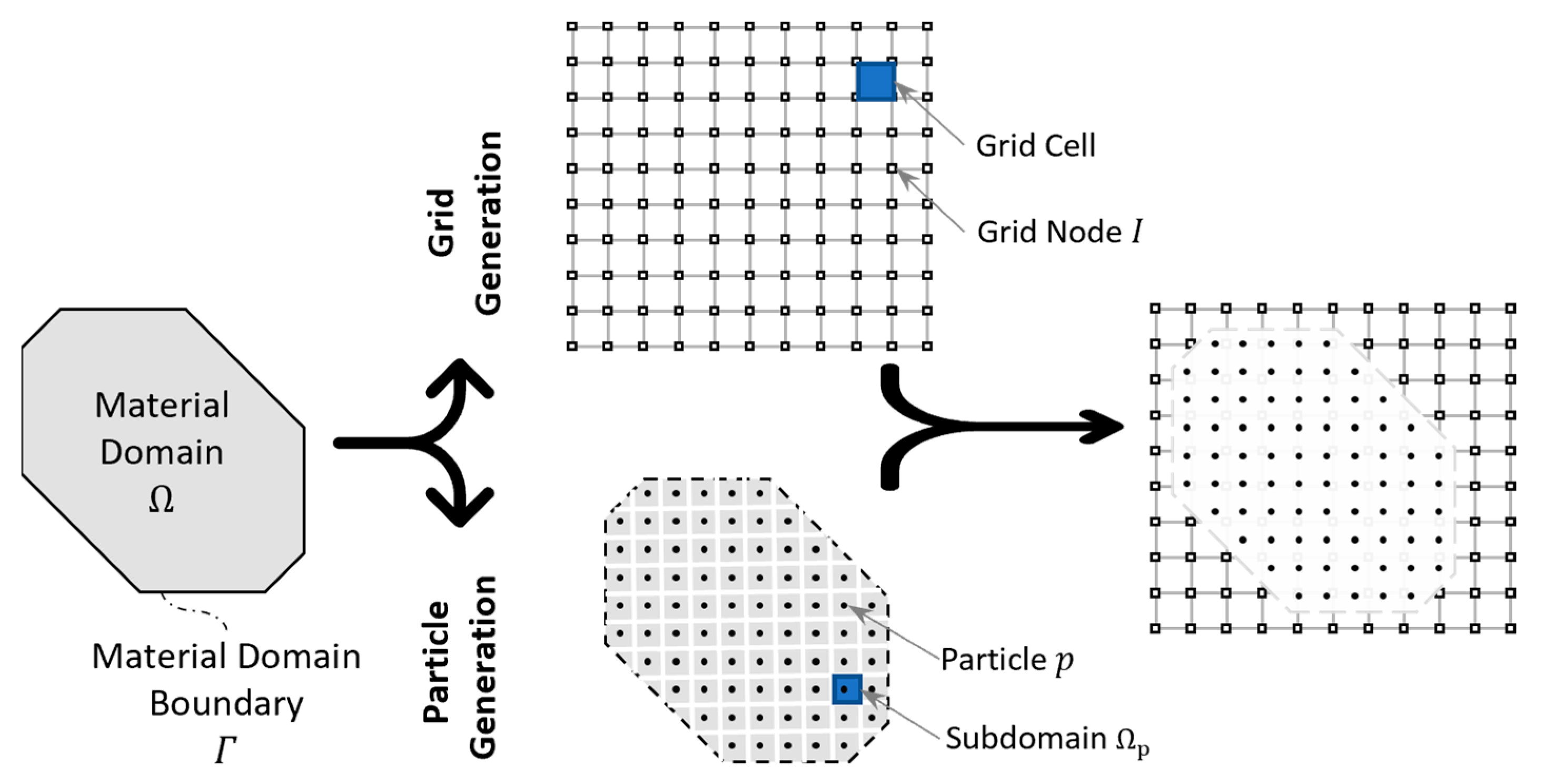
As shown in Figure 1, the continuum material domain $\Omega$ with boundary $\Gamma$ is discretized into a collection of particles. Each particle with an index $p$ stands for a subdomain ${\Omega }_{p,}$ and carries corresponding local physical attributes, such as the mass $m_p$, position $x_p$, velocity $v_p$, acceleration $a_p,$ and so on.

Unlike other mesh-free formulations, such as the SPH or the EFG, the field approximation within the MPM is designed independently of particles, thus avoiding neighbor searching. Instead, a Eulerian background grid is laid, covering all potential particle footprints. The grid consists of $n_n$ nodes with shape functions $S_I$ associated with the node $I$. In this way, any physical field $\Psi$ at any position $x$ can be approximated with:

$$\Psi \left(x\right)={{\displaystyle \sum }}_{I=1}^{n_n}\Psi \left(x_I\right)S_I\left(x\right)$$

(7)

where $\Psi \left(x_I\right)$ denotes the nodal value of the physical field at the node $I$. With Equation (7), displacement, velocity, and acceleration can be estimated as:

$$u\left(x\right)={{\displaystyle \sum }}_{I=1}^{n_n}{u}_I{S}_I\left(x\right),v\left(x\right)={{\displaystyle \sum }}_{I=1}^{n_n}{v}_I{S}_I\left(x\right), \mathrm{and} a\left(x\right)={{\displaystyle \sum }}_{I=1}^{n_n}{a}_I{S}_I\left(x\right)$$

(8)

where the quantities with $I$ as a subscript denote corresponding nodal values.

In the classic MPM, the Galerkin scheme is adopted, where the trial functions ($S_I\left(I=1,\cdots ,n_n\right)$) used for field approximation are also used in composing the test function. In Equation (6), the test function is the virtual velocity $\delta v$, so it can be approximated as:

$$\delta v\left(x\right)={\displaystyle \sum }_{I=1}^{n_n}\delta v_I{S}_I\left(x\right)$$

(9)

where $\delta v_I$ is the virtual nodal velocity at the node $I$.

Substituting the approximations $\mathit{\sigma }\left(x\right)$, $v\left(x\right)$, $a\left(x\right)$, and $\delta v\left(x\right)$ into Equation (6) yields:

$${{\displaystyle \int }}_{{\Omega }_t}\rho \left[{\displaystyle \sum }_{J=1}^{n_n}{a}_J{S}_J\left(x\right)\left]\cdot \right[{\displaystyle \sum }_{I=1}^{n_n}\delta v_I{S}_I\left(x\right)\right]dV+{{\displaystyle \int }}_{{\Omega }_t}\rho {\mathit{\sigma }}^s\left[{\displaystyle \sum }_{I=1}^{n_n}\delta v_I\nabla S_I\left(x\right)\right]dV-{{\displaystyle \int }}_{{\Omega }_t}\rho b\cdot \left[{\displaystyle \sum }_{I=1}^{n_n}\delta v_I{S}_I\left(x\right)\right]dV-{{\displaystyle \int }}_{{\Gamma }_t}\rho {\overline{t}}^s\cdot \left[{\displaystyle \sum }_{I=1}^{n_n}\delta v_I{S}_I\left(x\right)\right]dA=0$$

(10)

Due to the arbitrariness of $\delta v_I$, the following equation must be met for each node $I$ ($I=1,\dots ,n_n$):

$${\displaystyle \sum }_{J=1}^{n_n}{{\displaystyle \int }}_{{\Omega }_t}\rho a_J{S}_J\left(x\right)\cdot S_I\left(x\right)dV+{{\displaystyle \int }}_{{\Omega }_t}\rho {\mathit{\sigma }}^s\nabla S_I\left(x\right)dV-{{\displaystyle \int }}_{{\Omega }_t}\rho b\cdot S_I\left(x\right)dV-{{\displaystyle \int }}_{{\Gamma }_t}\rho {\overline{t}}^s\cdot S_I\left(x\right)dA\equiv 0$$

(11)

which can also be written in compact form:

$${\displaystyle \sum }_{\mathrm{J}=1}^{n_n}{m}_{IJ}{a}_J=f_I^{ext}+f_I^{int}$$

(12)

where $m_{IJ}≔{{\displaystyle \int }}_{{\Omega }_t}\rho \left(x\right)S_I\left(x\right)S_J\left(x\right)dV$ is also called the consistent mass, $f_I^{ext}≔{{\displaystyle \int }}_{{\Omega }_t}\rho \left(x\right)b\left(x\right)S_I\left(x\right)dV+{{\displaystyle \int }}_{{\Gamma }_t}\rho \left(x\right){\overline{t}}^s{S}_I\left(x\right)dA$ is the external nodal force, and $f_I^{int}≔-{{\displaystyle \int }}_{{\Omega }_t}\mathit{\sigma }\left(x\right)\cdot \nabla S_I\left(x\right)dV$ is the internal nodal force.

Since the material properties are only recorded at the particles, the Dirac delta distribution $\delta$ is used to represent the spatial occupation of particles within the classic MPM. In this way, the density field of the total domain can be expressed as:

$$\rho \left(x\right)={\displaystyle \sum }_{p=1}^{n_p}{m}_p\delta \left(x-x_p\right)$$

(13)

where $p$ is the particle index, $n_p$ is the total number of particles, $m_p$ is the particle mass with index $p$, and $x_p$ is the particle position with index $p$. Then, with the identity $\int f\left(x\right)\delta \left(x-x_p\right)=f\left(x_p\right)$, $m_{IJ}$, $f_I^{ext}$, and $f_I^{int}$ are developed into:

$$m_{IJ}={\displaystyle \sum }_{p=1}^{n_p}{m}_p{S}_I\left(x_p\right)S_J\left(x_p\right)$$

(14)

$$f_I^{ext}={\displaystyle \sum }_{p=1}^{n_p}{m}_p{S}_I\left(x_p\right)b\left(x_p\right)+{\displaystyle \sum }_{p=1}^{n_p}\frac{m_p{S}_I\left(x_p\right){\overline{t}}^s\left(x_p\right)}{h}$$

(15)

$$f_I^{int}=-{\displaystyle \sum }_{p=1}^{n_p}{\mathit{\sigma }}_p\nabla S_I\left(x_p\right)V_p$$

(16)

where the boundary layer thickness $h$ is introduced for dimensional consistency.

2.4. A Typical Explicit Workflow

Here is the typical update stress last (USL) formulation for the temporal advancement [7]. For clarity, we use $t$ to denote the current moment and $t+\Delta t$ for the future moment. All physical quantities at the moment $t$ are known, and those at the moment $t+\Delta t$ are to be solved.

First, at the beginning of the time step, particle quantities are mapped to the background grid. In particular, particle mass and momentum are of prior interest, since they lay at the core of motion. Using the partition of unity property of shape functions, ${\displaystyle \sum }_{p=1}^{n_p}{S}_I\left(x\right)=1$, the particle momentum and mass are projected to the grid nodes with the following:

$${\left(mv\right)}_I^t={\displaystyle \sum }_{p=1}^{n_p}{S}_I\left(x_p^t\right){\left(mv\right)}_p^t$$

(17)

$$m_I^t={\displaystyle \sum }_{p=1}^{n_p}{S}_I\left(x_p^t\right)m_p^t$$

(18)

Here, the mass is lumped for computational efficiency, with $m_I={\displaystyle \sum }_{\mathrm{J} =1}^{n_n}{m}_{IJ}$. Then, the nodal velocity is available with $v_I^t=\frac{{\left(mv\right)}_I^t}{m_I^t}$.

Second, the nodal velocities and positions are updated, also conceptually called the ‘advection’. For simplicity, the explicit Symlemetic–Euler time discretization is used like the original MPM, where the position is updated based on the updated velocity.

$$v_I^{t+\Delta t}=v_I^t+a_I^t\Delta t$$

(19)

$$x_I^{t+\Delta t}=x_I^t+v_I^{t+\Delta t}\Delta t$$

(20)

where $a_I^t$ is the nodal acceleration obtained by solving Equation (12).

Third, the updated velocity is projected back to particles in the following way:

$$v_p^{t+\Delta t}={{\displaystyle \sum }}_{I=1}^{n_n}{v}_I^{t+\Delta t}{S}_I\left(x_p^t\right)$$

(21)

$$x_p^{t+\Delta t}={{\displaystyle \sum }}_{I=1}^{n_n}{x}_I^{t+\Delta t}{S}_I\left(x_p^t\right)$$

(22)

With future motion known, the particle stress can be updated. Here, the velocity gradient $L$ is needed and given by:

$$L_p^{t+\Delta t}=\nabla v_p^{t+\Delta t}={{\displaystyle \sum }}_{I=1}^{n_n}{v}_I^{t+\Delta t}\nabla S_I\left(x_p^t\right)$$

(23)

which is requisite for the strain increment $\Delta e_p≔\Delta t·sym\left(L_p^{t+\Delta t}\right)$ and the updated deformation gradient $F_p^{t+\Delta t}=\left(Identity+\Delta t·sym\left(L_p^{t+\Delta t}\right)\right)F_p^t$, where $Identity$ denotes the identity matrix, and $sym\left(·\right)$ denotes the symmetrization operator. For the linear elastic isotropic model, the particle stress can be computed as:

$${\mathit{\sigma }}_p^{t+\Delta t}=\lambda ·I·tr\left(sym\left(F_p^{t+\Delta t}\right)-I\right)+2·\mu ·\left(sym\left(F_p^{t+\Delta t}\right)-I\right)$$

(24)

where $tr\left(·\right)$ is the matrix trace operator; $\lambda$ and $\mu$ are the lame parameters. Of course, constitutive models with more complex behaviors, such as elastoplastic and viscoelasticity, can also be implemented based on ${\mathit{\sigma }}_p^t$, $L_p^{t+\Delta t}$, etc.

Finally, at the end of the time step, the background grid is reset to its original undeformed configuration.

3. Improvement Strategy

In the discretization above, the shape functions of grid nodes and their gradients play vital roles in transferring mass, internal forces, and external forces. In particular, the estimation of internal force involves the first-order derivative.

The piecewise-linear Lagrange basis with $C^0$ continuity obviously cannot provide a smooth derivative, so in the classic MPM, internal nodal forces usually oscillate when particles cross the discontinuity locations. Therefore, the GIMP, the BSMPM, the double domain MPM (DDMPM) [24], and the MLSMPM were successively proposed to provide continuous derivatives. These variants have been proven effective in eliminating numerical noise and promoting stability. However, transfer stencils of the abovementioned MPM variants are enlarged for higher smoothness, especially the currently popular BSMPM. A wider stencil causes higher computational costs of particle-to-grid and grid-to-particle mappings. In particular, the computational cost would be squared or cubed in 2D and 3D cases because of the dyadic product. Even though the accuracy improvement with wide stencil is limited, efficiency has been largely sacrificed.

We found that the hierarchy of Bernstein polynomials has excellent potential, e.g., the partition of unity, to facilitate MPM with more field approximation options. The original Bernstein polynomials are of high continuity, but when they are restricted to a finite element mesh, the continuity at element edges is only $C^0$ and thus not suitable for direct use in the MPM. Therefore, we propose a set of transformations to implement better features. The proposed transformations refer to smoothing and aggregation. For the former, the Bernstein polynomials from the Binomial theory are smoothed with a convolution reformation to eliminate the cell crossing error. For the latter, a node aggregation strategy is implemented to cut down the node demand.

Explicit formulas after transformations are provided in the next section for clarity.

3.1. Basic Requirements of Shape Functions

In some literature, a shape function is also called a weighting or interpolation function, which is used to estimate unknown area based on the range of a discrete set of known data points [25,26]. It is fundamental in numerical computation and analysis. Generally speaking, it should satisfy the following properties [27]:

(1)

The partition of unity (PU), ${{\displaystyle \sum }}_{I=1}^{n_n}{S}_I\left(x\right)=1$ for all $x$.

(2)

The compact support (CS), $S_I\left(x\right)\ne 0$ for locations close enough to node $I$.

(3)

The non-negativity (NN), $S_I\left(x\right)\ge 0$ for all $x$.

Within MPM, the PU property defines completeness and is required for representing rigid motions and constant strains. The CS property can simplify spatial discretization and facilitate efficiency. The NN property ensures positive nodal mass, so that the mass matrix is allowed to be lumped to take the place of consistent mass.

3.2. Bernstein Polynomials

In the binomial theorem [28], a polynomial ${\left(x+y\right)}^n$ is able to be expanded into a sum involving terms of the form $a{x}^b{y}^c$, where the exponents $b$ and $c$ are non-negative integers with $b+c=n$. The coefficient $a$ is known as the binomial coefficient $C_n^b≔\frac{n!}{b!\left(n-b\right)!}$.

When $y$ is taken as $1-x$, the partition of unity constantly forms regardless of the exponent $n$. The related terms are known as the Bernstein polynomials:

$$B_{i,n}\left(x\right)=C_n^i{(x)}^i{(1-x)}^{\left(n-i\right)}$$

(25)

where $0 \le i \le n$. Once the $x$ is restricted among the interval $\left[0,1\right]$, each term is non-negative. In this way, the non-negativity can be completely guaranteed, which is also necessary. Since the interval is finite, compact support is also ensured. Figure 2 shows cubic Bernstein polynomials, which have four components.

The studies of Bernstein polynomials in approximation and solving PDEs can be found in [29,30,31,32,33,34].

3.3. Smooth Transform for Avoiding Cell Crossing Errors

The Bernstein polynomials with the partition of unity can serve as the base for field approximation. For laying Bernstein polynomials, a grid with cells is required to cover the target field. Each cell has edge nodes to connect neighbor cells. Besides edge nodes, there are internal nodes in each cell. The number of internal nodes per cell is relative to the order of polynomials. For instance, in 1D, quadratic Bernstein polynomials require one internal node per cell, and cubic Bernstein polynomials require two internal nodes per cell. Meanwhile, the number of shape functions equals the degree of polynomials, also called the cell order.

Here, the shape function at cell edges is denoted $\mathit{type} \mathrm{I}$, and those at internal cellular nodes are denoted $\mathit{type}\mathrm{II}$, $\mathit{type} \mathrm{III}$, etc. by the position of nodes. The shape functions of $\mathit{type} \mathrm{I}$ have the following form:

$$B_I^{type \mathrm{I}}\left(x\right)=\left\{\begin{array}{cc}\hfill {\left(1-\left|r\right|\right)}^2& for-1\le r\le 1\hfill \\ \hfill 0 & otherwise\hfill \end{array}\right.$$

(26)

where $r=x-x_I$. Those of $type k$ ($2 \le k \le n$, $n$ is the order) have the following form:

$$B_I^{type k}\left(x\right)=\left\{\begin{array}{cc}\hfill C_n^{k-1}{(\xi )}^{k-1}{(1-\xi )}^{\left(n-k+1\right)}& for 0\le \xi \le 1\hfill \\ \hfill 0 & otherwise\hfill \end{array}\right.$$

(27)

where $\xi =x-x_I-\frac{k-1}{n}$. $B$ denotes the original Bernstein shape function.

From Equations (26) and (27), the Bernstein functions are smooth within the cell but still $C^0$ across the cell boundaries. The absence of smoothness at the boundaries makes Bernstein functions unsuitable for the updated Lagrangian MPM.

In this paper, we adopted the following convolving method to enhance the smoothness of the original Bernstein shape functions:

$$S{B}_I^{type k}\left(x\right)=\frac{{{\displaystyle \int }}_{\Re }\chi \left(\zeta -x\right)B_I^{type k}\left(\zeta \right)d\zeta }{{{\displaystyle \int }}_{\Re }\chi \left(\zeta \right)d\zeta }$$

(28)

where $\chi \left(x\right)·\left\{\begin{array}{c}1\\ 0\end{array} \begin{array}{c}\left|x\right|\le 1/2\\ else\end{array}\right.$, and $SB$ denotes a smoothed Bernstein shape function. $\Re$ denotes the whole real domain. Equation (28) improves the level of smoothness by one degree, from $C^0$ to $C^1$. In this way, the smoothed Bernstein shape functions naturally eliminate cell crossing errors [35].

Due to the smoothing effect of convolution, the support domain radius is also enlarged by a half cell. Specifically, in 1D, the shape functions of $type \mathrm{I}$ cover three cells, and the shape functions of other types cover two cells after applying Equation (28). Higher smoothness is available through recursing Equation (28). At the same time, the support domain radius will increase further.

The functions obtained from Equation (28) can be called the smoothed Bernstein shape functions. The smoothed Bernstein shape functions still meet the partition of unity, compact support, and non-negativity. This practically extends the usage of Bernstein functions from the total Lagrangian MPM to the updated Lagrangian MPM.

3.4. Aggregation Transform for Reducing Node Amount

As mentioned above, the Bernstein polynomials require elemental internal nodes. The smoothed ones do as well. Elemental internal nodes may improve field approximation and further numerical precision. However, more nodes are less competitive for efficiency. For example, when using quadratic Bernstein shape functions, each background cell requires 3, 9, and 27 nodes in 1D, 2D, and 3D cases, respectively. In contrast, the quadratic B-spline of $C^1$ smoothness needs only 2, 4, and 8 nodes.

Aimed at efficiency-focused simulation, we propose the following technique to aggregate the shape functions at internal nodes to their nearest neighbor edge nodes.

$$AS{B}_I\left(x\right)=S{B}_I^{Type \mathrm{I}}\left(x\right)+{\displaystyle \sum }_{k=2}^n{a}_k \left[S{B}_{I+k-1}^{type k}\left(x-\frac{k-1}{n}\right)+S{B}_{I-k+1}^{type k}\left(x+\frac{k-1}{n}\right)\right]$$

(29)

where $ASB$ denotes an aggravated and smoothed Bernstein shape function. It should be noted that for any internal node ($k\ge 2$), the superscript $type k$ must consist in the subscript $I+k-1,$ since the formulations of smoothed Bernstein shape functions are highly dependent on the node arrangements. The $a_k$ is a weight parameter related to the relative distance between the node $I+k-1$ and node $I$. We recommend taking $a_k=1$ when $k<\frac{n}{2}$, $a_k=\frac{1}{2}$ when $k=\frac{n}{2}$, and $a_k=0$ when $k>\frac{n}{2}$, so that spatial symmetry can be met.

In essence, Equation (29) approximates the field probes of internal nodes with their nearest neighbor edge nodes. This significantly cuts down the transferring expense between particles and nodes. Specifically, with the aggregation strategy, the quadratic Bernstein shape functions reduce node demand by 1, 5, and 19 in 1D, 2D, and 3D cases, respectively.

Here, we call the shape functions in Equation (29) the aggregated and smoothed Bernstein shape functions. In this way, we obtained a new MPM variant called ASBMPM. It should be noted that the ASB functions meet the partition of unity, compact support, and non-negativity.

4. Formulation Summary

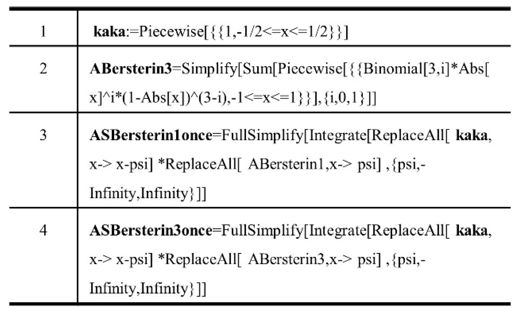
This section provides some of the formulations mentioned above explicitly to make the conceptions easy to implement. However, for simplicity, only several typical ones are listed. For remedy, a piece of Mathematica script (Figure 3) is given as a reference for deriving a higher hierarchy.

There are two independent configuration axes for the ASBMPM scheme, i.e., the selection of the original Bernstein Shape functions and the level of convolving smoothing recursion. To address the hierarchy unambiguously, we use Roman numerals (I, II, III, etc.) to denote the degree of original Bernstein polynomials and ordinal descriptors (quadratic, cubic, quartic, etc.) to indicate continuity level. For example, the ‘quadratic-III ASB’ refers to the subtype developed from three-degree Bernstein Shape functions by aggregating and once smoothing.

Table 1. Formulas of the aggregated-smoothed Bernstein shape functions.

Original Bernstein Degree	Continuity after Aggregation and Smoothing
	Quadratic (after Once Smoothing)	Cubic (after Twice Smoothing)
I	$\left\{\begin{array}{cc}\frac{3}{4}-r^2& 0\le r<\frac{1}{2}\hfill \\ \frac{1}{8}{(3-2r)}^2& \frac{1}{2}\le r<\frac{3}{2}\hfill \\ 0& otherwise\hfill \end{array}\right.$	$\left\{\begin{array}{cc}\frac{1}{6}\left(3\left(r-2\right)r^2+4\right)& 0\le r<1\hfill \\ -\frac{1}{6}{(r-2)}^3& 1\le r<2\hfill \\ 0& otherwise\hfill \end{array}\right.$
II	same as above	same as above
III	$\left\{\begin{array}{cc}{r}^4-\frac{3r^2}{2}+\frac{13}{16}& 0\le r<\frac{1}{2}\hfill \\ -\frac{1}{32}{(2r-3)}^3\left(2r+1\right)& \frac{1}{2}\le r<\frac{3}{2}\hfill \\ 0& otherwise\hfill \end{array}\right.$	$\left\{\begin{array}{cc}\frac{1}{20}\left(-6r^5+15r^4-20r^2+14\right)& 0\le r<1\hfill \\ \frac{1}{20}{(r-2)}^4\left(2r+1\right)& 1\le r<2\hfill \\ 0& otherwise\hfill \end{array}\right.$
IV	same as above	same as above
V	$\left\{\begin{array}{cc}\frac{1}{32}\left(-64r^6+80r^4-60r^2+27\right)& 0\le r<\frac{1}{2}\\ \frac{1}{64}{(3-2r)}^4\left(4r^2+1\right)& \frac{1}{2}\le r<\frac{3}{2}\\ 0& otherwise\end{array}\right.\begin{array}{cc}& \end{array}$	$\begin{array}{cc}\left\{\begin{array}{cc}\frac{3r^7}{7}-\frac{3r^6}{2}+\frac{3r^5}{2}-r^2+\frac{5}{7}& 0\le r<1\\ -\frac{1}{14}{(r-2)}^5\left(r\left(2r-1\right)+1\right)& 1\le r<2\\ 0& otherwise\end{array}\right.& \end{array}$
VI	same as above	same as above
VII	$\begin{array}{cc}\left\{\begin{array}{cc}5r^8-7r^6+\frac{35r^4}{8}-\frac{35r^2}{16}+\frac{221}{256}& 0\le r<\frac{1}{2}\\ -\frac{1}{512}{(2r-3)}^5\left(2r\left(10r\left(2r-1\right)+7\right)+1\right)& \frac{1}{2}\le r<\frac{3}{2}\\ 0& otherwise\end{array}\right.& \end{array}$	$\begin{array}{cc}\left\{\begin{array}{cc}-\frac{5r^9}{6}+\frac{15r^8}{4}-6r^7+\frac{7r^6}{2}-r^2+\frac{13}{18}& 0\le r<1\\ \frac{1}{36}{(r-2)}^6\left(r\left(5r\left(2r-3\right)+12\right)-2\right)& 1\le r<2\\ 0& otherwise\end{array}\right.& \end{array}$
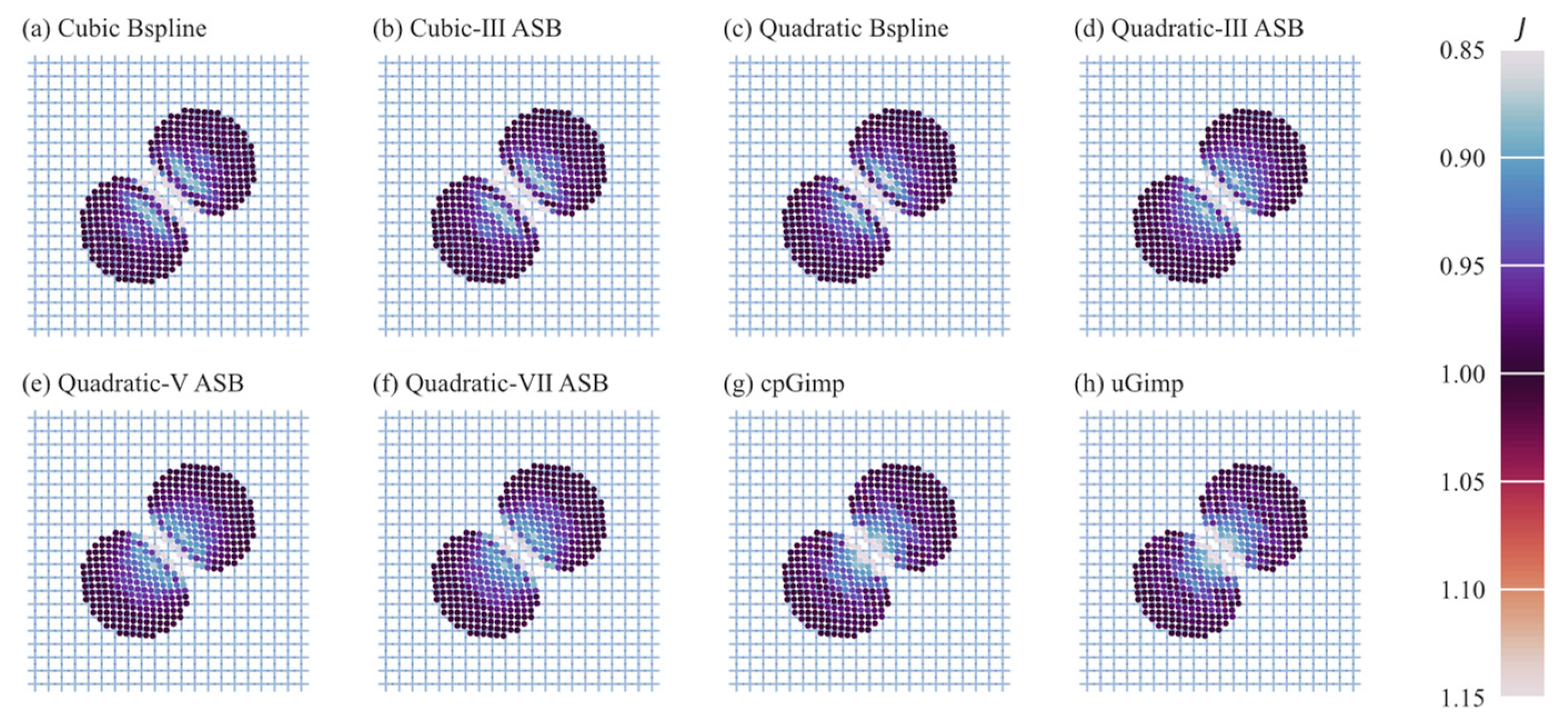
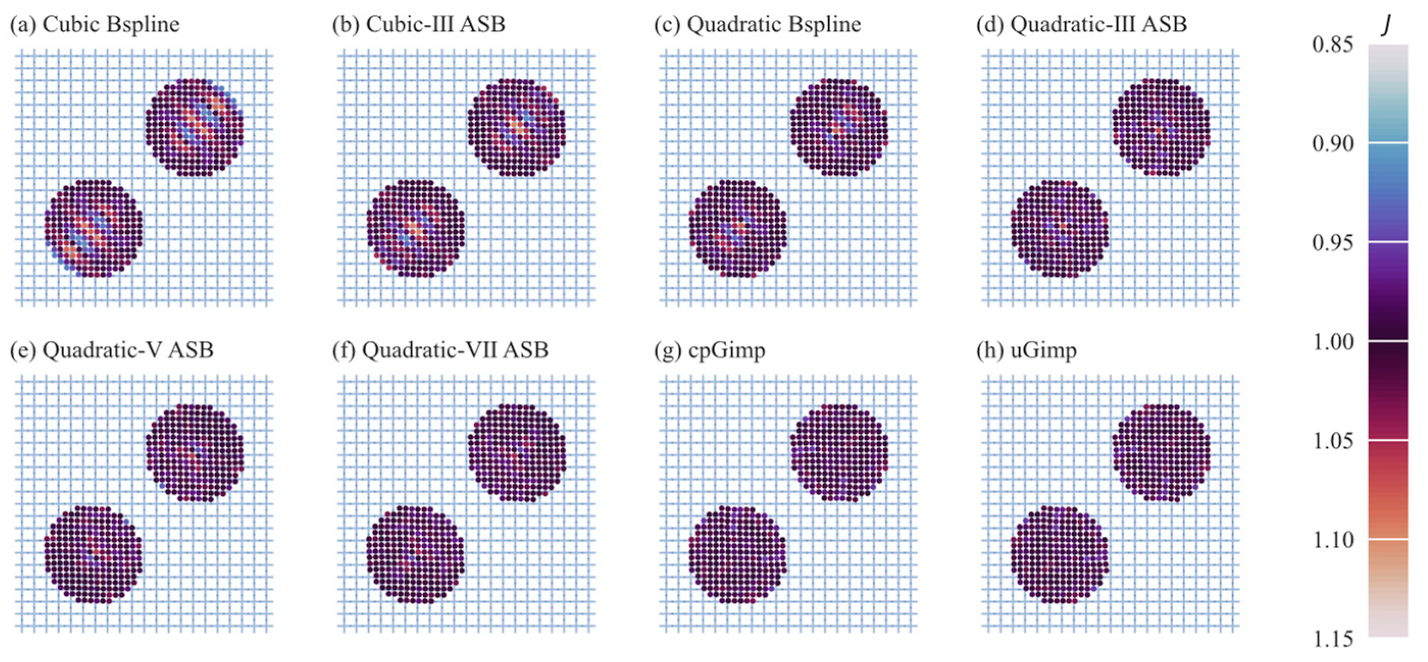
$\mathrm{where} r=\frac{\left|x-x_I\right|}{h}$.

shows the formulas of the quadratic and cubic ASBs of subtypes from I to VII, and they are depicted in Figure 4. In particular, the subtype I is identical to the hierarchy of B-spline shape functions, which can be explained by the convolutive generation of B-spline shape functions [36]. From this point, the relation that the ASBMPM is a superset of BSMPM is self-evident. This implies certain rationality of ASBMPM, since BSMPM has proved to be reliable.

The expressions in Table 1 are univariate. For 2D and 3D problems, the shape functions can be obtained via the tensor-product in all directions, $S_I^{2D}=S_I\left(x\right)S_I\left(y\right)$ and $S_I^{3D}=S_I\left(x\right)S_I\left(y\right)S_I\left(z\right)$, respectively. Due to the multicell dependency, a structured mesh is required in ASBMPM variants.

5. Numerical Validation

Two example problems are considered to demonstrate the performance of the ASBMPM. Both examples are conducted with the Symplicit Euler time integration, and the modified update stress later (MUSL) mode is adopted to avoid the small mass issue [7]. Several popular MPM variants are taken for comparison, including the traditional MPM, BSMPM variants (quadratic, cubic, and quartic), and GIMPs (uGIMP and cpGIMP).

5.1. Axial Vibration of a 1D Continuum Bar

In this section, ASBMPM variants will be examined through a one-dimensional bar vibration problem, which is a classic baseline for validating any MPM variants [27]. In this analytical case (Figure 5), one end of an elastic bar is fixed (at $x=0 \mathrm{m}$), and the other end is free ($x=L=25 \mathrm{m}$, $L$ is the length of the bar). The Young’s modulus of this bar is $E=100 \mathrm{Pa}$, and its density $\rho =1 \mathrm{kg}/{\mathrm{m}}^3$.

Given initial conditions as $u\left(x,0\right)=0$ and $v\left(x,0\right)=v_0\mathit{sin}\left({\beta }_{n}x\right)$, the natural mode $n$ is excited. With the separation of variables [12], the exact position and velocity solutions can be obtained as a reference:

$$u\left(x,t\right)=\frac{v_0}{{\omega }_n}\mathit{sin}\omega t\mathit{sin}{\beta }_{n}x$$

(30)

$$v\left(v,t\right)=v_0\mathit{cos}\omega t\mathit{sin}{\beta }_{n}x$$

(31)

where $v_0$ is the initial velocity amplitude, ${\beta }_n=\frac{2n-1}{2}\frac{\pi }{L}$, and ${\omega }_n={\beta }_n\sqrt{\frac{E}{\rho }}$. For comparison between the continuous analytic solutions and the discrete MPM simulation results, the following mass-weighted solutions are used to benchmark MPM particles:

$$u_{piece}\left(t\right)={{\displaystyle \int }}_{L_{lower}}^{L_{upper}}\rho \left(x\right)u\left(x,t\right)dx/{{\displaystyle \int }}_{L_{lower}}^{L_{upper}}\rho \left(x\right)dx$$

(32)

$$v_{piece}\left(t\right)={{\displaystyle \int }}_{L_{lower}}^{L_{upper}}\rho \left(x\right)v\left(x,t\right)dx/{{\displaystyle \int }}_{L_{lower}}^{L_{upper}}\rho \left(x\right)dx$$

(33)

where $L_{upper}$ and $L_{lower}$ denote the piece range. For a particle $p$ with position $x_p$ and size $l_p$, $L_{upper}=x_p+\frac{l_p}{2},$ and $L_{ower}=x_p-\frac{l_p}{2}$. For the whole bar, $L_{upper}=L$, and $L_{lower}=0$.

In this paper, the vibration mode one is excited ($n=1$), and the timestep meets both the Courant–Friedrichs–Lewy condition ($\frac{v\Delta t}{h}\le 1$) [37] and the dilatational wave speed limit ($\sqrt{\frac{\lambda +2\mu }{\rho }}\le \frac{h}{\Delta t }$), where $h$ denotes the cell size.

5.1.1. Resistance to Cell Crossing Errors

The cell crossing error issue is a gross defect in the MPM variants with the original Bernstein functions [27]. Under a small enough velocity amplitude, the free end particle moves within one single cell so that no cell crossing occurs. However, when the velocity amplitude increases, the free-end particle can cross the cell boundary. We propose the following criteria based on Equation (30) to determine the critical initial velocity amplitude to induce cell crossing events:

$$\frac{v_0}{{\omega }_n}\mathit{sin}\left({\beta }_n\left(L-\frac{1}{2}\frac{h}{n_{ppc}}\right)\right)\ge \frac{1}{2}\frac{h}{n_{ppc}}$$

(34)

where $n_{ppc}$ denotes the number of particles per cell.

In this part, the cell size $h$ is uniformly one unit throughout, and each cell seeds two particles. In this way, the critical initial velocity amplitude is around $0.157 \mathrm{m}/\mathrm{s}$. Therefore, we take $v_0=0.1 \mathrm{m}/\mathrm{s}$ to establish the control group with small displacements and $v_0=0.75 \mathrm{m}/\mathrm{s}$ to induce extreme cell crossing events. The time step size for this simulation is $\Delta t=0.01 \mathrm{s}$ (10% of the Courant–Friedrichs–Lewy limit).

Small Displacement Case ($v_0=0.1 \mathrm{m}/\mathrm{s}$, Duration = 50 s)

Figure 6 gives the vibration results of the particle at the free end under $v_0=0.1 \mathrm{m}/\mathrm{s}$. As the Figure 6a,b shows, the displacement and velocity series are periodic with a period of 10 s all along, which is consistent with the analytical solution. From Figure 6c,d, the relative errors against the analytic solution are also periodic, but amplitudes are gradually increasing. The increasing trend of relative errors is due to the cumulative effect of explicit time stepping. In the case of small displacement, the initial velocity $v_0=0.1 \mathrm{m}/\mathrm{s}$ is too small to induce any cell crossing, so all eleven MPM variants (even the traditional MPM) are below 5% in terms of relative errors. In the ASBMPM hierarchy, variants of higher-degree continuity perform better than those of lower-degree continuity. In particular, the ASBMPM variants score better than the BSMPM variants.

Large Displacement Case ($v_0=0.75 \mathrm{m}/\mathrm{s}$, Duration = 50 s)

According to Equation (34), we increase $v_0$ to displaces particles more and induce cell-crossing events. Under $v_0=0.75 \mathrm{m}/\mathrm{s}$, the traditional MPM is likely to experience the cell crossing error at around 2 $\mathrm{s}$. Figure 7 depicts the vibration results of the particle at the free end. As shown in Figure 7, when using the traditional MPM, the velocity error surges rapidly between 2 s and 2.5 s just at the moment when the particle crosses the cell edge. On the contrary, other MPM variants undergo this period as analytically expected, which convincingly demonstrates the ability of ASBMPM to avoid cell crossing errors. Like the results in the case of small displacement, the ASBMPM variants of higher-degree continuity perform better than those of lower-degree continuity in the ASBMPM hierarchy.

5.1.2. Reduction of Numerical Fracture

The so-called numerical fracture refers to the non-physical separation of edge particles under significant tension. Since particles interact through the background grid in MPM, the numerical fracture issue is related to the support domain size of a shape function. If the support domain radius is small, edge particles can only be attached under slight tension. On the contrary, even large deformations are less likely to result in particle escaping. We propose the following criteria based on Equation (30) to determine the critical initial velocity amplitude to induce numerical fracture events:

$$\frac{v_0}{{\omega }_n}\left[\mathit{sin}\left({\beta }_n\left(L-\frac{1}{2}\frac{h}{n_{ppc}}\right)\right)-\mathit{sin}\left({\beta }_n\left(L-\frac{3}{2}\frac{h}{n_{ppc}}\right)\right)\right]\ge 2R$$

(35)

where $R$ denotes the support domain radius. For piecewise linear, $R=1.0$; for quadratic Bspline and ASB, $R=1.5$; for cubic Bspline and ASB, $R=2.0$.

According to Equation (35), once the critical initial velocity amplitude is increased to $3.0 \mathrm{m}/\mathrm{s}$, no MPM variants can survive numerical fracture events. Therefore, we let $v_0=1.0$, $1.5$, $2.0$, $2.5$, and $3.0 \mathrm{m}/\mathrm{s}$ to study the numerical fracture issue under different shape functions. Figure 8 shows the displacement errors of MPM variants under $v_0=1.0 \mathrm{m}/\mathrm{s}$ and $2.0 \mathrm{m}/\mathrm{s}$. The displacement error series are also periodic.

Figure 9 shows the maximum durations for MPM variants to maintain 1D continuum bar vibration within a 5% error. In the case of $v_0=1.0 \mathrm{m}/\mathrm{s}$, the critical support domain radius is 0.75 times the cell size so that all MPM variants can avoid numerical fracture events. When $v_0$ increases to $2.0 \mathrm{m}/\mathrm{s},$ the critical support domain radius is 1.54 times the cell size, which is just over the support domain radiuses of uGIMP and all quadratic MPM variants, 1.5. Therefore, quadratic MPM variants fail to maintain an error within 5% successively.

The case of $v_0=2.5 \mathrm{m}/\mathrm{s}$ in Figure 9 is able to explain the performance of MPM variants to resist numerical fracture. Specifically, any quadratic ASBMPM variants reach a 5.0% error threshold much later than the quadratic BSMPM, and any cubic ASBMPM variants perform more robustly than the cubic BSMPM. This indicates that ASBMPM variants can perform better than a BSMPM of the same support domain radius as for the numerical fracture issue. Notably, one quadratic ASBMPM variant (Quadratic-V) almost caught up with the accuracy of the cubic BSMPM, even though the support domain of the former is smaller.

5.1.3. Spatial Convergence

The accuracy of the MPM largely depends on spatial and temporal discretization, where the former is improved in this paper. In this section, we estimated spatial errors with the cell size of $1\mathrm{m}$, $2^{-1} \mathrm{m}$, $2^{-2} \mathrm{m}$, $2^{-3} \mathrm{m}$, and $2^{-4} \mathrm{m}.$ To meet the dilatational wave speed limit at any selected cell size, a relatively small timestep, $0.001 \mathrm{s}$, is taken. $v_0$ is set to $0.1 \mathrm{m}/\mathrm{s}$, and other settings remain unchanged.

The following error norm can measure spatial accuracy:

$$e=\underset{0\le t_n\le t_f}{\max }\sqrt{\frac{{{\displaystyle \sum }}_{p=1}^{n_p}{V}_p^{t_n}{\left|u_p\left(t_n\right)-u_a\left(x_p,t_n\right)\right|}^2}{{{\displaystyle \sum }}_{p=1}^{n_p}{V}_p^{t_n}{\left|u_a\left(x_p,t_n\right)\right|}^2}}$$

(36)

where $u_p\left(t_n\right)$ is the numerical displacement at particle $p$, $u_{\mathrm{a}}\left(t_n\right)$ is the exact displacement at particle $p$, $n_p$ is the total number of particles, and $t_f$ is the chosen duration.

The errors from Equation (36) and their corresponding cell sizes are plotted on a log-log scale, and convergence curves for the MPM variants are obtained. Figure 10 confirms that ASBMPM variants (including the BSMPM variants) are of the expected second-order convergence rate when the grid sizing is coarse.

5.2. Impact of Two 2D Elastic Disks

In this section, the ASBMPM variants will be examined through a 2D collision of two elastic disks (Figure 11), initially presented in Sulsky’s first MPM literature [6]. The two 2D elastic disks are under plain strain conditions and move in opposite directions toward each other. They are going to collide and rebound, during which energy conservation can be checked.

The computational domain is a square of side length as $1 \mathrm{m}$, which is discretized into 20 $\times$ 20 uniform cells. Each cell seeds four particles for meshing two disks with radius $r=0.2 \mathrm{m}$. The physical properties of these two disks are: $E=1000 \mathrm{Pa}$, $\upsilon =0.3$, and $\mathsf{\rho }=1000 \mathrm{kg}/{\mathrm{m}}^3$. The time step size taken for this problem is $\Delta t=0.001 \mathrm{s}$ (10% of the Courant–Friedrichs–Lewy limit).

5.2.1. System Energy Conversation

Figure 12 shows energy recovery results under ASBMPM, BSMPM, and GIMP variants. There are three typical stages. Before contact ($t\le 1.25 \mathrm{s}$), all energy is kinetic. During impact $1.25 \mathrm{s}\le t\le 2.50 \mathrm{s}$, kinetic energy slumps to an extremely low level and recovers. The series of strain energy is opposite to that of kinetic energy. The strain energy reaches its maximum value at $t\approx 1.9 \mathrm{s}$, when disk deformation developed the most. After the impact stage, disks leave each other, and a little stress oscillates in the disks. As shown in Figure 12, cubic MPM variants enter the collision stage earlier than quadratic MPM variants but exit later, which is closely related to the support domain size of shape functions.

5.2.2. Contact Feature

Figure 13 depicts deformation distributions at t = 2.0 s. Although no explicit contact law is taken, no-slippery contact is naturally met in all the ASBMPM variants, like the other state-of-art MPM variants. The deformation distributions under the quadratic ASBMPM variants are very close to those of quadratic BSMPM variants, as are the cubic variants. The deformation distribution in the compressed area seems smoother under cubic variants than under quadratic variants, which also relates to the support domain size. Figure 14 gives the deformation results after impact disks. There are heavier oscillations in disks under cubic variants, which is consistent with the results of system energy in Figure 12.

6. Conclusions

In this paper, a scheme of aggregated and smoothed Bernstein functions is proposed to improve the accuracy and efficiency of the material point method (MPM). The newly proposed scheme is composed of three aspects, i.e., Bernstein functions, smoothing, and aggregation. With choices of original Bernstein functions and degrees of smoothing, hierarchical ASBMPM variants are obtained.

In detail, the basic requirements for a proper shape function are reviewed and distilled first. Then, the Bernstein polynomials are smoothed with a convolution reformation to eliminate the cell crossing error. Afterward, an aggregation strategy is implemented to cut down the node amount required for field probing. Among these three aspects, the aggregation strategy is the core contribution of this paper. This design approximates the field probes of internal nodes with their nearest neighbor edge nodes, so it significantly reduces the transfer expense between particles and nodes.

Two classic problems are used to validate typical ASBMPM variants. In the axial vibrations of a 1D continuum bar, ASBMPM variants perform better than BSMPM variants under identical conditions. Notably, one quadratic ASBMPM variant can almost catch up with the accuracy of the cubic BSMPM, even though the support domain of the former is smaller. In the impact of two 2D elastic disks, expected energy evolution is well respected, and reasonable contact features are also observed.

In short, this paper provides a new perspective on function approximation and spatial discretization for the MPM. We believe it is fully compatible with classic MPM frameworks and codes. Implementing ASBMPM variants based on the current MPM libraries requires very few modifications. In addition, since properties such as compact support, the partition of unity, and non-negativity are all well met, the newly proposed shape functions can also be applied to other usages involving function approximation.

References

1. Reed, D.; Bajcsy, R.; Fernandez, M.; Griffiths, J.-M.; Mott, R.; Dongarra, J.; Johnson, C.; Inouye, A.; Miner, W.; Matzke, M.; et al. Computational Science: Ensuring America’s Competitiveness; President’s Information Technology Advisory Committee: Arlington, VA, USA, 2005. [Google Scholar]
2. Gingold, R.A.; Monaghan, J.J. Smoothed Particle Hydrodynamics: Theory and Application to Non-Spherical Stars. Mon. Not. R. Astron. Soc. 1977, 181, 375–389. [Google Scholar] [CrossRef]
3. Nayroles, B.; Touzot, G.; Villon, P. Generalizing the Finite Element Method: Diffuse Approximation and Diffuse Elements. Comput. Mech. 1992, 10, 307–318. [Google Scholar] [CrossRef]
4. Belytschko, T.; Lu, Y.Y.; Gu, L. Element-Free Galerkin Methods. Int. J. Numer. Methods Eng. 1994, 37, 229–256. [Google Scholar] [CrossRef]
5. Liu, W.K.; Jun, S.; Zhang, Y.F. Reproducing kernel particle methods. Int. J. Numer. Methods Fluids 1995, 20, 1081–1106. [Google Scholar] [CrossRef]
6. Sulsky, D.; Chen, Z.; Schreyer, H.L. A Particle Method for History-Dependent Materials. Comput. Methods Appl. Mech. Eng. 1994, 118, 179–196. [Google Scholar] [CrossRef]
7. Sulsky, D.; Zhou, S.-J.; Schreyer, H.L. Application of a Particle-in-Cell Method to Solid Mechanics. Comput. Phys. Commun. 1995, 87, 236–252. [Google Scholar] [CrossRef]
8. Sulsky, D.; Schreyer, H.L. Axisymmetric Form of the Material Point Method with Applications to Upsetting and Taylor Impact Problems. Comput. Methods Appl. Mech. Eng. 1996, 139, 409–429. [Google Scholar] [CrossRef]
9. Harlow, F.H.; Welch, J.E. Numerical Calculation of Time-Dependent Viscous Incompressible Flow of Fluid with Free Surface. Phys. Fluids 1965, 8, 2182. [Google Scholar] [CrossRef]
10. Brackbill, J.U.; Ruppel, H.M. FLIP: A Method for Adaptively Zoned, Particle-in-Cell Calculations of Fluid Flows in Two Dimensions. J. Comput. Phys. 1986, 65, 314–343. [Google Scholar] [CrossRef]
11. Sołowski, W.T.; Berzins, M.; Coombs, W.M.; Guilkey, J.E.; Möller, M.; Tran, Q.A.; Adibaskoro, T.; Seyedan, S.; Tielen, R.; Soga, K. Material Point Method: Overview and Challenges Ahead. In Advances in Applied Mechanics; Elsevier: Amsterdam, The Netherlands, 2021; Volume 54, pp. 113–204. ISBN 978-0-323-88519-5. [Google Scholar]
12. Bardenhagen, S.G. Energy Conservation Error in the Material Point Method for Solid Mechanics. J. Comput. Phys. 2002, 180, 383–403. [Google Scholar] [CrossRef]
13. Bardenhagen, S.G.; Kober, E.M. The Generalized Interpolation Material Point Method. Cmes-Comput. Model. Eng. Sci. 2004, 5, 477–495. [Google Scholar] [CrossRef]
14. Sadeghirad, A.; Brannon, R.M.; Burghardt, J. A Convected Particle Domain Interpolation Technique to Extend Applicability of the Material Point Method for Problems Involving Massive Deformations. Int. J. Numer. Methods Eng. 2011, 86, 1435–1456. [Google Scholar] [CrossRef]
15. Steffen, M.; Kirby, R.M.; Berzins, M. Analysis and Reduction of Quadrature Errors in the Material Point Method (MPM). Int. J. Numer. Methods Eng. 2008, 76, 922–948. [Google Scholar] [CrossRef]
16. Hu, Y.; Fang, Y.; Ge, Z.; Qu, Z.; Zhu, Y.; Pradhana, A.; Jiang, C. A Moving Least Squares Material Point Method with Displacement Discontinuity and Two-Way Rigid Body Coupling. ACM Trans. Graph. 2018, 37, 1–14. [Google Scholar] [CrossRef]
17. Song, J.-U.; Kim, H.-G. An Improved Material Point Method Using Moving Least Square Shape Functions. Comput. Part. Mech. 2020, 8, 751–766. [Google Scholar] [CrossRef]
18. de Koster, P.; Tielen, R.; Wobbes, E.; Möller, M. Extension of B-Spline Material Point Method for Unstructured Triangular Grids Using Powell–Sabin Splines. Comp. Part. Mech. 2021, 8, 273–288. [Google Scholar] [CrossRef]
19. Gao, M.; Tampubolon, A.P.; Jiang, C.; Sifakis, E. An Adaptive Generalized Interpolation Material Point Method for Simulating Elastoplastic Materials. ACM Trans. Graph. 2017, 36, 1–12. [Google Scholar] [CrossRef]
20. Yamaguchi, Y.; Moriguchi, S.; Terada, K. Extended B-spline-based Implicit Material Point Method. Int. J. Numer. Methods Eng. 2021, 122, 1746–1769. [Google Scholar] [CrossRef]
21. Zhang, X. The Material Point Method; Elsevier and Tsinghua University Press Computational Mechanics Series; Elsevier/AP: Amsterdam, The Netherlands; Boston, MA, USA, 2017; ISBN 978-0-12-407716-4. [Google Scholar]
22. An Introduction to Meshfree Methods and Their Programming; Springer: Berlin/Heidelberg, Germany, 2005; ISBN 978-1-4020-3228-8.
23. Katz, V.J. The History of Stokes’ Theorem. Math. Mag. 1979, 52, 146–156. [Google Scholar] [CrossRef]
24. Zhang, D.Z.; Ma, X.; Giguere, P.T. Material Point Method Enhanced by Modified Gradient of Shape Function. J. Comput. Phys. 2011, 230, 6379–6398. [Google Scholar] [CrossRef]
25. Sheppard, W.F.; Chisholm, H. Interpolation. In Encyclopædia Britannica; Cambridge University Press: Cambridge, UK, 1911; Volume 14, pp. 706–710. [Google Scholar]
26. Davis, P.J. Interpolation and Approximation; Courier Corporation: Chelmsford, MA, USA, 1975. [Google Scholar]
27. de Vaucorbeil, A.; Nguyen, V.P.; Sinaie, S.; Wu, J.Y. Material Point Method after 25 Years: Theory, Implementation, and Applications. Adv. Appl. Mech. 2020, 53, 185–398. [Google Scholar]
28. Coolidge, J.L. The Story of the Binomial Theorem. Am. Math. Mon. 1949, 56, 147–157. [Google Scholar] [CrossRef]
29. Hamadneh, T.; Merker, J.; Schimmel, W.; Schuldt, G. Simplicial Bernstein Form and Positivity Certificates for Solutions Obtained in a Stationary Digital Twin by Bernstein Bubnov-Galerkin Method. In Proceedings of the 2022 5th International Conference on Mathematics and Statistics, Paris, France, 17–19 June 2022; ACM: New York, NY, USA, 2022; pp. 41–46. [Google Scholar]
30. Doha, E.H.; Bhrawy, A.H.; Saker, M.A. On the Derivatives of Bernstein Polynomials: An Application for the Solution of High Even-Order Differential Equations. Bound. Value Probl. 2011, 2011, 829543. [Google Scholar] [CrossRef]
31. El-Amrani, M.; El-Kacimi, A.; Khouya, B.; Seaid, M. Bernstein-Bézier Galerkin-Characteristics Finite Element Method for Convection-Diffusion Problems. J. Sci. Comput. 2022, 92, 58. [Google Scholar] [CrossRef]
32. El-Amrani, M.; El Kacimi, A.; Khouya, B.; Seaid, M. A Bernstein–Bézier Lagrange–Galerkin Method for Three-Dimensional Advection-Dominated Problems. Comput. Methods Appl. Mech. Eng. 2023, 403, 115758. [Google Scholar] [CrossRef]
33. Farouki, R.T.; Rajan, V.T. Algorithms for Polynomials in Bernstein Form. Comput. Aided Geom. Des. 1988, 5, 1–26. [Google Scholar] [CrossRef]
34. Lohmann, C.; Kuzmin, D.; Shadid, J.N.; Mabuza, S. Flux-Corrected Transport Algorithms for Continuous Galerkin Methods Based on High Order Bernstein Finite Elements. J. Comput. Phys. 2017, 344, 151–186. [Google Scholar] [CrossRef]
35. Wilson, P.; Wuechner, R.; Fernando, D. Distillation of the Material Point Method Cell Crossing Error Leading to a Novel Quadrature-Based C-0 Remedy. Int. J. Numer. Methods Eng. 2021, 122, 1513–1537. [Google Scholar] [CrossRef]
36. Steffen, M.; Wallstedt, P.C.; Guilkey, J.E.; Kirby, R.M.; Berzins, M. Examination and Analysis of Implementation Choices within the Material Point Method (MPM). Cmes-Comput. Model. Eng. Sci. 2008, 31, 107–127. [Google Scholar]
37. Kubrusly, C.S.; de Moura, C.A.; Lax, L.C. (Eds.) The Courant-Friedrichs-Lewy (CFL) Condition: 80 Years after Its Discovery; Birkhauser/Springer: New York, NY, USA, 2013; ISBN 978-0-8176-8393-1. [Google Scholar]
Figure 1. Schematic diagram of typical MPM discretization.
Mathematics 11 00907 g001
Figure 2. Cubic Bernstein polynomials among a unit interval.
Mathematics 11 00907 g002
Figure 3. Mathematica script demo for deriving aggregated-smoothed Bernstein shape functions.
Mathematics 11 00907 g003
Figure 4. Typical aggregated-smoothed Bernstein shape functions: (a) the quadratic, (b) the cubic. Quadratic B-spline and cubic B-spline are exactly the lowest-level cases of the ASB hierarchy.
Mathematics 11 00907 g004
Figure 5. Problem statement of a 1D continuum bar vibration.
Mathematics 11 00907 g005
Figure 6. D continuum bar vibration results (the free-end particle) for variations of the MPM algorithm under the initial velocity amplitude v 0 = 0.1   m / s : (a) the displacement, (b) the relative error of displacement against the analytic solution, (c) the velocity, and (d) the relative error of velocity against the analytic solution.
Mathematics 11 00907 g006
Figure 7. D continuum bar vibration results (the free-end particle) for variations of the MPM algorithm under the initial velocity amplitude v 0 = 0.75   m / s : (a) the relative error of displacement against the analytic solution, and (b) the relative velocity error against the analytic solution. For clarity, some series are truncated when their relative errors increase beyond 5.0%.
Mathematics 11 00907 g007
Figure 8. D continuum bar vibration (the free-end particle) for variations of the MPM algorithm: (a) the relative error of displacement against the analytic solution under v 0 = 1.0   m / s , (b) the relative error of displacement against the analytic solution under v 0 = 2.0   m / s . For clarity, some series are truncated when their relative error increases beyond 5.0%.
Mathematics 11 00907 g008
Figure 9. Maximum durations for MPM variations to maintain 1D continuum bar vibration within 5% error.
Mathematics 11 00907 g009
Figure 10. Spatial convergence of ASBMPM variants for the problem of 1D axial vibration bar.
Mathematics 11 00907 g010
Figure 11. Problem statement of two 2D elastic disks’ impact.
Mathematics 11 00907 g011
Figure 12. System energy comparison of 2D disks’ collision problem under different MPM shape functions.
Mathematics 11 00907 g012
Figure 13. Impact comparison of 2D disks’ collision problem under different MPM shape functions: (a) cubic B-spline, (b) cubic-Ⅲ ASB, (c) quadratic B-spline, (d) quadratic-Ⅲ ASB, (e) quadratic-Ⅴ ASB, (f) quadratic-Ⅶ ASB, (g) cpGIMP, (h) uGIMP. The moment t = 2.0 s when disks deform the most is chosen. Each particle is colored according to the volume ratio J to reflect deformation distribution.
Mathematics 11 00907 g013
Figure 14. Departure comparison of 2D disks’ collision problem under different MPM shape functions: (a) cubic B-spline, (b) cubic-III ASB, (c) quadratic B-spline, (d) quadratic-III ASB, (e) quadratic-V ASB, (f) quadratic-VII ASB, (g) cpGIMP, (h) uGIMP. The moment t = 3.0 s is chosen. Each particle is colored according to the volume ratio J to reflect deformation distribution.
Mathematics 11 00907 g014