Article

Anisotropy-Based Adaptive Polynomial Chaos Method for Hybrid Uncertainty Quantification and Reliability-Based Design Optimization of Structural-Acoustic System

Key Laboratory of Traffic Safety on Track, Ministry of Education, School of Traffic & Transportation Engineering, Central South University, Changsha 410082, China
*
Author to whom correspondence should be addressed.
Mathematics 2023, 11(4), 836; https://doi.org/10.3390/math11040836
Submission received: 23 December 2022 / Revised: 18 January 2023 / Accepted: 20 January 2023 / Published: 7 February 2023

Abstract

:
The evaluation of objective functions and component reliability in the optimisation of structural-acoustic systems with random and interval variables is computationally expensive, especially when strong nonlinearity exhibits between the response and input variables. To reduce the computational cost and improve the computational efficiency, a novel anisotropy-based adaptive polynomial chaos (ABAPC) expansion method was developed in this study. In ABAPC, the anisotropy-based polynomial chaos expansion, namely the retained order of polynomial chaos expansion (PCE) differs from each variable, is used to construct the initial surrogate model instead of first-order polynomial chaos expansion in conventional methods. Then, an anisotropy-based adaptive basis growth strategy was developed to reduce the estimation of the coefficients of the polynomial chaos expansion method and increase its computational efficiency. Finally, to solve problems with probabilistic and interval parameters, an adaptive basis truncation strategy was introduced and implemented. Using the ABAPC method, the computational cost of reliability-based design optimisation for structural-acoustic systems can be efficiently reduced. The effectiveness of the proposed method were demonstrated by solving two numerical examples and optimisation problems of a structural-acoustic system.

1. Introduction

Reliability-based design optimisation (RBDO) has attracted increasing attention in the field of structural-acoustic reliability. Structural-acoustic systems refer to complex systems comprising structures, coupled interfaces, and acoustic cavities [1]. In engineering practice, unavoidable uncertainties, such as initial conditions, external excitation, material characteristics, boundary conditions, and external environment, exist [2]. Accordingly, the RBDO of structural-acoustic systems with uncertain parameters has recently garnered extensive attention.
Reliability optimisation requires an appropriate uncertain model to quantify the uncertainty parameters. Recently, reliability optimisation models for structural-acoustic systems have been built to handle uncertain information, including probability models, interval models, and hybrid probabilistic and interval models. In the case of probability models, the uncertainty should be represented by a precise probability distribution of an uncertain parameter made available from many samples. In the case of interval models, it is not necessary to obtain the exact distribution function; instead, it is sufficient to represent the uncertainty of an uncertain parameter by its upper and lower bounds [3]. In engineering practice, both uncertain models that mentioned above are common. This study mainly investigates reliability analysis and optimisation problems under hybrid probabilistic and interval models.
RBDO with hybrid probabilistic and interval parameters is comparatively complex and can be considered a three-loop optimisation problem. The inner and middle loops help evaluate the objective function and limit state function, respectively, and analyse their probabilistic statistics in extreme cases. The computational burden in each iteration is considerable due to the large number of uncertainty analyses of the inner and middle loops [4]. Two common methods have been employed to increase the computational efficiency of RBDO with probabilistic and interval variables. One of them is decoupling, which converts a nested optimisation problem into a single-loop optimisation problem. Du et al. [5] made an early attempt to convert a hybrid RBDO problem of the inner loop into a single-loop optimisation problem. This method was further extended to a hybrid RBDO problem with dependent interval variables [6]. Subsequently, Kang and Luo et al. [7,8] developed a valid single-loop decoupling method based on linearisation and optimality conditions for performance functions. Torii and Lopez et al. [9] proposed a decoupling sum method that can be applied to different reliability analysis methods based on the sequence optimisation and reliability evaluation method. Wang C et al. [10] proposed a novel reliability-based optimization method for thermal structure with hybrid random, interval, and fuzzy parameters.
The computational burden in uncertain optimisation can also be reduced by increasing the computational efficiency of probabilistic interval analyses. The efficiency problem in an uncertain analysis with probabilistic and interval variables is typically solved using the perturbation method and polynomial chaos expansion (PCE) method. Xia et al. [1] utilised an uncertain analysis method based on the perturbation method to solve the objective function and reliability constraint, effectively reducing the computational burden in the RBDO of structural-acoustic systems. Although the perturbation method is computationally efficient, it has limitations in the case of structural-acoustic problems with less uncertainty [11]. Generally, the polynomial expansion method can be divided into the Kriging model expansion, gPC expansion, Chebyshev expansion, and arbitrary PCE methods. Yang and Liu et al. [12] proposed a combined Monte Carlo simulation (RS-MCS) method, and a novel optimisation method for Karush–Kuhn–Tucker conditions was proposed to increase the efficiency of the reliability analysis. Wu et al. [13,14] used the gPC expansion and Chebyshev expansion methods to construct a polynomial basis with probabilistic and interval parameters, respectively, and calculated the response of a hybrid uncertain structural-acoustic system. However, because of the limitations of the gPC expansion method itself, a hybrid uncertain problem with an arbitrary probability density function (PDF) cannot be solved. Yin et al. [15] integrated the aPC expansion with the Chebyshev expansion method to improve the computational accuracy when solving a hybrid uncertainty problem with arbitrary PDFs. Hamdia K M et al. [16] operate the application of PCEs in sensitivity analysis for the mechanics of tendons and ligaments. Compared with the perturbation method and other surrogate model methods, the arbitrary PCE method has the following advantages. First, the statistical characteristics of a system’s response can be acquired using its expansion coefficient, avoiding complex probability integration; second, surrogate models with different fidelity requirements can be established through polynomial optimisation.
The calculation efficiency in solving uncertain engineering problems using the arbitrary PCE method mainly depends on the solution efficiency of the expansion coefficient. The original approach to solving the expansion coefficient involves applying the total-order expansion method, in which the polynomial expansion orders are identical for different variables. The novel Legendre polynomial expansion method developed by Wang et al. [17] utilises the full-order expansion method and Latin hypercube sampling to compute the expansion coefficients. However, this approach has a comparatively higher computational cost than the Taylor-based approach. A sequential sampling strategy has been developed to increase the efficiency of PCE sampling. Wu et al. [13] used the total-order expansion method and sequential sampling to propose a novel high-order polynomial surrogate model, which would be unstable if other sampling methods were used instead of the Chebyshev sampling method. Zhu et al. [18] used the total-order expansion method and sparse-grid sequential sampling to develop a novel sparse-polynomial expansion method. The computational efficiency was significantly improved without compromising the precision using this method. However, none of these methods are suitable for cases where the number of variables is extremely large, and the expansion orders vary significantly for different variables. In a structural-acoustic system, the sensitivity of the system response to different parameters varies significantly. For a structural-acoustic problem, Yin et al. [19] adopted a tensor-product method to calculate the expansion coefficients; this method can retain different polynomial expansion orders for different variables. However, with an increase in the number of input parameters, the computational cost quickly increases, making it unsuitable for multivariate cases. To further reduce the computational cost, Thapa et al. [20] proposed a novel method to obtain stochastic models of responses based on an adaptive algorithm. This method firstly constructs the initial surrogate model N 0 by first-order expansion, then constructs the high-order surrogate model N 1 by adaptive convergence criterion. The advantages of the adaptive PCE include the following: (1) The surrogate model of the adaptive PCE method is simple and convenient for optimization; (2) less sampling points are required to construct the surrogate model, which means higher computational efficiency can be obtained. Meanwhile, owing to its substantial computational savings, the adaptive PCE has been widely implemented in many applications, such as nonlinear random vibration analysis [21], nonintrusive projection [21,22,23,24,25], stochastic finite element analysis [26,27], and benchmark problems [20].
Clearly, many uncertainty analysis algorithms have been proposed to increase the calculation efficiency of uncertain optimisation [28,29], particularly the adaptive PCE method, which has a high calculation accuracy and efficiency. However, when constructing a surrogate model for a system with high-dimension variables and strong nonlinearity, the conventional adaptive PCE will be also inefficient. The main reason is that lots of polynomial update iterations are required from the construction of initial surrogate model N 0 to the final high-order surrogate model N 1 , while the computational burden of each iteration is relatively large for uncertainty problem with high-dimension variables. It should be noted that strong nonlinearity usually exhibits between the system response of the actual structural-acoustic problem and part of variables. Therefore, it is eagerly to develop a method for uncertainty analysis and reliability-based optimization for structural-acoustic problems.
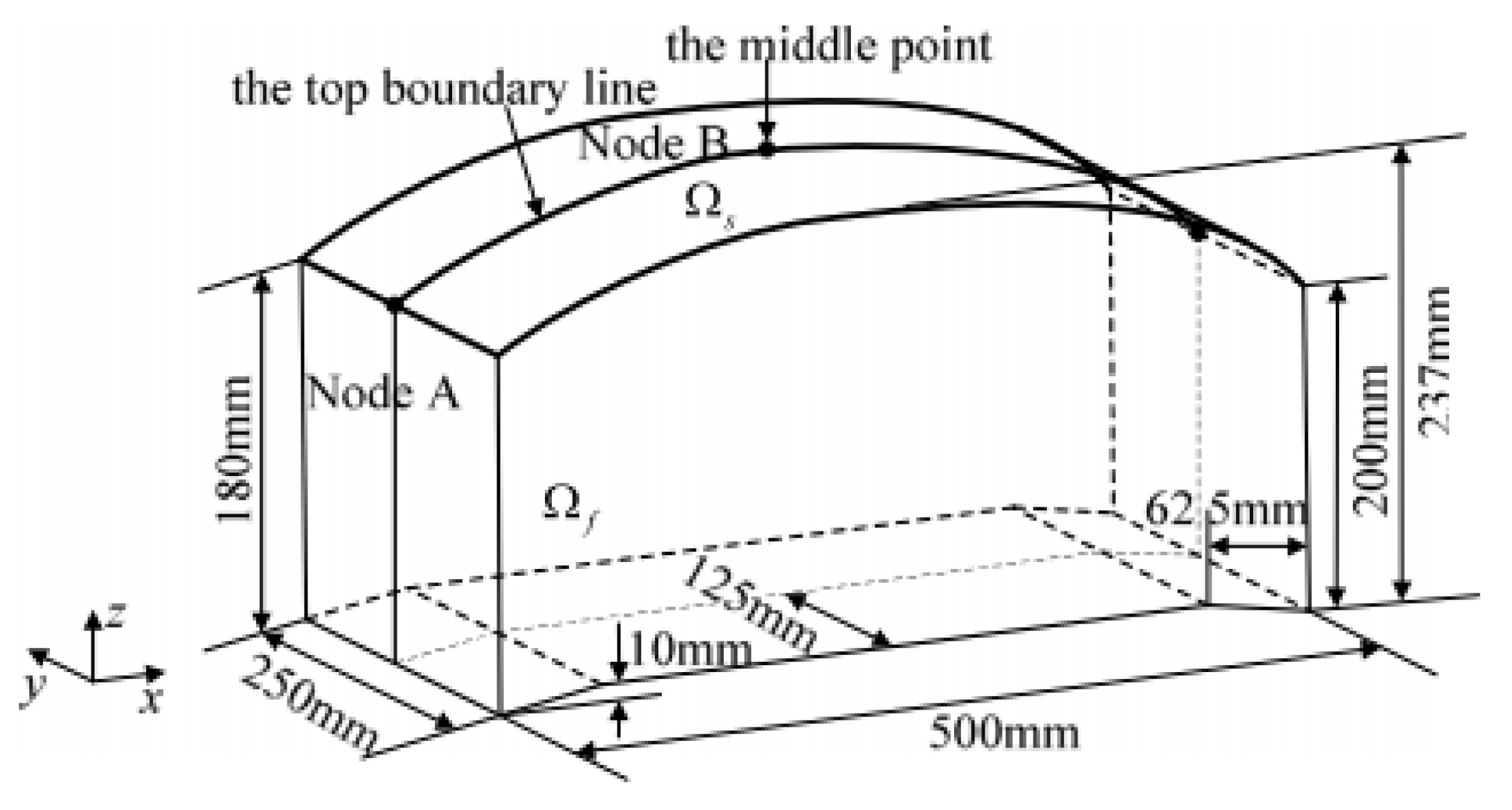
In this paper, a novel anisotropy-based adaptive PCE method, called ABAPC, was developed to address the computational cost and accuracy problems in the reliability optimisation of structural-acoustic systems. Based on this method, hybrid uncertainty quantification and RBDO were performed on a structural-acoustic system. First, an adaptive PCE was suggested to reduce unnecessary computations in the polynomial expansion mode. Subsequently, an anisotropy-based initial surrogate model was proposed to handle the anisotropy of structural-acoustic systems and further reduce the computational burden. Thus, to decrease the number of polynomial basis terms and effectively increase the computational efficiency in the reliability optimisation of structural-acoustic systems, a novel adaptive algorithm was implemented.
The remainder of this paper is organised as follows. In Section 2, a moment-based arbitrary polynomial chaos (MAPC) approach for hybrid uncertainty quantification is described. In Section 3, we propose an anisotropy-based adaptive PCE method, and in Section 4, we discuss the application of this method to the RBDO of a structural-acoustic system. In Section 5, the efficiency and effectiveness of the ABAPC are demonstrated by solving two numerical examples and optimisation problems of a structural-acoustic system. Finally, the conclusions are presented in Section 6.

2. Moment-Based Arbitrary Polynomial Chaos Expansion for Hybrid Uncertainty Quantification

2.1. MAPC Approximation

The PCE can be understood as a process of approximating the uncertainty by utilising the sum of the orthogonal polynomials with independent variables [30]. The PCE for approximating a function can be expressed as follows:
F ( x ) = i = 0 N f i φ i ( x )
where the retained order of an arbitrary PCE is represented by N, and φ i ( x ) represents the polynomial basis of order I, which is different for random variables with different PDFs. The term f i is the expansion coefficient of an arbitrary PCE that must be estimated.
The orthogonal polynomial of the MAPC approximation obtained by the recurrence relationship is expressed as follows:
b j φ j ( x ) = ( x a j ) φ j 1 ( x ) + b j 1 φ j 2 ( x )
where a j and b j denote recurrence coefficients. A more detailed derivation can be found in [31].
According to the Gaussian integration formula, the expansion coefficient f i in Equation (1) can be expressed as follows:
f i = 1 h i R F ( x ) φ i ( x ) ω ( x ) d x = 1 h i i = 1 m F ( x ^ ) φ i ( x ^ ) ω i
where x ^ represents the Gauss integration nodes, and m denotes the total number. ω i represents the Gaussian integration weights. Additionally, there is h i = φ i 2 x , where x ^ and ω i can be calculated using the eigenvalue decomposition of the Jacobi matrix J n , which is expressed as follows:
J n = a 0 b 1 b 1 a 1 b 2 b 2 a n 2 b n 1 b n 1 a n 1
The eigenvalue decomposition of J n can be expressed as follows:
Q T J n Q = d i a g ( λ 1 , λ 2 , , λ n ) Q T Q = I
where I denotes the n × n dimensional identity matrix. Therefore, the nodes and weights can be expressed as follows:
x i = λ i , ω i = b 0 q i , 1 2 , i = 1 , 2 ,
where q i , 1 denotes the first element of the ith column vector in Q . The interval variable is treated as a random variable evenly distributed over the interval, and its expansion coefficient and polynomial basis can be obtained by referring to Equations (1)–(6).

2.2. Moment-Based Arbitrary Polynomial Chaos Expansion for Hybrid Analysis

For multi-dimensional uncertain problems, F ( x ) with interval and random variables can be approximated as follows:
F = F ( x I , x R ) = i 1 = 0 N 1 i L = 0 N L f i 1 , , i L φ i 1 , , i L 1 x I φ i L 1 + 1 , , i L 2 x R
where x = [ x R , x I ] represents all the uncertain variables, x j R ( j = 1 , 2 , , L 1 ) denotes the j-th random variable, and x j I ( j = 1 , 2 , , L 2 ) is the j-th interval variable. L 1 and L 2 denote the numbers of random and interval variables, respectively. The retained order of the MAPC expansion is denoted by N j ( j = 1 , 2 , , L ) , where f i 1 , , i L represents the expansion coefficient, and φ i 1 , , i L ( x ) denotes the L-dimension polynomial basis, which is defined as follows:
φ i 1 , , i L 1 ( x R ) = k = 1 L 1 φ i k ( x k R ) ;   φ i L 1 + 1 , , i L ( x I ) = k = L 1 + 1 L φ i k ( x k I )
where the i k -order polynomial basis for random variables φ i k ( x k R ) can be calculated using the moment of the random variables. φ i k ( x k I ) represents the i k -order polynomial basis with an interval variable, which is orthogonal to the weight function of the Chebyshev polynomial. According to the above equation, as the number of variables increases, the computational cost of constructing a polynomial basis increases exponentially.
By using the Gauss integration, f i 1 , , i L can be obtained and expressed as follows:
f i 1 , , i L = 1 h 1 × × h L R R F ( x ) φ i 1 , , i L ( x ) ω i 1 , , i L ( x ) d x = 1 h 1 × × h L j 1 = 1 M 1 j L = 1 M L Y ( x ^ I , x ^ R ) φ i 1 , , i L 1 ( x ^ I ) φ i L 1 + 1 , , i L ( x ^ R ) ω i 1 , , i L
where x ^ I and x ^ R represent the Gauss integration nodes for x R and x I , respectively. M k ( k = 1 , 2 , , L ) represents the total number of integration nodes with respect to x k .
The total number of integration points to estimate f i 1 , , i L can be determined by the following:
N tot = ( N 1 + 1 ) × ( N 2 + 1 ) × × ( N L + 1 )
From the above formula, we find that N tot and f i 1 , , i L increase exponentially with the increase in the retained order and number of variables. Thus, the computation of the coefficients of an arbitrary PCE using the Gauss integration technique for high-order and multi-dimensional problems is extremely cumbersome and time-consuming. A simplex format was introduced into the arbitrary PCE to increase the efficiency and precision of high-order orthogonal PCE for multi-dimensional problems. Equation (7) can be rewritten as follows:
F = F ( x I , x R ) = 0 i 1 + + i L 1 + + i L n f i 1 , , i L φ i 1 , , i L 1 x I φ i L 1 + 1 , , i L x R ,   i 1 , , i L = 0 , 1 , , n .
Thus, the number of expansion coefficients is reduced to the following:
N c ( n , L ) = ( n + L ) ! L ! n !
The least-squares method (LSM) can be used to calculate the coefficients of the polynomials. Thus, Equation (11) can be rewritten as follows:
F ( x ) = β T α
β = [ β 1 β s ] T = [ f 0 0 , , f i 1 i L ] T , 0 i 1 + + i L n
α = [ α 1 α s ] T = [ φ 0 0 , , φ i 1 i L ] T
where α represents a polynomial basis vector, β represents a coefficient vector, s denotes the number of expansion coefficients, and s = N c . β is obtained by LSA, which can be expressed as in Equation (16):
β = A T A 1 A T Y
Y = [ F ( x 1 I , x 1 R ) F ( x s I , x s R ) ] , s = N C
A = α 1 ( x 1 I , x 1 R ) α s ( x 1 I , x 1 R ) α 1 ( x s I , x s R ) α s ( x s I , x s R ) , s = N C
where α 1 ( x 1 I , x 1 R ) , , α s ( x s I , x s R ) denotes all the sampling points.
Therefore, it is apparent that the precision and efficiency of the PCE method based on the sequential sampling scheme are significantly influenced by the sampling schemes. Conventionally, Latin hypercube sampling [32] has been easily implemented; however, it has drawbacks, such as lack of flexibility and instability. To increase the efficiency and stability of PCE sampling, a sequential sampling strategy was developed. However, the number of candidates increases exponentially. Compared with the previous scheme, the square grid sampling scheme can help improve the computational efficiency. However, its accuracy is not as stable as that of the former. Therefore, the sequential adaptive sampling strategy is introduced in the next section.

3. Anisotropy-Based Adaptive Polynomial Chaos Expansion Method

The response of an uncertain structural-acoustic system exhibits anisotropy, and the complexity of each dimension varies significantly. Existing expansion methods are inefficient in solving multi-dimensional and strongly anisotropic problems. Moreover, an excessive number of polynomial basis terms can increase the computational burden of optimisation when using a surrogate model. To solve the above problems, the proposed method employs the following steps. First, the anisotropy-based polynomial chaos expansion is used to construct the initial surrogate model in high-order and multi-dimensional problems. Second, an anisotropy-based adaptive basis growth strategy is proposed based on the adaptive strategy to reduce the estimation for the coefficients of the PCE method and improve the computational efficiency of the PCE method. Finally, an adaptive basis truncation strategy based on the contribution of the variance was introduced and implemented to solve problems with probabilistic and interval parameters. The specific steps of the ABAPC method proposed in this section are as follows.

3.1. Anisotropy-Based Initial Surrogate Model

Treating each dimension isotropically means that each dimension is treated in the same manner. However, this assumption only applies to problems in which there is little difference in the complexity of each dimension. In other words, if the problem exhibits significant differences between dimensions, the method requires a large number of polynomial update iterations to converge. Thus, it is desirable to consider the anisotropy in the PCE-based adaptive basis truncation strategy [33,34]. Therefore, an anisotropy-based initial surrogate model was proposed in this section to address this problem.
The anisotropy-based initial surrogate model can be built by obtaining an initial expansion-order vector that considers the complexity of each dimension, which can be defined as follows:
N 0 = { n 1 0 , n 2 0 , , n l 0 }
where the initial expansion order of the rth variable in the anisotropy-based initial surrogate model is defined as n r 0 ( r = 1 , , l ) , and N 0 denotes the l-dimensional initial expansion order vector. Therefore, based on the idea that transforms a multi-dimensional problem into a one-dimensional problem, the main steps for obtaining the initial expansion order of each dimension in the PCE method are as follows:
Step 1: Input dimension r of the PCE and treat the other dimensions as constants;
Step 2: Obtain the response of the PCE by the method described in Section 2.2.;
Step 3: Calculate the relative errors in the expectation and variance by Equations (20) and (21);
Step 4: If the maximum value of the errors is less than the given tolerance e r t o l , stop
Otherwise, the order n r 0 is increased to n r 0 + 1 , and Steps 3 and 4 are repeated until the error is satisfied;
Step 5: Steps 1–4 are repeated until all the initial expansion orders for l dimensions are obtained. Output the initial expansion-order vector N 0 = { n 1 0 , n 2 0 , , n l 0 } .
Here, the relative errors in the expectation and variance can be determined as follows:
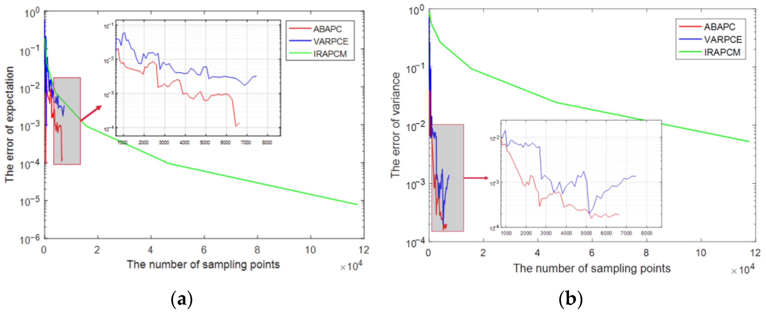
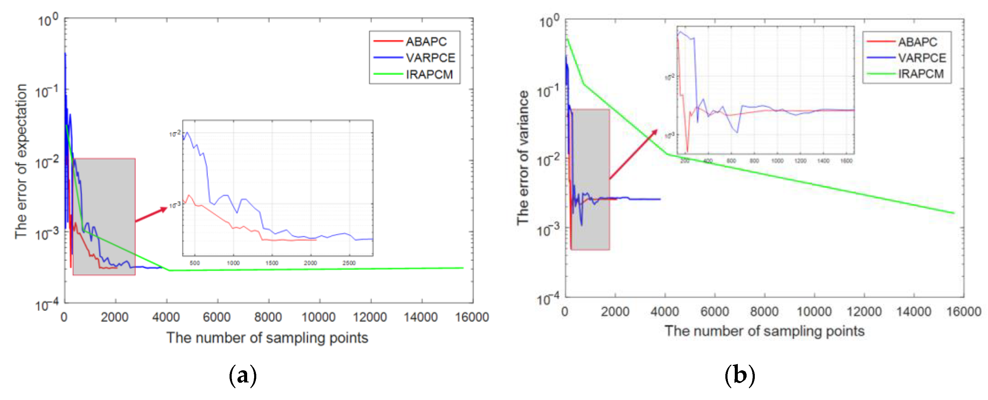
e r σ = σ 2 σ 2 r e f σ 2 r e f
e r μ = μ μ r e f μ r e f
In Equations (20) and (21), σ r e f 2 and μ r e f represent the reference results obtained using the Monte Carlo method (MCM). The number of sampling points for the random (interval) variables of the MCM was set to 10,000. The number of sampling points for obtaining σ is determined by the expansion order. The precision of the PCE method was obtained by iteratively increasing the order of the PCE until the maximum value of e r σ and e r μ is less than the given tolerance e r t o l , which was set as 10−2 in this study. Further applications of the anisotropy-based initial surrogate model are presented in the next section.

3.2. Anisotropy-Based Adaptive Basis Growth

The adaptive enrichment of the polynomial basis proposed in [20] treats each dimension isotropically, leading to unnecessary computations for problems with strong anisotropy. To reduce the estimation of the coefficients of the PCE method and increase its efficiency, a weight vector based on the anisotropy-based initial surrogate model was proposed. A new basis set was obtained by adaptively adding a new polynomial basis based on the weight vector.
Iteratively increasing the order of the PCE is the conventional method for enhancing the precision of the PCE approach with a given number of samples. Therefore, a PCE model with order N p + 1 can be constructed based on existing available information of the PCE method with the order N p . Subsequently, the number of additional polynomial basis terms added can be represented by N u m . ( φ i n c r e a s e ) and is expressed in Equation (22).
N u m . ( φ i n c r e a s e ) = N u m . ( φ N p + 1 n ) N u m . ( φ N p n )
Here, Num.() represents the cardinality of the set. N u m . ( φ i n c r e a s e )  increases exponentially with increasing retained order of the PCE, which significantly increases the computational amount for obtaining the response of an uncertain structural-acoustic system/(multi-dimensional problems). To mitigate this effect, a polynomial basis can be selected a priori by implementing specific strategies. However, because the rank and sparsity of solutions are typically not known in advance, the importance of the polynomial basis cannot be realized in advance. Therefore, an adaptive enrichment basis polynomial is required to extract the maximum amount of information from a given number of samples.
The adaptive enrichment of the old basis set of order N p is achieved by adaptively adding a new polynomial basis in blocks to obtain new basis sets of order N p + 1 , instead of adding all the polynomials of φ i n c r e a s e . The number of polynomial basis terms in each block R n is given by Equation (19). Each chunk is assigned an equal number of polynomial basis terms. However, the last one contains leftover basis polynomials if this requirement cannot be satisfied. The total number of chunks of φ i n c r e a s e represented by R s is given by Equation (24).
R n = log ( n ) × N u m . ( φ i n c r e a s e )
R s = N u m . ( φ i n c r e a s e ) R n
Here, ⌈ ⌉ represents the real part of the number. The basis set of the early adaptive selection algorithm, proposed by A at al. [20], was gradually enriched by adding R n new polynomials at a time. In this study, the basis set of the PCE method was updated by adding a group of polynomial basis φ a d d A S M A P C to the old basis set φ o l d A S M A P C , obtaining a new set φ n e w A S M A P C , which is expressed as follows:
φ n e w A S M A P C = φ o l d A S M A P C φ a d d A S M A P C
In the adaptive enrichment of a polynomial basis based on the adaptive basis truncation strategy, each dimension is treated isotropically. The expansion order of each variable in each iteration is increased by one level. To consider the anisotropy in the operation of adaptive enrichment, ω = ω 1 , ω 2 , , ω m can be defined as an l-dimensional weight vector for each variable. The anisotropy-based adaptive enrichment of the existing basis set, which includes a polynomial basis with the initial expansion order N 0 , is to obtain new basis set with an updated order N by adaptively adding a new polynomial basis based on ω = ω 1 , ω 2 , , ω l . After anisotropy-based adaptive enrichment of the existing expansion-order vector, the updated expansion-order vector is defined as follows:
N = N 0 + m × 1 ω ¯ × ω m = 1 , , N max
ω r = n r 0 r = 1 l n r 0 , r = 1 , 2 , , l
where N denotes the updated l-dimensional expansion-order vector. The term m represents the expansion order to be increased for each variable, ω ¯ = max 1 r l   ω r   [   ] represents the integral part of the value in Equation (26), and the weight vector ω can be obtained from Equation (27).
As mentioned above, the anisotropic method can account for problems in which each dimension is not equally important by appropriately setting the weight vector. This can be explained by the fact that, the higher the weight value in the anisotropic formula, the higher the importance. For example, the isotropic adaptive basis truncation strategy is a special case for the anisotropic method. The initial expansion orders of each dimension and components of the weight vectors are equal. This implies ω 1 = ω 2 = = ω l . In other words, the anisotropic method can be treated as a more generalised version of the isotropic adaptive-basis truncation strategy.
For instance, a four-dimensional problem is considered as in Equation (28):
f ( x ) = e x 1 + x 1 4 + x 2 × x 3 + x 4
where x y ( y = 1 , 2 , , 4 ) represents the independent uncertain parameters, which can be assumed as a linear function of the random variable. 
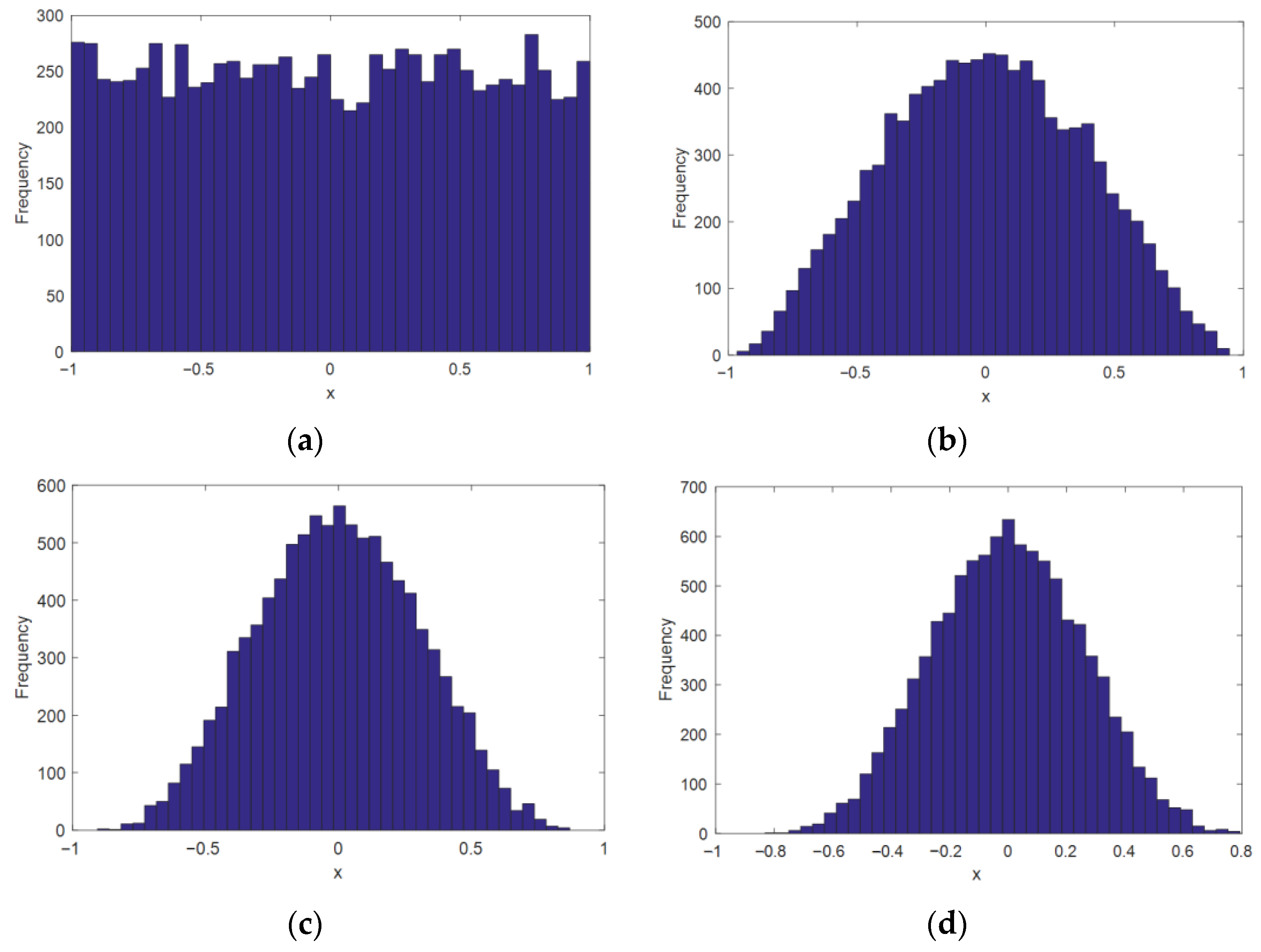
Table 1 presents the uncertainty information and deformed function of each uncertain parameter. In this case, each random variable is uniformly distributed in the range [−1, 1].
From Table 1, the order vector of the initial expansion order can be set to N 0 = { 3 , 1 , 1 , 1 } . The weight vector ω = { 50 % , 16.7 % , 16.7 % , 16.7 % } can be calculated using Equation (23). Table 2 presents the order vectors of the proposed approach and the isotropic adaptive polynomial chaos expansion (IAPCE) approach updated as an increase in m. The number of sampling points can be set as 1.5 times the number of basis terms before the basis truncation operation.
As shown in Table 2, the sampling points in the ABAPC method are fewer than those in the IAPCE method. The advantages of the proposed method become increasingly evident with increasing number of variables.
Traditional arbitrary PCE method requires extensive calculation of the expansion coefficients. However, the adaptive expansion method can require a smaller number of estimates for the coefficients of the PCE method because it adaptively adds a new polynomial basis in chunks. This improves the computational efficiency of the polynomial expansion method. In addition, the computational cost of the PCE method is expected to be reduced further, as described in the next section.

3.3. Basis Discarded Based on Variance Contribution

Adaptive basis enrichment can help reduce the computational cost; however, it is inapplicable when the basis set already contains many basis terms. The contribution to the precision of the response varies with respect to the basis terms. Thus, only a few basis items are significant for the influence of the response analysis, and the others can be discarded. Consequently, to refine the basis terms, an adaptive basis truncation strategy was developed in [20]. However, this strategy is applicable only to problems with random parameters. Therefore, it is introduced in this study and implemented to solve problems with probabilistic and interval parameters.
For a hybrid probabilistic and interval method, the interval variables can be considered constant to determine the bounds of the expectation and variance. The variance of a response can be expanded through the sum of the variances of the polynomial basis terms, which is defined as follows:
σ j 2 2 = j 1 = 1 N j 2 z j 1 2 z 1 2 = j 1 = 2 N j 2 z j 1 2
σ 2 ( u ) = [ σ 1 2 , σ 2 2 , , σ j 2 2 ] , j 2 = 1 , 2 , , N 2
where σ j 2 2 represents the variance of the basis term with the j 2 th ( j 2 = 1 , 2 , , N 2 ) interval variable in the basis set φ n e w A S M A P C . The sensitivity of the basis term for each random variable is given by Equation (31).
d j 1 = z j 1 2 j 1 = 2 N j 2 z j 1 2 , ( j 1 = 2 , 3 , , N j 2 )
d j 2 = [ d 1 , d 2 , , d j 1 ]
d = { d 1 , d 2 , , d j 2 } , j 2 = 1 , 2 , , N 2
where d j 2 denotes the variance of the basis term with the j 2 th ( j 2 = 1 , 2 , , N 2 ) interval variable in the basis set φ n e w A S M A P C . Here, d j 2 denotes the variance contribution vector of the basis term of each interval variable, and d denotes the variance contribution vector of all the basis terms. Different interval variable polynomial basis terms correspond to different numbers of random-variable polynomial basis terms. Meanwhile, with different j 1 , the number of vectors d j 2 varies.
σ y 2 = i = 1 N f i 2 f 1 2 = i = 1 N f i 2 f 1 2 = i = 2 N f i 2
d k = f k 2 i = 2 N f k 2 , ( k = 2 , 3 , , N )
d t o l = 1 N 1
The tolerance is given by Equation (36). The polynomial basis will be preserved if its sensitivity is above the given tolerance d t o l , whereas the unimportant polynomial basis φ n e w A S M A P C can be ignored. The new refined basis set φ r e f i n d is given in Equation (38). The basis terms are retained when the sensitivity of the basis term is greater than a given tolerance; otherwise, they are discarded when the basis term is less sensitive than the given tolerance.
d k = d t o l ,   t h e n   φ k φ d i s c a r d > d t o l ,   t h e n   φ k φ r e f i n d
φ r e f i n d = φ o l d \ φ d i s c a r d
ε r e f i n d = σ f u l l 2 σ r e f i n d 2 σ f u l l 2
The choice of d t o l significantly influences the precision and efficiency of the PCE method. σ f u l l 2 and σ r e f i n d 2 represent the variance of the PCE method used to determine whether to perform basis refinement. ε r e f i n d denotes the absolute percentage difference between σ f u l l 2 and σ r e f i n d 2 . The optimal value of d t o l is selected as follows. If the absolute percentage difference ε r e f i n d is less than the reference value ε r e f e r e n c e = 10 5 , d t o l is divided by a factor of 10 until ε r e f i n d is less than ε r e f e r e n c e , which is expressed in Equation (40).
d t o l = d t o l 10 t
where t is the iterations of d t o l .

3.4. Adaptive Sampling Scheme

The adaptive sequence sampling scheme proposed in [20], which combines growth strategies and a sequence sampling scheme, can deal with many function evaluations with a large number of random input parameters. Hence, an adaptive sequence sampling scheme was introduced in this study to calculate the expansion coefficient.

3.4.1. Initial Sampled Set

In this section, the candidate set, represented by β , is generated using the Gaussian integration sampling scheme. The sampled set can be represented using γ . The elements of the initial sampled set were determined using the maximin metric from the candidate set. The scalar-valued criterion function of the maximin metric [35], as expressed in Equaiton (41), is primarily used to sort the competing sampling sets.
Φ p β = i = 1 z 0 j = i + 1 z 0 d β ( i ) , β ( j ) p 1 / p
where z 0 denotes the number of integration points for the candidate set. p represents a comparatively large integer that can be set to 100. β ( i ) represents the ith integration point in the β space. d β ( i ) , β ( j ) represents the Euclidean distance, which is expressed as follows [36]:
d β ( i ) , β ( j ) = q = 1 Q β q ( i ) β q ( j ) 2 1 2
where β q ( i ) q = 1 , 2 , , Q ,   i = 1 , 2 , , n q represents the i-th sampling point of the q -th variable, q represents the number of variables, and 2 represents the Euclidean norm.
The uniformity of the sampled set is greater if the value of Φ p decreases. According to 35, Φ p is recalculated to select a new sampling point each time, and the new sampling point with the minimum Φ p is placed in the sampling set γ to update the sampling set. This process is repeated until all the elements are identified. Φ p β , β 1 ( j ) can be rewritten as follows:
Φ p β , β 1 ( h ) = i = 1 s 0 d β ( i ) , β 1 ( h ) p 1 / p
where β , β 1 ( h ) denotes a new sampling set that includes both the original sampling point β ( i ) γ and the recalculated sampling point β 1 ( h ) β . The number of sampling points in γ is represented by S 0 .

3.4.2. Sampling Technique for Sampling Point Selection

The specific procedure for sampling point selection for adaptive growth strategies is as follows. First, new sampling points in x a d d can be acquired using the minimum value of the maximin metric Φ p β , β 1 ( j ) , which can be calculated using Equaiton (42). The previously obtained sampled set x o l d can then be reutilised as a subset of the expansion, and the variance is recalculated by x n e w . The relationship between x n e w , x o l d , and x a d d can be expressed by Equation (44).
x n e w = x o l d x a d d
The adaptive strategy considers both the original and updated basis sets; thus, the accuracy and computational cost are significantly affected. Additionally, the calculation of the sampling point was based on the LSM. Thus, A denotes the matrix of the polynomial basis used in this approach, which needs to be a full-column rank matrix. The rank of matrix A can be determined using singular value decomposition.
When the rank of A equals n, it is determined to be a full-column rank matrix. The rank of A was calculated for each sampling point. If the rank is not equal to n, the sampling point is deleted, and both the sampling and candidate sets are updated. The above steps are repeated until the number of sampling points retained in the sampling set is 1.0–1.3 times the number of expansion coefficients.

4. Adaptive Polynomial Chaos Expansion Method for Reliability-Based Optimization of Structural-Acoustic System

4.1. Structural-Acoustic Systems with Interval and Random Uncertainties

The dynamic equilibrium equation for a structural-acoustic system can be built using an acoustic finite element analysis [37], which can be expressed as follows:
K v s - ω 2 M v s H ρ ω 2 H T K a c - ω 2 M a c u v s P = F v s F a c
where K v s and K a c denote the structural stiffness matrix and acoustic stiffness matrix, respectively; M v s and M a c denote the mass matrices for a vibrating structure and an acoustic cavity, respectively; F v s and F a f denote the generalised force vectors acting on the vibrating structure and acoustic cavity, respectively; ω denotes the angular frequency of the time harmonic; ρ denotes the density of the acoustic fluid; H expresses the spatial coupled matrix; u v s represents the structure displacement vector; and P represents the sound pressure vector in the acoustic cavity.
After simplifying the dynamic equilibrium equation, Equation (45) can be expressed as follows:
Z R = F
Here:
Z = K v - ω 2 M v s H ρ ω 2 H T K a c - ω 2 M a c ,   R = u v s P ,   F = F v s F a c
where Z represents the structural-acoustic dynamic stiffness matrix, F denotes the external excitation vector for the structural-acoustic system, and R denotes the structural-acoustic response vector.
Considering the actual uncertainties, the dynamic equilibrium equation for the structural-acoustic system can be expressed as in Equaton (48), where the uncertain parameters are denoted by ( x I , x R ) .
Z ( x I , x R ) R ( x I , x R ) = F ( x I , x R )

4.2. Interval and Random Analyses of an Uncertain Structural-Acoustic System

In Section 2.2, Equation (11) expresses the uncertainty problem of the interval and random variables that the ABAPC can compute. There are two steps in the interval and random analyses of an uncertain structural-acoustic system. First, we assume the interval variable to be a constant parameter. Thus, Equation (11) can be expressed as follows:
F ( x ) = i 1 = 0 N 1 i L 1 = 0 N L 1 i L 1 + 1 = 0 N L 1 + 1 i L = 0 N L f i 1 , , i L φ i L 1 + 1 , , i L ( x I ) φ i 1 , , i L 1 ( x R ) = i 1 = 0 N 1 i L 1 = 0 N L 1 z i 1 , , i L 1 φ i 1 , , i L 1 ( x R )
where
z i 1 i L 1 = i L 1 + 1 = 0 N L 1 + 1 i L = 0 N L f i 1 , , i L φ i L 1 + 1 , , i L ( x I )
According to orthogonality, the expectation can be expressed by the following:
μ = E i 1 = 0 N 1 i L 1 = 0 N L 1 z i 1 i L 1 φ i 1 i L 1 ( x R ) = z 0 , , 0
Similarly, the variance is expressed by the following:
σ 2 = E i 1 = 0 N 1 i L 1 = 0 N L 1 z i 1 , , i L 1 φ i 1 , , i L 1 ( x R ) 2 μ 2 = i 1 = 0 N 1 i L 1 = 0 N L 1 z i 1 , , i L 1 2 z 0 , , 0 2
where 0 i 1 + + i L 1 + i L 1 + 1 + + i L n , i 1 , , i L 1 , , i L = 0 , 1 , , n .
From Equations (50)–(52), the expectation and variance can be expressed by the following:
μ x I = i L 1 + 1 = 0 N L 1 + 1 i L = 0 N L f 0 , , 0 , i L 1 + 1 , , i L φ i L 1 + 1 , , i L ( x I )
σ 2 x I = i 1 = 0 N 1 i L 1 = 0 N L 1 i L 1 + 1 = 0 N L 1 + 1 i L = 0 N L f i 1 , , i L φ i L 1 + 1 , , i L ( x I ) 2 i L 1 + 1 = 0 N L 1 + 1 i L = 0 N L f 0 , , 0 , i L 1 + 1 , , i L φ i L 1 + 1 , , i L ( x I ) 2
Finally, the bounds of μ x I and σ 2 x I obtained using the MCM are given by the following:
σ 2 ¯ , σ 2 ¯ min x j I [ x ¯ , x ¯ ] σ 2 x I , max x j I [ x ¯ , x ¯ ] σ 2 x I μ ¯ , μ ¯ = min x j I [ x ¯ , x ¯ ] μ x I , max x j I [ x ¯ , x ¯ ] μ x I

4.3. Optimization Model Based on Reliability for a Structural-Acoustic System

The RBDO model of a structural-acoustic system under hybrid probabilistic and interval models is typically expressed by the following:
min E u ξ , η I , h s . t . P g m ξ , η I , h 0 η m , m = 1 , 2 , , M h l o w e r h h u p p e r
where ξ = ξ 1 , ξ 2 , , ξ q T q = 1 , 2 , , Q denotes the design variable vector in which Q represents the number of design variables. R denotes the number of random variables, and η I = η I 1 , η I 2 , , η I r T r = 1 , 2 , , R represents the random variable vector. K denotes the number of interval variables. h = h 1 , h 2 , , h k T k = 1 , 2 , , K expresses the interval variable vector. u ξ , η I , h represents a random-interval objective function. M denotes the number of limit-state functions, and g m ξ , η I , h m = 1 , 2 , , M denotes the m-th limit-state function, where P g m ξ , η I , h 0 denotes the probability of g m ξ , η I , h 0 . η m represents the mth design reliability index. P g m ξ , η I , h 0 η m is the reliability constraint, where h l o w e r and h u p p e r denote the lower and upper bounds of h , respectively. The optimisation goal in structural-acoustic systems is to reduce the sound pressure in the acoustic cavity. In this study, the maximum value of the sound pressure response is chosen as the optimisation objective. This is because when the maximum value meets the design requirements, the rest of the values are bound to meet the design requirements. Therefore, the RBDO with probabilistic and interval variables was determined as follows:
min E max u ξ , η I , h s . t . P min g r ξ , η I , h 0 η m , m = 1 , 2 , , M h l o w e r h h u p p e r

5. Numerical Examples

The effectiveness of this approach was demonstrated using two numerical examples and one engineering example. For a structural-acoustic system with uncertainties, the APC expansion method using Gaussian integration (IRAPCM) is commonly used [11]. In the application of adaptive algorithms, a method based on basis adaptivity and sequential sampling (VARPCE) has recently been proposed with a comparatively higher computational efficiency [20]. To prove the effectiveness of the ABAPC with the conventional structural-acoustic method and the adaptive algorithm, it is fully compared with IRAPCM and VARPCE, respectively.

5.1. Numerical Example

In this case, two anisotropic functions were defined to demonstrate the effectiveness of the ABAPC. To reflect the anisotropy of the problems while maintaining brevity and generality, the functions are defined as in Table 3.
Where, x i ( i = 1 , 2 , 3 , 4 , 5 ) denotes the random variables distributed uniformly in [−1,1]; x 6 denotes the interval variables, and x 6 [ 1 , 1 ] . The only available information about the random variables is statistical data. Figure 1 shows the frequency distribution histogram of the random variables.
The responses of the above two typical functions were obtained using the proposed ABAPC method. To compare the characteristics of the different methods, the VARPCE and IRAPCM methods were introduced for comparison with the ABAPC method. In this section, the MCM is used to obtain the reference results, where five interval sampling points and 10,000 random sampling points are selected. To compare the calculation accuracies of different arbitrary polynomial expansion methods, the relative error in the variational ranges for both the expectations and variances under the hybrid uncertain model is defined as follows:
e r μ = max μ ¯ μ ¯ r e f μ ¯ r e f , μ ¯ μ ¯ r e f μ ¯ r e f e r σ = max σ ¯ 2 σ ¯ 2 r e f σ ¯ 2 r e f , σ ¯ 2 σ ¯ 2 r e f σ ¯ 2 r e f
Here, μ ¯ , μ ¯ , σ ¯ 2 , and σ ¯ 2 denote the maximum and minimum values of the expectations and variances calculated using different arbitrary polynomial expansion methods, respectively. μ ¯ r e f , μ ¯ r e f , σ ¯ 2 r e f , and σ ¯ 2 r e f denote the reference values for the maximum value, the minimum value of the expectations, and variances calculated using the MCM, respectively. Figure 2 and Figure 3 show the e r μ and e r σ values obtained using different methods.
Figure 2 and Figure 3 show that the relative error of ABAPC drops significantly with a higher decay rate in subsequent iterations, faster than that in the case of both VARPE and IRAPCM. Compared to VARPCE and IRAPCM, ABAPC requires fewer sampling points to obtain the same accuracy. For example, as shown in Figure 3a, e r μ converges (i.e., to obtain the D-value with variances lower than 1 × 10 5 for three successive iterations), with the sampling points of ABAPC, VARPCE, and IRAPCM being 1600, 2400, and 4000, respectively. Furthermore, as shown in Figure 2b and Figure 3b, the convergence rates of ABAPC and VARPCE are significantly higher than that of the IRAPCM because the adaptive basis growth strategy and sequential adaptive sampling strategy are introduced to decrease the number of basis terms for PCE and the sampling points for calculating the expansion coefficients, respectively. As shown in the enlarged parts of Figure 2 and Figure 3, the ABAPC converges faster than the VARPCE because the dimensional anisotropy is based on the adaptive basis enrichment strategy. Furthermore, the anisotropic adaptive basis enrichment could substantially reduce the computational cost of the response analyses of hybrid uncertain systems for PCE.
For a better comparison of the computational efficiencies of ABAPC, VARPCE, and IRAPCM, the number of sampling points, retained order, number of polynomial bases, total computing time, and computing time of the ARPCE, IRAPCM, and ABAPC are listed in Table 4.
From Table 4, the numbers of sampling points in Case 1 for ABAPC, VARPCE, and IRAPCM are 219, 609, and 15,625, respectively. The total computational times in Case 1 for ABAPC, VARPCE, and IRAPCM were 714.6, 1558.7, and 1828.6 s, respectively, which confirms the effectiveness of this algorithm. Therefore, ABAPC has a significantly better computational efficiency than VARPCE and IRAPCM. Compared with the VARPCE method, this method can efficiently handle hybrid probabilistic and interval variables simultaneously. The main difference between the AAPC, VARPCE, and IRAPCM is that the anisotropic adaptive basis enrichment algorithm is introduced to remove the nonsignificant basis terms. These algorithms produce optimal results at a lower computational cost. With the increase in dimension, ABAPC has more obvious advantages over the VARPCE and IRAPCM in computing efficiency. Accordingly, the proposed method could be successfully extended to solve the high-dimensional problem with hybrid uncertain parameters.
The application of the ABAPC significantly decreases the computational cost of moment-based arbitrary PCE in the analysis of multidimensional uncertainty. Thus, the ABAPC has a higher accuracy than the VARPCE and IRAPCM and significantly improves the computational efficiency for interval and random variable analyses.

5.2. Structural-Acoustic Problem

Figure 4 presents a schematic of a shell structural-acoustic system. In this model, a flexible shell sits on the upper apex of the acoustic cavity, which is made of aluminium ( E = 7.1 × 10 10   Pa ,   ν = 0.3 ,   ρ s = 2700   kg / m 3 ). The walls of the acoustic cavity are rigid. All the edges in the shell are fixed, thickness is set as 2 mm, and it is excited by a unit normal harmonic point force at the midpoint, which is indicated by Node B in Figure 4. The acoustic cavity is filled with air ( ρ f = 1.2   kg / m 3 and c = 340   m / s ).
A coupled structural-acoustic system is composed of a flexible shell and an acoustic cavity. Considering the unpredictability of the environment and manufacturing errors in the materials, the sound speed of air filled in the acoustic cavity, Poisson’s ratio, and elastic modulus of flexible plates can be considered probabilistic variables. The density of air in an acoustic cavity can be determined as an interval variable [4]. Table 5 presents the uncertainty information.
Because of measurement and manufacturing errors, the effective values of the thickness and density of the flexible plate (marked as t and ρ ) can be considered interval variables, which can be denoted by t = t β and ρ = ρ β , respectively. Here, t and ρ are the theoretical thickness and density of the flexible plate, respectively. The variational range of β , which is an interval variable, can be set as 1 α , 1 + α . α is the uncertain level of β . The thickness and density of the flexible plate were determined as the design variables.
The expected maximum value of the sound pressure response in the acoustic cavity at a selected frequency of 300 Hz was selected as the objective function. The sound pressure response at Node B for the selected frequency can be denoted by r B ( x I , x R ) . max r B ( x I , x R ) represents the expected peak value of r B ( x I , x R ) . The total mass of the structural-acoustic system that does not exceed 2.1987 kg can be considered the constraint condition. The RBDO problem is defined as follows:
min ρ , t max r B ( x I , x R ) s . t . P g 0 η g = ρ S t 2 . 1987 2160   kg / m 3 ρ 3240   kg / m 3 0.0016   m t 0.0024   m
Here, η expresses the system reliability index obtained under the engineering requirement. g = ρ S t 2 . 1987 represents the limit-state function. S denotes the area of the flexible plates. The component reliability P g 0 can be rewritten as P g ¯ 0 . r B ( x I , x R ) denotes the sound pressure response. The objective function max r B ( x I , x R ) can be converted to max ψ r B ¯ ( x I , x R ) . ψ r B ¯ ( x I , x R ) denotes the maximum value of the expectation of r B ( x I , x R ) . Therefore, the RBDO problem can be expressed as follows:
min ρ , t max ψ r ¯ B ( x I , x R ) s . t . P g ¯ 0 η g = ρ S t 2 . 1987 2160   kg / m 3 ρ 3240   kg / m 3 0.0016   m t 0.0024   m
η was set to 0.95. The thickness and density of the flexible plate after optimisation were t = 0.0018 m and ρ = 2253.9   kg m 3 , respectively. The nondominated sorting genetic algorithm (NSGA-II) is a well-established evolutionary algorithm which considers the influence and synergy between multiple input parameters at the same time [38]. Consequently, this algorithm has broad application prospects in the field of multiobjective optimisation. The NSGA-II formulation was used to solve the RBDO problem in this study, with the parameters set as follows: Pareto fraction of 0.3, stall GenLimit of 200, population size of 30, fitness function deviation of 1e-10, and maximum number of generations of 20. Figure 5 shows the average and optimal values of the objective generated with the iterations.
To compare the deterministic optimisation and the proposed RBDO, the expected maximum values of the sound pressure, design variables, and component reliability of these optimisations are listed in Table 6.
As listed in Table 6, although the results of the deterministic optimisation are better than those of the proposed RBDO, its component reliability is 0.76, which strongly violates the reliability constraint. In contrast, the optimal design required by the proposed RBDO method strictly satisfies the constraint condition.
To demonstrate the advantages of the proposed method in terms of computational efficiency, the calculation results of the RBDO based on ABAPC and RBDO based on IRAPCM were compared. Table 7 presents the results (total computational time and calculation time of the surrogate model) of these methods.
As listed in Table 7, under the same constraint condition, the results obtained by the two approaches are similar, though the computation times are quite different. The calculation time for the surrogate model, which is the conventional method, is 17 times that of the RBDO based on ABAPC. Its total computational time was 19 times that of the RBDO based on the ABAPC. Thus, the proposed method significantly improves the computational efficiency of the RBDO with hybrid probabilistic and interval variables.
Replication of results: The details of the proposed methodology and of the specifc values of the parameters considered have been provided in the paper. Hence, we are confdent that the results can be reproduced. Readers interested in the source code are encouraged to contact the authors by e-mail.

6. Conclusions

For the hybrid uncertainty quantification and optimisation of a structural-acoustic system with hybrid probabilistic and interval variables, an anisotropy-based adaptive PCE method was constructed in this study. The conclusions drawn from the results are as follows:
(1)
Compared with the IRAPCM, for high-order and multi-dimensional problems, the overall computational time required by ABAPC significantly reduced when reaching the same accuracy, demonstrating a higher computational efficiency.
(2)
Compared with VARPCE, ABAPC could solve the problem with probability and interval parameters and improve the overall computational efficiency with the same accuracy.
(3)
The nested-loop RBDO problem can be transformed to an approximate single-loop problem using ABAPC to approximate the objective function and obtain component reliability. Therefore, compared with the RBDO based on IRAPCM, the RBDO based on ABAPC significantly decreased the number of polynomial basis terms and effectively improved the computational efficiency of RBDO for structural-acoustic systems.
In conclusion, the paper provide an effective approach to construct the simplified surrogate model with hybrid uncertainty, which can significantly improve the efficiency for uncertainty quantification and reliability-based optimization of structure-acoustic system with hybrid interval and random uncertainties. Note that the proposed ABAPC can applied to the uncertainty quantification and optimization of other problems with a suitable extension.

Author Contributions

Conceptualization, S.Y.; methodology, X.Z.; writing—original draft preparation, Y.G.; writing—review and editing, Y.G. and S.Y.; supervision, S.Y.; project administration, Z.W. All authors have read and agreed to the published version of the manuscript.

Funding

This research was funded by [National Key R&D Program of China] grant number [2022YFF0609402] and The APC was funded by [Central South University].

Institutional Review Board Statement

Not applicable.

Informed Consent Statement

Not applicable.

Data Availability Statement

No new data were created or analyzed in this study. Data sharing is not applicable to this article.

Conflicts of Interest

The authors declare no conflict of interest.

References

  1. Xia, B.; Yu, D. Optimization based on reliability and confidence interval design for the structural-acoustic system with interval probabilistic variables. J. Sound Vib. 2015, 336, 1–5. [Google Scholar] [CrossRef]
  2. Gao, R.; Yin, S.; Xiong, F. Response analysis and reliability-based design optimization of structural-acoustic system under evidence theory. Struct. Multidiscip. Optim. 2018, 59, 959–975. [Google Scholar] [CrossRef]
  3. Wu, J.; Luo, Z.; Zhang, Y.; Zhang, N. An interval uncertain optimization method for vehicle suspensions using Chebyshev metamodels. Appl. Math. Model. 2014, 38, 3706–3723. [Google Scholar] [CrossRef]
  4. Xia, B.; Lü, H.; Yu, D.; Jiang, C. Reliability-based design optimization of structural systems under hybrid probabilistic and interval model. Comput. Struct. 2015, 160, 126–134. [Google Scholar] [CrossRef]
  5. Du, X.P.; Sudjianto, A.; Huang, B.Q. Reliability-based design with the mixture of random and interval variables. J. Mech. Des. 2005, 127, 1068–1076. [Google Scholar] [CrossRef]
  6. Du, X.P. Reliability-based design optimization with dependent interval variables. Int. J. Numer. Methods Eng. 2012, 91, 218–228. [Google Scholar] [CrossRef]
  7. Kang, Z.; Luo, Y.J. Reliability-based structural optimization with probability and convex set hybrid models. Struct. Multidiscip. Optim. 2010, 42, 89–102. [Google Scholar] [CrossRef]
  8. Luo, Y.J.; Li, A.; Kang, Z. Reliability-based design optimization of adhesive bonded steel–concrete composite beams with probabilistic and non-probabilistic uncertainties. Eng. Struct. 2011, 33, 2110–2119. [Google Scholar] [CrossRef]
  9. Torii, A.J.; Lopez, R.H.; Miguel, L.F. A general RBDO decoupling approach for different reliability analysis methods. Struct. Multidisc. Optim. 2016, 54, 317–332. [Google Scholar] [CrossRef]
  10. Wang, C.; Qiu, Z.; Xu, M.; Yunglong, L. Novel reliability-based optimization method for thermal structure with hybrid random, interval and fuzzy parameters. Appl. Math. Model. 2017, 47, 573–586. [Google Scholar] [CrossRef]
  11. Yin, S.; Yu, D.; Luo, Z.; Xia, B. Unified polynomial expansion for interval and random response analysis of uncertain structure–acoustic system with arbitrary probability distribution. Comput. Methods Appl. Mech. Eng. 2018, 336, 260–285. [Google Scholar] [CrossRef]
  12. Yang, X.; Liu, Y.; Gao, Y.; Zhang, Y.; Gao, Z. An active learning kriging model for hybrid reliability analysis with both random and interval variables. Struct. Multidiscip. Optim. 2015, 51, 1003–1016. [Google Scholar] [CrossRef]
  13. Wu, J.; Luo, Z.; Zheng, J.; Jiang, C. Incremental modeling of a new high-order polynomial surrogate model. Appl. Math. Modell. 2016, 40, 4681–4699. [Google Scholar] [CrossRef]
  14. Elishakoff, I.; Colombi, P. Combination of probabilistic and convex models of uncertainty when scarce knowledge is present on acoustic excitation parameters. Comput. Methods Appl. Mech. Eng. 1993, 104, 187–209. [Google Scholar] [CrossRef]
  15. Yin, S.; Yu, D.; Yin, H.; Xia, B. Interval and random analysis for structure–acoustic systems with large uncertain-but-bounded parameters. Comput. Methods Appl. Mech. Eng. 2016, 305, 910–935. [Google Scholar] [CrossRef]
  16. Hamdia, K.M.; Marino, M.; Zhuang, X.; Wriggers, P.; Rabczuk, T. Sensitivity analysis for the mechanics of tendons and ligaments: Investigation on the effects of collagen structural properties via a multiscale modelling approach. Int. J. Numer. Methods Biomed. Eng. 2019, 35, e3209. [Google Scholar] [CrossRef]
  17. Wang, L.; Yang, G.; Li, Z. An efficient nonlinear interval uncertain optimization method using Legendre polynomial chaos expansion. Appl. Soft Comput. 2021, 108, 107454. [Google Scholar] [CrossRef]
  18. Yin, S.; Zhu, X.H.; Liu, X. A novel sparse polynomial expansion method for interval and random response analysis of uncertain structural-acoustic system. Shock. Vib. 2021, 2021, 1125373. [Google Scholar]
  19. Yin, S.; Yu, D.; Yin, H.; Xia, B. A new evidence-theory-based method for response analysis of acoustic system with epistemic uncertainty by using Jacobi expansion. Comput. Methods Appl. Mech. Eng. 2017, 322, 419–440. [Google Scholar] [CrossRef]
  20. Thapa, M.; Mulani, S.B.; Walters, R.W. Adaptive weighted least-squares polynomial chaos expansion with basis adaptivity and sequential adaptive sampling. Comput. Methods Appl. Mech. Eng. 2019, 360, 112759. [Google Scholar] [CrossRef]
  21. Li, R.; Ghanem, R.G. Adaptive PCE applied to statistics of extremes in non-linear random vibration. Probab. Eng. Mech. 1998, 13, 125–136. [Google Scholar] [CrossRef]
  22. Gilli, L.; Lathouwers, D.; Kloosterman, J.; van der Hagen, T.; Koning, A.; Rochman, R. Uncertainty quantification for criticality problems using non-intrusive and adaptive Polynomial Chaos techniques. Ann. Nucl. Energy 2013, 56, 71–80. [Google Scholar] [CrossRef]
  23. Perko, Z.; Gilli, L.; Lathouwers, D.; Kloosterman, J.L. Grid and basis adaptive polynomial chaos techniques for sensitivity and uncertainty analysis. J. Comput. Phys. 2014, 260, 54–84. [Google Scholar] [CrossRef]
  24. Winokur, J.; Conrad, P.; Sraj, I.; Knio, O.; Srinivasan, A.; Thacker, W.C.; Marzouk, Y.; Iskandarani, M. A priori testing of sparse adaptive polynomial chaos expansions using an ocean general circulation model database. Comput. Geosci. 2013, 17, 899–911. [Google Scholar] [CrossRef]
  25. Ghisu, T.; Parks, G.T.; Jarrett, J.P.; Clarkson, P.J. Adaptive polynomial chaos for gas turbine compression systems performance analysis. AIAA J. 2010, 48, 1156–1170. [Google Scholar] [CrossRef]
  26. Blatman, G.; Sudret, B. An adaptive algorithm to build up sparse polynomial chaos expansions for stochastic finite element analysis. Probab. Eng. Mech. 2010, 25, 183–197. [Google Scholar] [CrossRef]
  27. Blatman, G.; Sudret, B. Adaptive sparse polynomial chaos expansion based on least angle regression. J. Comput. Phys. 2011, 230, 2345–2367. [Google Scholar] [CrossRef]
  28. Wang, C.; Qiang, X.; Xu, M.; Wu, T. Recent Advances in Surrogate Modeling Methods for Uncertainty Quantification and Propagation. Symmetry 2022, 14, 1219. [Google Scholar] [CrossRef]
  29. Wang, C.; Matthies, H.G. A comparative study of two interval-random models for hybrid uncertainty propagation analysis. Mech. Syst. Signal Process. 2020, 136, 106531. [Google Scholar] [CrossRef]
  30. Zhu, W.; Hu, Y.; Chen, N.; Liu, J.; Beer, M. A fuzzy and random moment- based arbitrary polynomial chaos method for response analysis of composite structural–acoustic system with multi-scale uncertainties. Appl. Acoust. 2010, 177, 107913. [Google Scholar] [CrossRef]
  31. Ahlfeld, R.; Belkouchi, B.; Montomoli, F. SAMBA: Sparse approximation of moment-based arbitrary polynomial chaos. J. Comput. Phys. 2016, 320, 1–16. [Google Scholar] [CrossRef] [Green Version]
  32. Mckay, M.D.; Beckkman, R.J.; Conover, W.J. A comparison of three methods for selecting values of input variables in the analysis of output from a computer code. Technometrics 1979, 21, 266–294. [Google Scholar]
  33. Sudret, B. Global sensitivity analysis using polynomial chaos expansions. Reliab. Eng. Syst. Saf. 2008, 93, 964–979. [Google Scholar] [CrossRef]
  34. Zuniga, M.M.; Kucherenko, S.; Shah, N. Metamodelling with independent and dependent inputs. Comput. Phys. Commun. 2013, 184, 1570–1580. [Google Scholar] [CrossRef]
  35. Morris, M.D.; Mitchell, T.J. Exploratory designs for computational experiments. J. Stat. Plann. 1992, 43, 381–402. [Google Scholar] [CrossRef]
  36. Wu, J.; Luo, Z.; Zhang, N.; Gao, W. A new sequential sampling method for constructing the high-order polynomial surrogate models. Eng. Comput. 2018, 35, 529–564. [Google Scholar] [CrossRef]
  37. Xia, B.; Yu, D. Modified sub-interval perturbation finite element method for 2D acoustic field prediction with large uncertain-but-bounded parameters. J. Sound. Vib. 2012, 331, 3774–3790. [Google Scholar] [CrossRef]
  38. Vukadinović, A.; Radosavljević, J.; Đorđević, A.; Protić, M.; Petrović, N. Multi-objective optimization of energy performance for a detached residential building with a sunspace using the NSGA-II genetic algorithm. Sol. Energy 2021, 224, 1426–1444. [Google Scholar] [CrossRef]
Figure 1. Frequency distribution histograms of random variables: (a) x 1 , (b) x 2 (c) x 3 (d) x 4 , x 5 .
Mathematics 11 00836 g001
Figure 2. Convergence of e r μ and e r σ for case 1 using different methods: (a) relative error of expectations, and (b) relative error of variances.
Mathematics 11 00836 g002
Figure 3. Convergence of e r μ and e r σ for case 2 using different methods: (a) relative error of expectations, and (b) relative error of variances.
Mathematics 11 00836 g003
Figure 4. Schematic of a structural-acoustic model.
Mathematics 11 00836 g004
Figure 5. Change in the objective in terms of average and best values with the generation.
Mathematics 11 00836 g005
Table 1. Uncertainty information and deformed function of each uncertain parameter.
Uncertain
Parameters
Uncertain
Information
Deformed   Function   f i 0 ( x i ) e r n i 0
x 1 x 1 = 1 + 0.3 ξ 1 e x 1 + x 1 4 + 10 2.6 × 10 10 3
x 2 x 2 = 2 + 0.6 ξ 2 7.72 + 3 x 2 1.9 × 10 15 1
x 3 x 3 = 3 + 0.9 ξ 3 7.72 + 2 x 3 2.1 × 10 15 1
x 4 x 4 = 4 + 1 . 2 ξ 4 9.72 + x 4 5.6 × 10 15 1
Table 2. Updated order vectors of the proposed method and IAPCE method.
mMethodRetained Order VectorNumber of
Sampling Points
Number of
Basis Terms
0ABAPC method{3,1,1,1}328
IAPCE method{3,3,3,3}25622
1ABAPC method{4,1,1,1}4015
IAPCE method{4,4,4,4}62515
2ABAPC method{5,1,1,1}488
IAPCE method{5,5,5,5}129620
3ABAPC method{6,2,2,2}18911
IAPCE method{6,6,6,6}250111
Table 3. Function expression.
FunctionsExpression
case 1 f ( x ) = x 1 + x 2 + 50 x 6 + 25 5 x 3 + 25 x 4 5 3 + 50 25 x 4 6 + 30 x 5 2 2 + 60 x 1 + 5 x 3 + 20 x 4 2 2 + 200 x 4 6
case 2 f ( x ) = e x 1 + x 2 + x 3 + x 4 + x 5 + 0.1 x 6 + e 5 x 4 3
Table 4. Comparison of calculation results obtained by ABAPC, VARPCE, and IRAPCM.
FunctionsMethodTotal Computational Time/sResponse Time/sNumber of Refined Basis TermsExpansion OrderNumber of
Samples
Case 1ABAPC714.596071.5237146[1 1 1 4 4 1]219
VARPCE1558.7112.1732406[4 4 4 4 4 4]609
IRAPCM1828.61115.9/[4 4 4 4 4 4]15625
Case 2ABAPC295.270549.032897[2 1 1 4 1 1]146
VARPCE765.747394.1299210[4 4 4 4 4 4]315
IRAPCM9989.003298.4/[5 5 5 5 5 5]46,656
Table 5. Uncertain parameters of uncertain shell structural-acoustic systems.
Uncertain ParametersUncertainty Information
Elastic   modulus   ( E ( G P a ) )71 + 0.71 x 1
Poisson’s ratio ( ν ) 0.3 + 0.015 x 2
Sound   speed   ( c ( m / s ) ) 340 + 10.2 x 3
Density   of   air   ( ρ f ( k g / m 3 ) )[1.14, 1.26]
Table 6. Comparison of optimization results obtained by the proposed RBDO method and deterministic optimization.
TypeDesign Variables max ψ r B ¯ ( x I , x R ) (Pa) P g ¯ 0
t mm ρ kg / m 3
Initial values0.00227000.56100.72
Deterministic optimization0.002421600.30590.76
RBDO with hybrid probabilistic and interval model0.00182253.90.62470.97
Table 7. Comparison of calculation results obtained by the RBDO based on ABAPC and RBDO based on IRAPCM.
MethodSound Pressure (Pa)Total Computational Time/hCalculation Time of the
Surrogate Model/s
RBDO based on ABAPC0.62410.9875.2131
RBDO based on IRAPCM0.595209.271337.9
Disclaimer/Publisher’s Note: The statements, opinions and data contained in all publications are solely those of the individual author(s) and contributor(s) and not of MDPI and/or the editor(s). MDPI and/or the editor(s) disclaim responsibility for any injury to people or property resulting from any ideas, methods, instructions or products referred to in the content.

