Article

Financial Time Series Forecasting with the Deep Learning Ensemble Model

1
College of Tourism, Hunan Normal University, Changsha 410081, China
2
Shanghai Kaiyu Information Technology Co., Ltd., Shanghai 202179, China
3
School of Business, Hunan University of Science and Technology, Xiangtan 411201, China
*
Author to whom correspondence should be addressed.
Mathematics 2023, 11(4), 1054; https://doi.org/10.3390/math11041054
Submission received: 31 December 2022 / Revised: 7 February 2023 / Accepted: 8 February 2023 / Published: 20 February 2023

Abstract

:
With the continuous development of financial markets worldwide to tackle rapid changes such as climate change and global warming, there has been increasing recognition of the importance of financial time series forecasting in financial market operation and management. In this paper, we propose a new financial time series forecasting model based on the deep learning ensemble model. The model is constructed by taking advantage of a convolutional neural network (CNN), long short-term memory (LSTM) network, and the autoregressive moving average (ARMA) model. The CNN-LSTM model is introduced to model the spatiotemporal data feature, while the ARMA model is used to model the autocorrelation data feature. These models are combined in the ensemble framework to model the mixture of linear and nonlinear data features in the financial time series. The empirical results using financial time series data show that the proposed deep learning ensemble-based financial time series forecasting model achieved superior performance in terms of forecasting accuracy and robustness compared with the benchmark individual models.

1. Introduction

With the rapid development of technology and transportation, global financial markets are becoming increasingly linked and integrated. Financial markets are constantly evolving and expanding, from the traditional equity market and energy market to the recently emerging cryptocurrency market. Financial market prediction, in terms of financial time series prediction, is one of the most important topics in the literature, as accurate forecasts of financial market movement are the key variable to financial models in some important research topics, such as derivative pricing and risk management [1]. The forecasting of financial time series changes is essential to the operation and risk management of financial markets. For example, the stock market is one of the most traditional financial markets. Accurate forecasting and analysis of a stock index is important for trading strategy formulation and portfolio risk management [2,3]. Bitcoin is the representative and leading cryptocurrency of the fast-growing cryptocurrency market. These financial instruments are known to exhibit highly fluctuating behavior due to their unique market structure, including anonymity, decentralization, and consensus mechanism [4]. The forecasting of its future movement is essential for market participants to avoid a high level of investment risk during market trading [5]. Meanwhile, the carbon market has been recognized as an effective way to control greenhouse gas emissions and rising global temperatures, slow down the environmental degradation, and reduce greenhouse gas emissions [6]. Carbon futures prices are new derivatives products that greenhouse gas emission-generating companies can use to satisfy carbon control requirements [7,8]. The forecasting of carbon futures prices movement is essential for government policy-making and enterprise decision-making processes.
The prices of financial products in various financial markets, usually in the form of financial time series, are subject to complex risk factors around the world, from typical macroeconomic factors to recently intensifying climate changes [9,10]. As evidenced by numerous examples of empirical research, they demonstrate different data characteristics, such as long-term dependence, seasonal fluctuation, and cyclical fluctuation [11]. In addition to financial market modeling through equilibrium theory and analysis, financial market prediction through data analysis and modeling is one of the hot research areas. Different approaches such as econometric theory, linear and nonlinear time series models, and artificial intelligence models have been explored in the field over the years. Each model has its unique assumptions and is designed to capture particular data features, in terms of data modeling perspectives. For example, the ARMA model is designed to model the autocorrelations in the data [12]. AI models such as neural networks and support vector regression models have shown that modeling nonlinearity in data is important to the modeling and forecasting of financial time series [13,14]. The hybrid approach has shown that combining different models may lead to improved model fit and forecasting accuracy [14,15]. The deep learning model has been applied extensively to the modeling of nonlinear data features in time series data in the literature and has been considered to be state of the art. The deep learning model is unique in that it targets specific data features such as the temporal and spatial data characteristics, which is a very useful feature to be taken advantage of during the modeling process.
In this paper, we propose a new ensemble forecasting model, ARMA-CNNLSTM, based on the ARMA model and CNN-LSTM model. The ARMA model is used to model the linear features of financial time series, and the CNN-LSTM model is utilized to model the specific types of nonlinear data features, such as the spatiotemporal data feature for financial time series. The final predicted values of ensemble models consist of the linear predicted values of the linear ARMA model and nonlinear predicted values of the nonlinear CNN-LSTM model. We have conducted a comprehensive evaluation of the predictive performance of the ARMA-CNNLSTM model with the benchmark ARMA model and the individual forecasting models (i.e., multilayer perceptron (MLP), convolutional neural network (CNN), and long short-term memory (LSTM) network) in terms of the level and directional predictive accuracy. The experiment results using the financial time series data show that the ARMA-CNNLSTM model demonstrates the best level and directional forecasting accuracy among the individual models evaluated.
The main contribution of this paper is the development of a new ensemble forecasting model that captures different financial time series data characteristics by taking advantage of the CNN-LSTM model and ARMA model. Different from the existing ensemble model, which relied on an ANN and SVR to model nonlinear data features in general, the ARMA-CNNLSTM ensemble model targets specific spatiotemporal data features by using the CNN-LSTM deep learning model to simultaneously model the nonlinear spatial correlation data features between the observations at neighboring time points and the long-term temporal dependencies in the data, in addition to the linear autocorrelation data feature modeled by the ARMA model. We found that since the deep learning model targets specific data features, such as temporal and spatial data characteristics, based on the inherent model assumptions, they serve as a very useful feature extraction and nonlinear modeling tool for modeling the spatiotemporal data feature in time series movement, and it can contribute to the more accurate modeling and forecasting of financial time series in the ensemble forecasting framework.
The rest of this paper is organized as follows. Section 2 reviews the related works of financial time series forecast modeling. Section 3 introduces the details of relevant independent deep learning models and the construction of an ensemble forecasting model. Section 4 presents the results from the empirical studies using financial time series data. Detailed analysis and result interpretations are provided. Section 5 concludes the paper.

2. Literature Review

Time series models such as the ARMA model have been widely used to analyze linear data features such as autocorrelation in financial time series and have served as the benchmark model. For example, Ibrahim et al. [16] attempted to forecast Bitcoin’s price movement direction in the next 5 minutes and compared the state-of-art strategies in forecasting Bitcoin’s price movement direction with several models, such as ARMA, Prophet, random forest, lagged autoregression, and MLP. Chevallier [17] introduced the nonparametric model to forecast the carbon spot price and carbon futures price and found that the nonparametric model effectively reduced the prediction error compared with linear AR models. Zhao et al. [18] presented a novel carbon futures price forecasting model named the combination-MIDAS model, in which the best forecast model (i.e., MIDAS regression model) outperformed the benchmark models of AR, MA, and TGARCH. The traditional linear model is good at modeling the linear characteristics of financial time series but faces difficulty in modeling the nonlinear characteristics of financial time series. There have been some attempts to model nonlinear data features, but the complex nonlinear dynamics frequently violate the model’s assumptions.
In recent years, artificial intelligence models such as neural networks and the recent deep learning models have attracted a lot of attention for modeling nonlinear data features [19]. They are often combined with econometric and time series models to improve forecasting accuracy. For example, in a stock prices prediction study, Fenghua et al. [20] proposed a hybrid prediction method that combined singular spectrum analysis (SSA) and a support vector machine (SVM). This study found that the SSA-SVM model exhibited a higher forecasting accuracy than the SVM model and EEMD-SVM model. Shen et al. [21] proposed a GRU-SVM model that applied a gated recurrent unit (GRU) neural network and support vector machine (SVM) model and compared the prediction performance with the GRU model, SVM model, and DNN model. Their study demonstrated that the GRU-SVM model had the best performance. For Bitcoin prices forecast research, Atsalakis et al. [22] developed a hybrid neuro-fuzzy controller (PATSOS) and applied it to direction change forecasting of the daily prices of Bitcoin. The empirical results showed its superior and robust forecasting performance in the cryptocurrency market. Nagula and Alexakis [23] proposed a hybrid forecasting model that could be applied to classification and regression analysis, and this model was used to classify and analyze the potential indicators which might affect Bitcoin price fluctuations and predict the futures prices of Bitcoin. In the research of carbon futures prices forecasting, Zhu and Wei [10] employed a hybrid time series predictive model comprising the ARIMA model and a least squares support vector machine (LSSVM) to forecast carbon futures prices, and the obtained empirical results revealed the superior predictive performance of the proposed hybrid forecasting model. Sun et al. [24] developed a hybrid forecasting model consisting of variational mode decomposition (VMD) and spiking neural networks (SNNs) in predicting carbon futures prices. The experimental results showed the effectiveness of the proposed model in carbon prices prediction. Fan et al. [19] proposed a carbon futures prices forecasting model based on a multi-layer perceptron (MLP) network, which characterized the nonlinearity of the carbon prices. Atsalakis [7] adopted the computational intelligence technique to build three prediction methods for forecasting the price of carbon futures. The research results demonstrated that the PATSOS model has the best prediction ability in terms of carbon futures prices forecasting. Zhu et al. [25] proposed a novel carbon futures prices prediction model comprising empirical mode decomposition (EMD), a least squares support vector machine (LSSVM) with the kernel function prototype, and particle swarm optimization. The empirical results revealed that the proposed forecasting approach achieved a higher predictive accuracy and stability in forecasting carbon futures prices. Zhu et al. [26] combined empirical mode decomposition and evolutionary least squares support vector regression to propose a novel carbon price forecasting model and compare the proposed forecasting model with other alternative time series forecasting approaches. Their experimental results showed that the proposed forecasting model achieved a superior predictive ability in the price prediction of carbon futures. The forecasting results using mainstream models are mixed and inconclusive in the literature. Both linear and nonlinear data features in carbon prices data need to be better exploited in the modeling process to improve forecasting accuracy.
In the meantime, the recent introduction of deep learning models, such as CNNs and LSTM models, in numerous financial markets has shown their value as effective forecasting tools in forecasting exercises in a wide range of financial markets, such as stock markets, exchange markets, electricity markets, and crude oil markets [27,28,29,30,31]. Convolutional neural networks (CNNs) and long short-term memory (LSTM) neural networks, as two typical deep learning models, have attracted significant attention in recent years due to their unique advantages in modeling the long-term time dependency of data characteristics and local adjacent correlation features in time series. For example, Ni et al. [27] constructed a C-RNN forecasting model based on the RNN and CNN models to improve the forecasting accuracy of exchange rates. Long et al. [28] built a multi-filter neural network structure consisting of convolutional and recurrent neurons to predict the movement of stock prices, and the research results showed the superior performance of the proposed model in the aspects of accuracy, profitability, and stability. Gonçalves et al. [29] used three kinds of deep learning models—a deep NN classifier (DNNC), convolutional neural network (CNN), and long short-term memory (LSTM) network—to predict the price movements in exchange markets and test the different forecasting abilities of these deep learning models through empirical research. Through analysis of the research results, the CNN model had the best predictive performance. In the field of electricity price forecasting, a hybrid DE-LSTM prediction model consisting of the LSTM model and differential evolution (DE) algorithm was presented by Peng et al. [30], which confirmed its superior predictive performance through electricity price forecast experiments in New South Wales, Germany and Austria, and France. Cen and Wang [31] employed the LSTM model to build a prediction model and forecast crude oil prices. The experimental results showed excellent performance from the introduced model in terms of crude oil price prediction.
In the literature, quite a few works have attempted to explore the hybrid modeling of financial time series movement using different models. For example, Zhang [32] utilized the advantages of the ARIMA and ANN models in linear and nonlinear modeling and combined the ARIMA and ANN models to improve the prediction accuracy of time series data. Pai and Lin [14] established a hybrid model by combining the ARIMA model and SVM model to capture the linear and nonlinear features of stock price forecasting, respectively, which presented a better predictive performance than the benchmarks. Shafie-khah et al. [13] constructed a model composed of a wavelet transform, the ARIMA model, and radial basis function neural networks (RBFNs) to identify the linear and nonlinear features, which was applied to price forecasting of the electricity market. Jeong et al. [33] employed the seasonal autoregressive moving average model (SARIMA) and ANN model to build a new method to forecast and explore the annual energy cost budget (AECB) in South Korea, where a higher prediction accuracy of power consumption was confirmed based on the proposed model. In the study by Leonardo Ranaldi [5], they built a “CryptoNet” system combined with an autoregressive multi-layer artificial neural network (ARNN) simulator, which was utilized to extract the trends of Bitcoin and Ether time series, and they found that the ARNN yielded a superior forecast accuracy compared with the simple linear regression model. However, it remains an open question how different models can be combined or ensembled to model the complex data features in financial time series movements. It seems that very little research has taken advantage of the different modeling power for different data features using both AI and traditional time series models in financial time series forecasting.

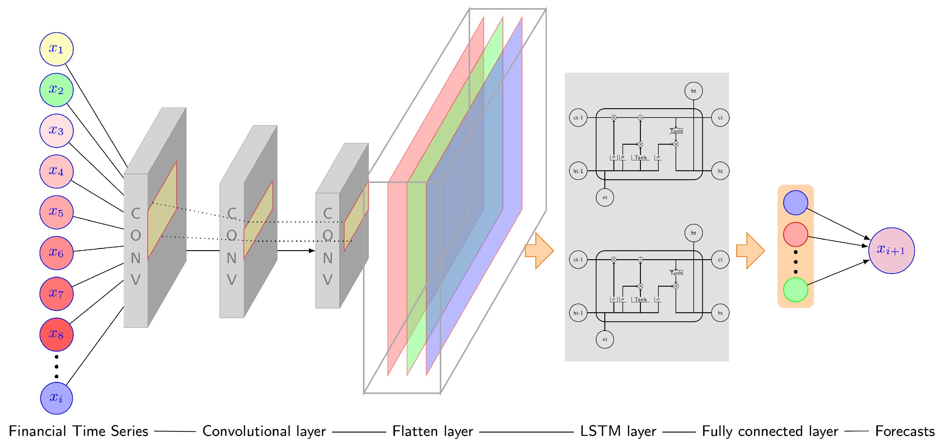
3. The ARMA-CNNLSTM Ensemble Forecasting Model

3.1. Ensemble Forecasting Model

Inspired by the unique advantages of the LSTM model and CNN model in the extraction of nonlinear features and the merits of the ARMA model in the extraction of linear features, the main idea of the ARMA-CNNLSTM model is to model and forecast the time series by applying individual models that can capture different data features (i.e., the ARMA model and CNN-LSTM model) and assigning corresponding weights to each model. The ARMA model and CNN-LSTM model are integrated into the ensemble framework to predict financial time series movements. In the proposed ARMA-CNNLSTM model, the linear ARMA model is used to capture the linear trend of the financial time series data and make linear predicted values for the time series, The CNN model and LSTM model are employed to build a nonlinear hybrid CNN-LSTM model, which is utilized to simultaneously extract the nonlinear spatial correlation features between the observed values at adjacent time points and the nonlinear long-term dependencies feature across the entire historical observations and then create nonlinear predicted values for the time series. At last, the final predicted values are constructed from the predicted values of the individual ensemble models, such as the linear predicted value of the ARMA model and the nonlinear predicted value of the CNN-LSTM model. They are calculated using the predicted values of each model with the weight coefficients corresponding to each model. In this paper, the linear predicted values and nonlinear predicted values are simply averaged to calculate the total forecast.
In the ARMA-CNNLSTM model, the forecasts from the individual ensemble models are assumed to be independent. The individual ensemble model assumes different data characteristics such as autocorrelation, spatial and temporal correlation. These data features may be classified into linear and nonlinear categories, which distinguishes them from each other during the modeling process.
The relationship between the total forecast y f ^ and the individual ensemble forecast y i ^ is assumed to be linear. Suppose that there are n individual ensemble forecasts and for each ensemble forecast in the total forecast of the weight w i , the final forecast y f ^ can be calculated as in Equation (1):
y f ^ = i = 1 n y i ^ w i

3.2. Individual Ensemble Models

As evidenced in the extant literature, there have been numerous models developed for financial time series forecasting. They need to be selected to construct an ensemble model pool that is capable of modeling a wide range of data features and produce a pool of individual ensemble forecasts y i .
As for the linear models, the representative ARMA model can be used to model the autocorrelation data feature. The ARMA model combines the features from the autoregressive (AR) model and moving average (MA) model to model the conditional means [34]. In the ARMA model, the current value of the time series data is determined linearly with the combination of its previous values and its previous white noise terms. The classical ARMA model is defined as in Equation (2):
ϕ ( L ) r t = μ + θ ( L ) u t w h e r e ϕ ( L ) = 1 ϕ 1 L ϕ 2 L 2 ϕ r L r θ ( L ) = 1 + θ 1 L + θ 2 L 2 + + θ m L m
where r t is a financial time series. u t is an independent, identically distributed series of random variables (RVs) ( i.e., white noise terms), μ is a constant, ϕ ( L ) represents the r-order lag polynomial of autoregression (AR), θ ( L ) represents the m-order lag polynomial of the moving average (MA), and L is the lag operator, which is used to convert the value of time point t 1 to the value of time point t. Given time series r t and integer k, the lag operator is defined as L k r t = r t k .
As for the nonlinear models, the widely popular deep learning model is the most promising one. Many deep learning models have been developed in the literature as the focus of machine learning modeling shifts from the increases in the number of neurons to the increases in the depth of the layers, and they target specific data features during the modeling process. The dominant ones include convolutional neural networks and long short-term memory networks. The design of the network structure in the deep learning model is flexible so that specialized layers in different deep learning models may be stacked together to model the diverse range of data characteristics. CNN-LSTM is one such model that contains layers for both the convolutional neural network and long short-term memory models. The CNN-LSTM model is used to model the spatial temporal data feature (i.e., it simultaneously extracts the nonlinear spatial correlation features between the observed values at adjacent time points and the nonlinear long-term temporal dependencies features across all historical observations). The typical CNN-LSTM network structure is illustrated in Figure 1.
The convolutional neural network (CNN) is one of the most popular deep learning models, being widely used to classify image data. With the introduction of the convolution operation in the convolutional layer, the CNN models the nonlinear relationship between the local regions of the input data [35]. The typical CNN model consists of several layers, such as the input layer, convolutional layer, pooling layer, flatten layer, fully connected layer, and output layer. The input layer feeds the input data into the convolutional layer. Then, the convolutional layer produces the feature maps containing targeted nonlinear data patterns from the input observations using filters in the convolutional layer. Neurons in the convolutional layer perform the convolution operations as in Equation (3) [28]:
F t = σ ( w x t + b )
where F t is the feature maps output from the filters in the convolutional layer, x t denotes the input matrix, w and b are the weight vector and bias vector of the filters, respectively, σ is the activation function, and * is the convolution operation.
The pooling layer is used to down-sample the feature maps generated by the previous convolutional layer. The flatten layer is applied to flatten the multidimensional feature maps’ shape into a one-dimensional shape and feed the transformed feature maps into the fully connected layer [29]. Then, the fully connected layer computes the final results according to these features. The calculation function is shown in Equation (4):
y t = ϕ ( w F t + b )
where y t is the final result at the current time point t, F t is the extracted features from the input data, w and b represent the weight vector and bias vector of the neurons in the fully connected layer, respectively, and ϕ is the activation function of a fully connected layer.
The long short-term memory (LSTM) network is a recent development in the recurrent neural network (RNN), which is known for its recurrent connection in the hidden layer design [36]. It has a feedback mechanism among different layers and has been extensively used to model the nonlinear temporal dependency patterns of time series. However, in practice, the RNN may encounter the vanishing gradients problem and exploding gradients problem in the training process of modeling the long-term dependencies of the time series [37]. The LSTM model is designed to tackle these drawbacks of the traditional RNN model. It has two loops in the LSTM hidden layer, which are the internal circulation system and the external circulation mechanism. The external circulation mechanism enables LSTM to recursively feed the LSTM hidden state at a prior time point in the network inputs and exert an impact on the final forecasting value [29]. The main part of the internal circulation system is the memory cell, which is a self-connecting unit. The internal circulation system controls the recurrent flow and updates the cell state information in the entire modeling process. The role of the memory cell is to store the temporal state information spanning long time sequences, and it also can prevent the exploding and vanishing gradient problems [38]. The memory cell is a critical part of the memory block, and the memory block is the basic structure of the hidden layer of LSTM. The memory block also includes three special adaptive multiplicative gate units, which work together to regulate the internal information flow in the memory block [37]. The input gate is used to decide which information from the current input can be fed into the memory cell to update the cell state. The function of the forget gate is to determine which information from the previous cell state could be stored in the memory cell and which sh ould be discarded. The forget gate can also prevent the value of the cell state from growing indefinitely. The role of the output gate is to control which information in the memory cell should be filtered out to compute the predicted value at the current time point. The values of the input gate, forget gate, and output gate as well as the candidate value of the memory cell are calculated as in Equation (5):
i t = σ ( w i [ x t , h t 1 ] + b i ) g t = σ ( w g [ x t , h t 1 ] + b g ) o t = σ ( w o [ x t , h t 1 ] + b o ) C t ^ = t a n h ( w c [ x t , h t 1 ] + b c )
where i t , g t , o t , and C t ^ are the values of the input gate, forget gate, output gate, and candidate cell state at time t, respectively. The parameters w t , w g , w o , and w c are the weight matrices of the corresponding units, and b t , b g , b o , and b c are the bias vectors of the corresponding units.
The state of the memory cell at the current time point t will be updated based on the values of the aforementioned input gate, forget gate, candidate memory cell, and previous memory cell state at time point t 1 as in Equation (6):
C t = g t C t 1 + i t C t ^
The symbol * is the element-wise product, C t 1 is the cell state at time point t 1 , and C t is the updated value of the cell state at the current time point t.
The output gate screens out the desired information from the memory cell, and the ultimate output value of the LSTM model is obtained according to the exported hidden state information from the memory block. The calculation processes of the hidden output state and final predicted value of LSTM are shown in Equation (7):
h t = o t t a n h ( C t ) y t = ϕ ( w y h t + b y )
where h t is the value of the hidden state of the memory block, y t is the final predicted value of the LSTM model, and w y and b y are the weight matrix and bias vector of the output layer of the LSTM model, respectively. In these above-mentioned equation, σ is the sigmoid function, t a n h is the hyperbolic tangent function, and ϕ is the activation function of the LSTM output layer. The parameters of the LSTM model will be optimized by minimizing the loss function using the backpropagation algorithm based on gradient descent in the training process [39].

4. Empirical Studies

4.1. Data Description and Statistical Tests

In this paper, different financial time series data are used to conduct the empirical evaluation of the predictive accuracy of the proposed ARMA-CNNLSTM forecasting model. Due to data availability, these included weekly EU ETS data in the European carbon trading market, the daily Shanghai composite index in the Chinese stock market, and daily Bitcoin prices in the cryptocurrency market. The reasons for the choice of these time series in these three representative financial markets are as follows. The European Union Emission Trading System (EU ETS) is the largest financial trading market in the world, with the total market value being about USD 148 billion, roughly 84% of the global financial market [7,19]. The EU ETS has attracted the attention of a large number of market participants such as investors, traders, and brokers around the world. The Shanghai stock index is one of the major stock indexes in China, attracting the attention of a large number of stock market participants, and its trading volume has grown rapidly in recent years. It is of great significance to forecast the Shanghai stock index’s price movement. Bitcoin has been regarded as one of the most important cryptocurrencies in the global virtual currency market [4,40]. It has gradually attracted more and more attention from investors, policymakers, and the media [22].
The data sources were netease finance, sandbag, and investing websites, which all provided publicly available datasets. The EU ETS dataset covered the periods from 7 April 2008 to 21 September 2020, with a total of 645 weekly observations. The Shanghai Composite index dataset covered the period from 4 January 2010 to 23 January 2020, which contained 2447 daily observations. The Bitcoin dataset covered the period from 2 February 2012 to 8 August 2020, which contained 3107 daily observations. All datasets were split into training and test datasets using the conventional 80:20 ratio to facilitate the model testing and performance evaluations. The training set was used to train the parameters of different models, and the testing set was utilized to test the predictive accuracy of different models in out-of-sample forecasting exercises [37]. The performance of the models was evaluated using mainstream predictive accuracy measures, such as the mean absolute error (MAE), mean absolute percentage error (MAPE), root mean square error (RMSE), and directional prediction statistic D s t a t . The MAE, MAPE, and RMSE were used to measure the distance between the predicted value and the actual value. The smaller the values for the MAE, MAPE, and RMSE were, the closer the predicted value was to the actual value, and the better the predicted performance of the forecasting model was D s t a t measured the accuracy of the forecasting models in predicting the direction of financial time series movement. The larger the value of D s t a t was, the more accurate the forecasting model was in predicting the direction of financial time series movement. Both random walk (RW) and ARMA models were used as the benchmark models in this paper.
The descriptive statistics and the p-values of the BDS test of independence and Jarque–Bera test of normality are reported for the EU ETS financial futures prices, the closing value of the Shanghai stock index, and the closing prices of Bitcoin in Table 1.
The results in Table 1 show that the distribution of the EU ETS financial futures prices, Shanghai stock index, and Bitcoin prices deviated from the normal distribution, as the kurtosis value deviates from 3. There was significant volatility in the financial time series movement, indicated by the standard deviation value. We used the augmented Dickey–Fuller (ADF) test, a popular nonstationarity test, to test for the stationarity property in the financial time series data. The ADF test of the Shanghai stock index rejected the null hypothesis, as its p-value of 0.001 was less than the cut-off value of 0.05. The original financial time series was transformed using the first difference operation. The EU ETS financial futures prices were not stationary, as the null hypothesis could not be rejected at a p-value of 0.4685, and the Bitcoin closing prices were not stationary, as the null hypothesis could not be rejected at a p-value of 0.5312, which was significantly higher than the cut-off value of 0.05.

4.2. Results for In-Sample Model Fit

We searched for and determined the optimal parameters for the benchmark ARMA model, individual model, and ARMA-CNNLSTM model. We applied these models to forecast the financial time series using the validation set. The ARMA model was considered the benchmark model in this paper since, until now there has been no conclusive evidence that any econometric models consistently beat these two benchmark models [41]. It is widely considered the most robust baseline model in the literature. There are several hyperparameters for the MLP, CNN, and LSTM models, such as the number of filters in the CNN layer, the number of hidden neurons in the LSTM hidden layer, the number of neurons in the fully connected layer, the learning rate, and the training epochs. We used the grid search method to search for the value of the optimal parameter. The lower and upper bounds for the search space were as follows: filters (1, 10) and neurons (1, 100). In these artificial intelligence models, the search scope of the hidden layers was from 1 to 2, and the search scope of the neurons in each hidden layer was from 1 to 200. The rolling window was set to five, which means that each sub-period was fed into the artificial intelligence models containing five previous observations. This is equivalent to 5 trading days in a week. To make a one-step-ahead prediction, the rolling windows scrolled forward one step each time. The last 10% of the dataset in the training set was taken as the validation set. Through the greedy search method, the optimal model structure was determined by evaluating the RMSE values of different model structures in the validation set. We illustrate the performance of the ARMA-CNNLSTM model using different parameters in Figure 2, Figure 3 and Figure 4.
The performance of the model errors can be seen clearly from Figure 2, Figure 3 and Figure 4. When different sets of parameters were used for the CNN and LSTM models, we used the RMSE as the performance measure and adopted the minimization criteria. The parameters with which the ARMA-CNNLSTM model generated the smallest MSE were chosen as the optimal parameters. The optimal model parameters were as follows. Based on the minimization of Akaike’s Information Criterion (AIC), the ARMA (1,1) model was selected for EU ETS and Shanghai stock index while ARMA(1,0) was selected for Bitcoin. In the prediction process, we set the rolling window size of the ARMA model equal to the amount of training data, and the financial time series were predicted by scrolling forward one step for each time of the rolling window.
For EU ETS, the network structure and parameters for the MLP model were set as follows: dense layer (units = 78, activation = ReLU)–dense layer (units = 78, activation = ReLU)–dense layer (units = 78, activation = ReLU)–dropout layer (0.5)–dense layer (units = 1). The network structure and parameters for the LSTM model were set as follows: LSTM layer (units = 86, activation = ReLU)–LSTM layer (units = 86, activation = ReLU)–dropout layer (0.5)–dense layer (units = 1). The network structure and parameters for the CNN were set as follows: convolution layer (filters = 10, kernel size = 2, activation = ReLU)–convolution layer (filters = 10, kernel size = 2, activation = ReLU)–convolution layer (filters = 10, kernel size = 2, activation = ReLU)–pooling layer (max pooling, pooling size = 2)–flatten Layer–dense layer (units = 81, activation = ReLU)–dropout layer (0.5)–dense layer (units = 1). The network structure and parameters for the ARMA-CNNLSTM model were set as follows: CNN layer (filters = 3, kernel size = 2, activation = ReLU)–CNN layer (filters = 3, kernel size = 2, activation = ReLU)–CNN layer (filters = 3, kernel size = 2, activation = ReLU)–pooling layer (max pooling, pooling size = 2)–flatten layer–LSTM layer (units = 20, activation = ReLU)–dropout layer (0.5)–dense layer (units = 10, activation = ReLU)–dropout layer (0.2)–dense layer (units = 1).
For Shanghai stock index, the network structure and parameters for the MLP model were set as follows: dense layer (units = 80, activation = ReLU)–dense layer (units = 80, activation = ReLU)–dropout layer (0.5)–dense layer (units = 1). The network structure and parameters for the LSTM model were set as follows: LSTM layer (units = 3, activation = ReLU)–dropout layer (0.5)–dense layer (units = 1). The network structure and parameters for the CNN were set as follows: convolution layer (filters = 8, kernel size = 4, activation = ReLU)–pooling layer (max pooling, pooling size = 2)–dense layer (units = 75, activation = ReLU)–dropout layer (0.5)–dense layer (units = 1). The network structure and parameters for the ARMA-CNNLSTM model were set as follows: CNN layer (filters = 3, kernel size = 2, activation = ReLU)–CNN layer (filters = 3, kernel size = 2, activation = ReLU)–CNN layer (filters = 3, kernel size = 2, activation = ReLU)–pooling layer (max pooling, pooling size = 2)–flatten layer–LSTM layer (units = 72, activation = ReLU)–LSTM layer (units = 72, activation = ReLU)–dropout layer (0.5)–dense layer (units = 10, activation = ReLU)–dropout layer (0.2)–dense layer (units = 1).
For Bitcoin, dense layer (units = 61, activation = ReLU)–dense layer (units = 61, activation = ReLU)–dense layer (units = 61, activation = ReLU)–dropout layer (0.5)–dense layer (units = 1). The network structure and parameters for the LSTM model were set as follows: LSTM layer (units = 31, activation = ReLU)–LSTM layer (units = 31, activation = ReLU)–dropout layer (0.5)–dense layer (units = 1). The network structure and parameters for the CNN were set as follows: convolution layer (filters = 5, kernel size = 2, activation = ReLU)–convolution layer (filters = 5, kernel size = 2, activation = ReLU)–convolution layer (filters = 5, kernel size = 2, activation = ReLU)–pooling layer (max pooling, pooling size = 2)–dense layer (units = 73, activation = ReLU)–dropout layer (0.5)–dense layer (units = 1). The network structure and parameters for the ARMA-CNNLSTM model were set as follows: CNN layer (filters = 5, kernel size = 2, activation = ReLU)–CNN layer (filters = 5, kernel size = 3, activation = ReLU)–pooling layer (max pooling, pooling size = 2)–flatten layer–LSTM layer (units = 17, activation = ReLU)–dropout layer (0.5)–dense layer (units = 10, activation = ReLU)–dropout layer (0.2)–dense layer (units = 1). For the MLP, CNN, LSTM, and ARMA-CNNLSTM models, the learning rate was 0.001.

4.3. Results for Out-of-Sample Model Performance Evaluation

With the determined optimal parameters, the benchmark model, as well as the ARMA-CNNLSTM model, were applied to the forecasting of financial time series using the out-of-sample dataset. The performances of these models were compared and evaluated. Table 2 shows the predictive performances of different forecasting models for the EU ETS financial time series based on different evaluation criteria. Table 3 shows the predictive performances of different prediction models based on different evaluation criteria for the Shanghai stock index. Table 4 shows the predictive performance of different prediction models based on different evaluation criteria for Bitcoin’s closing prices.
The results in Table 2 show that the ARMA-CNNLSTM model achieved a better predictive performance than all the other benchmark models and individual models in terms of the four predictive performance measures. The RMSE, MAPE, and MAE of the ARMA-CNNLSTM model were all lower than those of the random walk and ARMA models, which indicates that the ARMA-CNNLSTM model produced financial time series forecasts with a higher level of forecasting accuracy than the mainstream models. The statistical measure D s t a t for the ARMA-CNNLSTM model forecasts was higher than those of all the other models, which indicates that the forecasts from the ARMA-CNNLSTM models provided a higher level of directional forecasting accuracy than those of the benchmark models as well as the mainstream models. From the results in Table 3, the RMSE, MAPE, and MAE of the ARMA-CNNLSTM model were lower than the random walk, ARMA, CNN, and LSTM models, indicating the ARMA-CNNLSTM model for the Shanghai stock index time series outperformed the benchmark and individual models with a higher forecasting accuracy. The statistical measure D s t a t for the ARMA- CNNLSTM model forecasts was higher than for the CNN model, MLP model, and random walk model, which shows that the ARMA-CNNLSTM model had a better direction prediction accuracy than the mainstream models. The results in Table 4 indicate that the ARMA-CNNLSTM model showed a better forecasting accuracy for Bitcoin’s closing prices than the benchmark and mainstream models, based on the lower values for the RMSE, MAPE, and MAE of the ARMA-CNNLSTM model. The statistical measure D s t a t for the ARMA-CNNLSTM model forecasts was higher than those for the benchmark models as well as the mainstream models, which illustrates that the ARMA-CNNLSTM model provided a higher level of directional forecasting accuracy than those of all the other models.
Interestingly, we found that neither the CNN nor LSTM forecasts dominated the benchmark random walk and ARMA models. This shows that as these two models focus on certain data features, neither of these two deep learning models can provide an adequate fit for financial data with complex data features. They only model certain aspects of the data characteristics with their unique assumptions. The mixture of diverse data features in the empirical data requires the integration and combination of different deep learning models, such as the proposed ARMA-CNNLSTM model in the ensemble framework. The worse performance of the individual CNN and LSTM models could also be attributed to the suboptimal hyperparameter optimization process. In the literature, hyperparameter optimization is a difficult research problem. Although more advanced optimization models such as genetic algorithms have been introduced to search for the optimal hyperparameters, there is a lack of consensus on the best optimization model in the literature. The simple averaging method serves as a robust linear ensemble method and has been adopted in this paper to construct the ARMA-CNNLSTM model.
Meanwhile, the improved forecasting accuracy of the ARMA-CNNLSTM model was attributed to the introduction of deep learning models focusing on different data features so that the forecasts from the ARMA and CNN-LSTM models assumed different data features and had a higher level of independence. forecasts from the ARMA and CNN-LSTM models to average the individual forecasts would reduce the estimation bias and improve the forecasting accuracy. The ensemble model incorporates the partial information captured by the individual deep learning models and econometric models effectively.

5. Conclusions

In this paper, we proposed a new ensemble forecasting model based on the ARMA model and CNN-LSTM model. We found that different deep learning models target different data characteristics with their unique assumptions and network structure, and they are better at recognizing and modeling different nonlinear data features, such as spatial and temporal data features. The ensemble of individual forecasts of both the ARMA and CNN-LSTM models effectively reduced the estimation bias and improved the forecasting accuracy. In this research, the ARMA-CNNLSTM model had the best predictive ability in financial time series forecasting when it was compared with the baseline models.
The work in this paper has profound implications. In this paper, the ARMA-CNNLSTM model was applied extensively to three representative financial time series with widely different volatility levels and characteristics. It achieved consistent, superior performance. This demonstrates the robustness of the ARMA-CNNLSTM model and the potential of this model to be generalized beyond the dataset investigated in this paper to a diverse range of financial time series in practice. What is more, our results imply that by modeling different financial time series data features with specific deep learning models, it is possible to improve the predictive capability of the forecasting model. Although the deep learning models demonstrated overwhelming success in modeling the nonlinear data features, we found through a comprehensive comparative empirical study that they may not model the complex data features well, possibly due to the difficulty of setting the correct hyperparameters for the mixture of linear and nonlinear data features during the model’s tuning process. The introduction of the deep learning model into the ensemble framework can contribute significantly to the understanding and modeling of the mixture of data features. Given the rapid development in deep learning fields, it is expected that the modeling accuracy of the nonlinear data features, such as the spatiotemporal data features, will improve continuously, and this would also lead to improvement in the ensemble model. Therefore, future research can be directed toward this aspect, where both the introduction of a more innovative deep learning model and the design of a new optimization algorithm for the ensemble model offer promising approaches to forecasting performance improvement.

Author Contributions

Conceptualization, K.H., L.J. and Y.Z.; methodology, L.J. and Y.Z.; writing—original draft preparation, K.H., L.J. and Q.Y.; writing—review and editing, Y.Z., Q.Y. and J.P.; funding acquisition, K.H. and J.P. All authors have read and agreed to the published version of the manuscript.

Funding

This research was funded by the National Natural Science Foundation of China (grant number 72271089 and grant number 71671013), Hunan Provincial Natural Science Foundation of China (grant number 2022JJ30401), and the National Social Science Fund of China (grant number 18BJL105).

Data Availability Statement

Publicly available datasets were analyzed in this study. These data can be found here: https://quotes.money.163.com, https://sandbag.org.uk, https://cn.investing.com (accessed on 1 October 2020).

Conflicts of Interest

The authors declare no conflict of interest.

References

  1. Kim, H.Y.; Won, C.H. Forecasting the volatility of stock price index: A hybrid model integrating LSTM with multiple GARCH-type models. Expert Syst. Appl. 2018, 103, 25–37. [Google Scholar] [CrossRef]
  2. Dash, R.; Dash, P.K. A hybrid stock trading framework integrating technical analysis with machine learning techniques. J. Financ. Data Sci. 2016, 2, 42–57. [Google Scholar] [CrossRef] [Green Version]
  3. Wang, J.J.; Wang, J.Z.; Zhang, Z.G.; Guo, S.P. Stock index forecasting based on a hybrid model. Omega 2012, 40, 758–766. [Google Scholar] [CrossRef]
  4. Chen, Z.; Li, C.; Sun, W. Bitcoin price prediction using machine learning: An approach to sample dimension engineering. J. Comput. Appl. Math. 2020, 365, 112395. [Google Scholar] [CrossRef]
  5. Leonardo Ranaldi, M.G.F.F. CryptoNet: Using Auto-Regressive Multi-Layer Artificial Neural Networks to Predict Financial Time Series. Information 2022, 13, 524. [Google Scholar] [CrossRef]
  6. Xu, H.; Wang, M.; Jiang, S.; Yang, W. Carbon price forecasting with complex network and extreme learning machine. Phys. Stat. Mech. Its Appl. 2019, 545, 122830. [Google Scholar] [CrossRef]
  7. Atsalakis, G.S. Using computational intelligence to forecast carbon prices. Appl. Soft Comput. J. 2016, 43, 107–116. [Google Scholar] [CrossRef]
  8. Daskalakis, G. On the efficiency of the European carbon market: New evidence from Phase II. Energy Policy 2013, 54, 369–375. [Google Scholar] [CrossRef]
  9. Nayak, S.C.; Misra, B.B.; Behera, H.S. Artificial chemical reaction optimization of neural networks for efficient prediction of stock market indices. Ain Shams Eng. J. 2017, 8, 371–390. [Google Scholar] [CrossRef] [Green Version]
  10. Zhu, B.; Wei, Y. Carbon price forecasting with a novel hybrid ARIMA and least squares support vector machines methodology. Omega 2013, 41, 517–524. [Google Scholar] [CrossRef]
  11. Rout, A.K.; Dash, P.K.; Dash, R.; Bisoi, R. Forecasting financial time series using a low complexity recurrent neural network and evolutionary learning approach. J. King Saud Univ.-Comput. Inf. Sci. 2017, 29, 536–552. [Google Scholar] [CrossRef] [Green Version]
  12. Rounaghi, M.M.; Nassir Zadeh, F. Investigation of market efficiency and Financial Stability between S&P 500 and London Stock Exchange: Monthly and yearly Forecasting of Time Series Stock Returns using ARMA model. Phys. A Stat. Mech. Its Appl. 2016, 456, 10–21. [Google Scholar] [CrossRef]
  13. Shafie-khah, M.; Moghaddam, M.P.; Sheikh-El-Eslami, M.K. Price forecasting of day-ahead electricity markets using a hybrid forecast method. Energy Convers. Manag. 2011, 52, 2165–2169. [Google Scholar] [CrossRef]
  14. Pai, P.F.; Lin, C.S. A hybrid ARIMA and support vector machines model in stock price forecasting. Omega 2005, 33, 497–505. [Google Scholar] [CrossRef]
  15. Zhang, L.; Zhang, J.; Xiong, T.; Su, C. Interval Forecasting of Carbon Futures Prices Using a Novel Hybrid Approach with Exogenous Variables. Discret. Dyn. Nat. Soc. 2017, 2017, 5730295. [Google Scholar] [CrossRef] [Green Version]
  16. Ibrahim, A.; Kashef, R.; Corrigan, L. Predicting market movement direction for bitcoin: A comparison of time series modeling methods. Comput. Electr. Eng. 2021, 89, 106905. [Google Scholar] [CrossRef]
  17. Chevallier, J. Nonparametric modeling of carbon prices. Energy Econ. 2011, 33, 1267–1282. [Google Scholar] [CrossRef]
  18. Zhao, X.; Han, M.; Ding, L.; Kang, W. Usefulness of economic and energy data at different frequencies for carbon price forecasting in the EU ETS. Appl. Energy 2018, 216, 132–141. [Google Scholar] [CrossRef]
  19. Fan, X.; Li, S.; Tian, L. Chaotic characteristic identification for carbon price and an multi-layer perceptron network prediction model. Expert Syst. Appl. 2015, 42, 3945–3952. [Google Scholar] [CrossRef]
  20. Fenghua, W.; Jihong, X.; Zhifang, H.E.; Xu, G. Stock Price Prediction based on SSA and SVM. Procedia Comput. Sci. 2014, 31, 625–631. [Google Scholar] [CrossRef] [Green Version]
  21. Shen, G.; Tan, Q.; Zhang, H.; Zeng, P.; Xu, J. Deep Learning with Gated Recurrent Unit Networks for Financial Sequence Predictions. Procedia Comput. Sci. 2018, 131, 895–903. [Google Scholar] [CrossRef]
  22. Atsalakis, G.S.; Atsalaki, I.G.; Pasiouras, F.; Zopounidis, C. Bitcoin price forecasting with neuro-fuzzy techniques. Eur. J. Oper. Res. 2019, 276, 770–780. [Google Scholar] [CrossRef]
  23. Nagula, P.K.; Alexakis, C. A new hybrid machine learning model for predicting the bitcoin (BTC-USD) price. J. Behav. Exp. Financ. 2022, 36, 100741. [Google Scholar] [CrossRef]
  24. Sun, G.; Chen, T.; Wei, Z.; Sun, Y.; Zang, H.; Chen, S. A Carbon Price Forecasting Model Based on Variational Mode Decomposition and Spiking Neural Networks. Energies 2016, 9, 54. [Google Scholar] [CrossRef] [Green Version]
  25. Zhu, B.; Ye, S.; Wang, P.; He, K.; Zhang, T.; Wei, Y.M. A novel multiscale nonlinear ensemble leaning paradigm for carbon price forecasting. Energy Econ. 2018, 70, 143–157. [Google Scholar] [CrossRef]
  26. Zhu, B.; Han, D.; Wang, P.; Wu, Z.; Zhang, T.; Wei, Y.M. Forecasting carbon price using empirical mode decomposition and evolutionary least squares support vector regression. Appl. Energy 2017, 191, 521–530. [Google Scholar] [CrossRef] [Green Version]
  27. Ni, L.; Li, Y.; Wang, X.; Zhang, J.; Yu, J.; Qi, C. Forecasting of Forex Time Series Data Based on Deep Learning. Procedia Comput. Sci. 2019, 147, 647–652. [Google Scholar] [CrossRef]
  28. Long, W.; Lu, Z.; Cui, L. Deep learning-based feature engineering for stock price movement prediction. Knowl.-Based Syst. 2019, 164, 163–173. [Google Scholar] [CrossRef]
  29. Gonçalves, R.; Ribeiro, V.M.; Pereira, F.L.; Rocha, A.P. Deep learning in exchange markets. Inf. Econ. Policy 2019, 47, 38–51. [Google Scholar] [CrossRef]
  30. Peng, L.; Liu, S.; Liu, R.; Wang, L. Effective long short-term memory with differential evolution algorithm for electricity price prediction. Energy 2018, 162, 1301–1314. [Google Scholar] [CrossRef]
  31. Cen, Z.; Wang, J. Crude oil price prediction model with long short term memory deep learning based on prior knowledge data transfer. Energy 2019, 169, 160–171. [Google Scholar] [CrossRef]
  32. Zhang, G.P. Time series forecasting using a hybrid ARIMA and neural network model. Neurocomputing 2003, 50, 159–175. [Google Scholar] [CrossRef]
  33. Jeong, K.; Koo, C.; Hong, T. An estimation model for determining the annual energy cost budget in educational facilities using SARIMA (seasonal autoregressive integrated moving average) and ANN (artificial neural network). Energy 2014, 71, 71–79. [Google Scholar] [CrossRef]
  34. Brooks, C. Introductory Econometrics for Finance, 2nd ed.; Cambridge University Press: Cambridge, UK; New York, NY, USA, 2008. [Google Scholar]
  35. Li, X.; Shang, W.; Wang, S. Text-based crude oil price forecasting: A deep learning approach. Int. J. Forecast. 2019, 35, 1548–1560. [Google Scholar] [CrossRef]
  36. Sepp Hochreiter and Jürgen Schmidhuber. Long Short-Term Memory. Neural Comput. 1997, 9, 1735–1780. [Google Scholar] [CrossRef] [PubMed]
  37. Liu, Y.; Yang, C.; Huang, K.; Gui, W. Non-ferrous metals price forecasting based on variational mode decomposition and LSTM network. Knowl.-Based Syst. 2019, 105006. [Google Scholar] [CrossRef]
  38. Cao, J.; Li, Z.; Li, J. Financial time series forecasting model based on CEEMDAN and LSTM. Phys. A Stat. Mech. Appl. 2019, 519, 127–139. [Google Scholar] [CrossRef]
  39. Qing, X.; Niu, Y. Hourly day-ahead solar irradiance prediction using weather forecasts by LSTM. Energy 2018, 148, 461–468. [Google Scholar] [CrossRef]
  40. Sun, X.; Liu, M.; Sima, Z. A novel cryptocurrency price trend forecasting model based on LightGBM. Financ. Res. Lett. 2020, 32, 101084. [Google Scholar] [CrossRef]
  41. Alquist, R.; Kilian, L. What Do We Learn from the Price of Crude Oil Futures? J. Appl. Econom. 2010, 25, 539–573. [Google Scholar] [CrossRef] [Green Version]
Figure 1. CNN-LSTM network structure.
Mathematics 11 01054 g001
Figure 2. RMSE of ARMA-CNNLSTM forecasts using different model parameters in the validation set of EU ETS financial time series forecasting.
Mathematics 11 01054 g002
Figure 3. RMSE of ARMA-CNNLSTM forecasts using different model parameters in the validation set of Shanghai stock index forecasting.
Mathematics 11 01054 g003
Figure 4. RMSE of ARMA-CNNLSTM forecasts using different model parameters in the validation set of Bitcoin closing prices forecasting.
Mathematics 11 01054 g004
Table 1. Descriptive statistics and statistical tests of three financial time series.
DatasetMeanMinMaxStandard DeviationSkewnessKurtosis p B D S p A D F
P E U E T S 12.322.9730.527.400.772.3400.4685
P S S I 2801.71950.015166.35529.380.754.5300.001
P B i t c o i n 3028.114.22191873847.121.153.2500.5312
Table 2. Comparison of the predictive abilities of different models for EU ETS financial time series.
ModelRMSEMAPEMAE D s t a t
Random walk1.23990.04150.91510.4651
ARMA1.23790.04130.91220.5581
MLP1.37710.04661.02170.5039
LSTM3.98670.15523.36960.5504
CNN1.77480.06211.34740.4884
ARMA-CNNLSTM1.21950.04000.88370.6047
Table 3. Comparison of the predictive abilities of different models for Shanghai stock index time series.
ModelRMSE × 10 2 MAPEMAE × 10 2 D s t a t
Random walk1.71735.62311.2710.3517
ARMA1.20041.38530.86690.7526
MLP1.21751.22910.87270.7321
LSTM1.20221.06370.86550.7464
CNN1.20611.20570.86790.7403
ARMA-CNNLSTM1.19641.14790.8610.7423
Table 4. Comparison of the predictive abilities of different models for Bitcoin’s closing prices.
ModelRMSEMAPEMAE D s t a t
Random walk323.83110.0257199.14240.5314
ARMA324.67880.0258199.52870.4928
MLP341.06480.028217.34720.5153
LSTM476.84390.0423327.07950.5395
CNN378.660.0315243.0130.5298
ARMA-CNNLSTM323.77050.0254197.040.5556
Disclaimer/Publisher’s Note: The statements, opinions and data contained in all publications are solely those of the individual author(s) and contributor(s) and not of MDPI and/or the editor(s). MDPI and/or the editor(s) disclaim responsibility for any injury to people or property resulting from any ideas, methods, instructions or products referred to in the content.

