Article

On Some Solvable Systems of Some Rational Difference Equations of Third Order

by
Khalil S. Al-Basyouni
1 and
Elsayed M. Elsayed
1,2,*
1
Faculty of Science, Mathematics Department, King Abdulaziz University, P.O. Box 80203, Jeddah 21589, Saudi Arabia
2
Department of Mathematics, Faculty of Science, Mansoura University, Mansoura 35516, Egypt
*
Author to whom correspondence should be addressed.
Mathematics 2023, 11(4), 1047; https://doi.org/10.3390/math11041047
Submission received: 19 January 2023 / Revised: 15 February 2023 / Accepted: 17 February 2023 / Published: 19 February 2023

Abstract

:
Our aim in this paper is to obtain formulas for solutions of rational difference equations such as x n + 1 = 1 ± x n 1 y n / 1 y n , y n + 1 = 1 ± y n 1 x n / 1 x n , and x n + 1 = 1 ± x n 1 y n 2 / 1 y n , y n + 1 = 1 ± y n 1 x n 2 / 1 x n , where the initial conditions x 2 , x 1 , x 0 , y 2 , y 1 , y 0 are non-zero real numbers. In addition, we show that the some of these systems are periodic with different periods. We also verify our theoretical outcomes at the end with some numerical applications and draw it by using some mathematical programs to illustrate the results.

1. Introduction

Nonlinear difference equations have recently captured the attention of numerous scholars. In fact, during the past ten years, we have encouraged a rapid rise in interest in these kinds of equations. The fact that these types of equations have several applications not just in mathematics but also in related areas, particularly in biological sciences, engineering, ecology, discrete temporal systems, economics, physics, and so on, may have contributed to the desire. We believe that, as more appealing and engaging results are achieved and communicated in studies, this area of research will continue to captivate the minds of more scholars in the years to come. The challenge of solving nonlinear difference equations in closed form has emerged as a common theme in this research area. In reality, a large number of articles attempt to solve nonlinear difference equations in any way they can; for an example, see [1,2,3,4,5,6]. Evidently, it can be very difficult to obtain the solution form for these kinds of equations in general. However, a number of approaches have lately been proposed to simplify challenging nonlinear difference equations into linear forms with established solution forms. For instance, a sizable class of nonlinear difference equations were solved in closed-form by converting into linear types (see, e.g., [7,8,9,10,11,12]).
Numerous academics have examined how systems of solved difference equations behave, for instance: Cinar examined the answers to the following system of difference equations in [13].
Ψ n + 1 = m Θ n , Θ n + 1 = p Θ n Ψ n 1 Θ n 1 .
El-Metwally [14] found the solutions form for the following systems of rational difference equations:
μ n + 1 = μ n 1 ϖ n ± μ n 1 ± ϖ n 2 , ϖ n + 1 = ϖ n 1 μ n ± ϖ n 1 ± μ n 2 .
Kara and Yazlik in [15] showed that the following three-dimensional system of difference equations
ϖ n + 1 = ϑ n ϑ n 2 b ϖ n 1 + a ϑ n 2 , ϑ n + 1 = z n z n 2 d ϑ n 1 + c z n 2 , z n + 1 = ϖ n ϖ n 2 f z n 1 + e ϖ n 2 ,
can be solved. Furthermore, they determined the forbidden set of the initial conditions by employing acquired formulas. Finally, they provided various applications involving the difference equation system discussed before.
Mansour et al. [16] examined the behavior of the difference equations systems’ solutions
ϖ n + 1 = ϖ n 5 1 + ϖ n 5 y n 2 , y n + 1 = y n 5 ± 1 ± y n 5 ϖ n 2 .
In [17], Ozban studied the positive solutions of the following system of rational difference equations
ϖ n + 1 = a ϑ n 3 , ϑ n + 1 = b ϑ n 3 ϖ n q ϑ n p .
Sroysang [18] focused on a system of a rational higher-order difference equation
x n + 1 = x n m + 1 A + ϑ n ϑ n 1 ϑ n m + 1 , ϑ n + 1 = ϑ n m + 1 A + x n x n 1 x n m + 1 .
Touafek et al. [19] investigated the periodic nature and provided the form of the solutions of the following systems of rational difference equations
x n + 1 = y n x n 1 ( ± 1 ± y n ) , y n + 1 = x n y n 1 ( ± 1 ± x n ) .
Furthermore, Yalçınkaya [20] has obtained the sufficient conditions for the global asymptotic stability of the following system of two nonlinear difference equations
x n + 1 = x n + y n 1 x n y n 1 1 , y n + 1 = y n + x n 1 y n x n 1 1 .
In [21], Zhang et al. studied the boundedness, the persistence, and global asymptotic stability of the positive solutions of the following system
x n = A + 1 y n p , y n = A + y n 1 x n r y n s .
Zhang et al. [22] studied the dynamics of a system of the rational third-order difference equation
x n + 1 = x n 2 B + y n y n 1 y n 2 , y n + 1 = y n 2 A + x n x n 1 x n 2 .
For more studies for nonlinear difference equations and systems of rational difference equations see [2,23,24,25,26,27,28,29,30,31,32].
Furthermore, difference equations are appropriate models for describing situations where population growth is not continuous but seasonal with overlapping generations.
Researchers have looked at the generalized Beverton–Holt stock recruitment model in [33]
x n + 1 = a x n + b x n 1 1 + c x n 1 + d x n .
Khaliq et al. [34] studied the dynamical analysis of the following system of discrete-time two-predators and the one-prey Lotka–Volterra model
x n + 1 = α x n β x n y n γ x n z n 1 + δ x n , y n + 1 = ζ y n + η x n y n μ y n z n 1 + ε y n , z n + 1 = v z n + ρ x n z n σ y n z n 1 + ω z n .
The boundedness character, persistence, local, and global behavior of the following two-directional interacting and invasive species model were examined by Din and Elsayed [35]
x n + 1 = α + β x n + γ x n 1 e y n , y n + 1 = δ + ϵ y n + ζ y n 1 e x n .
The authors in [36] explored local dynamics with topological classifications, bifurcation analysis, and chaos control in a discrete-time COVID-19 epidemic model. See also [37,38,39].
In this paper, we deal with the existence of the form for the solutions of the following systems of difference equations
x n + 1 = 1 + δ x n 1 y n 1 y n , y n + 1 = 1 + γ y n 1 x n 1 x n ,
and
x n + 1 = 1 + δ x n 1 y n 2 1 y n , y n + 1 = 1 + γ y n 1 x n 2 1 x n ,
with the initial conditions x 2 , x 1 , x 0 , y 2 , y 1 , and y 0 are arbitrary non zero real numbers.

2. Main Results

2.1. System (1) When δ = +1 and γ = +1

In this section, we investigate the solutions of the following system of two difference equations
x n + 1 = 1 + x n 1 y n 1 y n , y n + 1 = 1 + y n 1 x n 1 x n ,
where n N 0 and the initial conditions are arbitrary non zero real numbers with x 0 1 and y 0 1 .
Theorem 1.
Let x n , y n n = 1 be a solution of System (1), then
1. 
x n , y n n = 1 is a periodic solution with period four, i.e., x n + 4 = x 4 , y n + 4 = y n for all n 1 .
2. 
x n , y n n = 2 has the following form
x 4 n 1 = x 1 , x 4 n = x 0 , x 4 n + 1 = 1 + x 1 y 0 1 y 0 , x 4 n + 2 = ( x 0 1 ) ( 1 y 1 ) y 1 , y 4 n 1 = y 1 , y 4 n = y 0 , y 4 n + 1 = 1 + y 1 x 0 1 x 0 , y 4 n + 2 = ( x 1 1 ) ( 1 y 0 ) x 1 .
Proof. 
From Equation (1), we have
x n + 1 = 1 + x n 1 y n 1 y n , y n + 1 = 1 + y n 1 x n 1 x n , x n + 2 = 1 + x n y n + 1 1 y n + 1 = 1 + x n 1 + y n 1 x n 1 x n 1 1 + y n 1 x n 1 x n = 1 + x n 1 + y n 1 x n 1 x n y n 1 x n 1 x n = 1 x n 1 x n + y n 1 x n y n 1 x n = y n 1 1 x n + y n 1 x n y n 1 = y n 1 1 + x n y n 1 x n y n 1 = ( x n 1 ) ( 1 y n 1 ) y n 1 , y n + 2 = 1 + y n x n + 1 1 x n + 1 = 1 + y n 1 + x n 1 y n 1 y n 1 1 + x n 1 y n 1 y n = 1 1 + x n 1 y n 1 y n x n 1 1 y n = 1 1 y n + x n 1 y n x n 1 = x n 1 1 y n + x n 1 y n x n 1 = ( x n 1 1 ) ( 1 y n ) x n 1 .
Furthermore, we see from Equation (1) that
x n + 3 = 1 + x n + 1 y n + 2 1 y n + 2 = 1 + 1 + x n 1 y n 1 y n ( x n 1 1 ) ( 1 y n ) x n 1 1 ( x n 1 1 ) ( 1 y n ) x n 1 = 1 + 1 y n + x n 1 y n ( x n 1 1 ) x n 1 x n 1 1 ) ( 1 y n = 1 + 1 y n + x n 1 y n ( x n 1 1 ) x n 1 x n 1 1 + y n x n 1 y n = 1 + 1 y n + x n 1 y n ( x n 1 1 ) 1 y n + x n 1 y n = 1 + ( x n 1 1 ) = x n 1 , y n + 3 = 1 + y n + 1 x n + 2 1 x n + 2 = 1 + 1 + y n 1 x n 1 x n ( x n 1 ) ( 1 y n 1 ) y n 1 1 ( x n 1 ) ( 1 y n 1 ) y n 1 = 1 + x n 1 y n 1 x n 1 y n 1 y n 1 ( x n 1 ) ( 1 y n 1 ) = 1 + x n 1 y n 1 x n 1 y n 1 y n 1 x n 1 y n 1 x n + y n 1 = 1 + x n 1 y n 1 x n 1 y n 1 x n 1 y n 1 x n = 1 1 y n 1 = y n 1 .
Finally we obtain
x n + 4 = 1 + x n + 2 y n + 3 1 y n + 3 = 1 + ( x n 1 ) ( 1 y n 1 ) y n 1 y n 1 1 y n 1 = 1 + ( x n 1 ) ( 1 y n 1 ) 1 y n 1 = 1 + x n 1 = x n , y n + 4 = 1 + y n + 2 x n + 3 1 x n + 3 = 1 + ( x n 1 1 ) ( 1 y n ) x n 1 x n 1 1 x n 1 = 1 + ( x n 1 1 ) ( 1 y n ) 1 x n 1 = 1 ( 1 y n ) = y n .
This completes the proof.  □

2.2. System (1) When δ = −1 and γ = +1

The system of difference equations’ solutions are provided in this section
x n + 1 = 1 x n 1 y n 1 y n , y n + 1 = 1 + y n 1 x n 1 x n ,
since n N 0 and the initial values are arbitrary nonzero real numbers such that x 0 1 and y 0 1 .
Theorem 2.
Assume { x n , y n } is a solution of System (2). Then, for n = 0 , 1 , 2 , ,
x 4 n 1 = x 1 + ( 2 n ) , x 4 n = x 0 + ( 2 n ) , x 4 n + 1 = x 1 y 0 ( y 0 1 ) + ( 2 n + 1 ) , x 4 n + 2 = 1 x 0 y 1 + x 0 + ( 2 n + 1 ) ,
y 4 n 1 = y 1 + ( 2 n ) y 1 ( x 0 1 ) , y 4 n = y 0 + ( 2 n ) ( y 0 1 ) x 1 , y 4 n + 1 = 1 y 1 ( 2 n + x 0 ) x 0 1 , y 4 n + 2 = ( 1 y 0 ) ( x 1 + ( 2 n + 1 ) ) x 1 .
Proof. 
The result is true for n = 0 . Assume n exceeds 1 and that n 1 is consistent with our premise, which is
x 4 n 5 = x 1 + ( 2 n 2 ) , x 4 n 4 = x 0 + ( 2 n 2 ) , x 4 n 3 = x 1 y 0 ( y 0 1 ) + ( 2 n 1 ) , x 4 n 2 = 1 x 0 y 1 + x 0 + ( 2 n 1 ) ,
y 4 n 5 = y 1 + ( 2 n 2 ) y 1 ( x 0 1 ) , y 4 n 4 = y 0 + ( 2 n 2 ) ( y 0 1 ) x 1 , y 4 n 3 = 1 y 1 ( 2 n 2 + x 0 ) x 0 1 , y 4 n 2 = ( 1 y 0 ) ( x 1 + ( 2 n 1 ) ) x 1 .
It follows from System (2) that
x 4 n 1 = 1 x 4 n 3 y 4 n 2 1 y 4 n 2 = 1 x 1 y 0 ( y 0 1 ) + ( 2 n 1 ) ( 1 y 0 ) ( x 1 + ( 2 n 1 ) ) x 1 1 ( 1 y 0 ) ( x 1 + ( 2 n 1 ) ) x 1 = 1 x 1 y 0 + ( 2 n 1 ) ( 1 y 0 ) ( x 1 + ( 2 n 1 ) ) x 1 ( 1 y 0 ) ( x 1 + ( 2 n 1 ) ) = 1 x 1 y 0 + ( 2 n 1 ) ( 1 y 0 ) ( x 1 + ( 2 n 1 ) ) x 1 x 1 y 0 x 1 + ( 2 n 1 ) ( 1 y 0 ) = 1 x 1 y 0 + ( 2 n 1 ) ( 1 y 0 ) ( x 1 + ( 2 n 1 ) ) y 0 x 1 + ( 2 n 1 ) ( 1 y 0 ) = 1 + ( x 1 + ( 2 n 1 ) ) = x 1 + 2 n ,
y 4 n 1 = 1 + y 4 n 3 x 4 n 2 1 x 4 n 2 = 1 + 1 y 1 ( 2 n 2 + x 0 ) x 0 1 1 x 0 y 1 + x 0 + ( 2 n 1 ) 1 1 x 0 y 1 + x 0 + ( 2 n 1 ) = 1 + x 0 1 y 1 ( 2 n 2 + x 0 ) 1 x 0 + y 1 x 0 + y 1 ( 2 n 1 ) x 0 1 y 1 1 1 x 0 y 1 + x 0 + ( 2 n 1 ) = 1 + x 0 1 y 1 ( 2 n 2 + x 0 ) 1 x 0 + y 1 x 0 + y 1 ( 2 n 1 ) x 0 1 y 1 1 + x 0 x 0 y 1 y 1 ( 2 n 1 ) = 1 + x 0 1 y 1 ( 2 n 2 + x 0 ) 1 x 0 + y 1 x 0 + y 1 ( 2 n 1 ) x 0 1 1 + x 0 x 0 y 1 y 1 ( 2 n 2 ) = 1 + 1 x 0 + y 1 x 0 + y 1 ( 2 n 1 ) x 0 1 = 1 1 + y 1 x 0 + y 1 ( 2 n 1 ) x 0 1 = y 1 x 0 + ( 2 n 1 ) x 0 1 .
Furthermore, we obtain from System (2) that
x 4 n = 1 x 4 n 2 y 4 n 1 1 y 4 n 1 = 1 1 x 0 y 1 + x 0 + ( 2 n 1 ) y 1 x 0 + ( 2 n 1 ) x 0 1 1 y 1 x 0 + ( 2 n 1 ) x 0 1 = 1 1 x 0 + x 0 y 1 + y 1 ( 2 n 1 ) x 0 + ( 2 n 1 ) x 0 1 y 1 x 0 + ( 2 n 1 ) = 1 + x 0 + ( 2 n 1 ) = x 0 + 2 n , y 4 n = 1 + y 4 n 2 x 4 n 1 1 x 4 n 1 = 1 + ( 1 y 0 ) ( x 1 + ( 2 n 1 ) ) x 1 x 1 + 2 n 1 x 1 + 2 n = 1 ( 1 y 0 ) x 1 + 2 n x 1 = y 0 + ( 2 n ) ( y 0 1 ) x 1 .
Similarly, we can prove the other relations. This completes the proof.  □
Lemma 1.
Let { x n , y n } be a solution of System (2), then { x n } , { y n } are unbounded solutions.
Proof. 
The proof follows from the expressions of solutions of System (2).  □
The following theorems can be proved similar to the previous theorem so it will be omitted.
Theorem 3.
Assume that the sequences { x n , y n } are a solution of the system
x n + 1 = 1 + x n 1 y n 1 y n , y n + 1 = 1 y n 1 x n 1 x n .
Then, all solutions are unbounded and provided by the following formulas
x 4 n 1 = x 1 y 0 + ( 2 n 1 ) y 0 1 , x 4 n = x 0 + ( 2 n ) ( x 0 1 ) y 1 , x 4 n + 1 = 1 + x 1 y 0 + ( 2 n ) ( 1 y 0 ) , x 4 n + 2 = 1 x 0 y 1 + ( 2 n + 1 ) y 1 , y 4 n 1 = y 1 + ( 2 n ) , y 4 n = y 0 + ( 2 n ) , y 4 n + 1 = ( 2 n + 1 ) + y 1 x 0 x 0 1 , y 4 n + 2 = ( 1 y 0 ) x 1 + y 0 + ( 2 n + 1 ) ,
where n = 0 , 1 , 2 , and x 0 , y 0 1 .
Theorem 4.
If x 0 , y 0 1 , then the solutions of the system
x n + 1 = 1 x n 1 y n 1 y n , y n + 1 = 1 y n 1 x n 1 x n ,
are unbounded and for n = 0 , 1 , 2 ,
x 4 n 1 = ( 2 n ) + x 1 y 0 + ( 2 n 1 ) y 0 1 , x 4 n = x 0 + ( 2 n ) + ( 2 n ) ( x 0 1 ) y 1 , x 4 n + 1 = ( 2 n + 1 ) + x 1 y 0 + ( 2 n ) ( y 0 1 ) , x 4 n + 2 = ( 2 n + 1 ) + x 0 + x 0 1 ( 2 n + 1 ) y 1 , y 4 n 1 = ( 2 n ) + y 1 ( x 0 + 2 n 1 ) x 0 1 , y 4 n = y 0 + ( 2 n ) + ( 2 n ) y 0 1 x 1 , y 4 n + 1 = ( 2 n + 1 ) + y 1 x 0 + 2 n x 0 1 , y 4 n + 2 = y 0 + ( 2 n + 1 ) + ( 2 n + 1 ) ( y 0 1 ) x 1 .

2.3. System (2) When δ = + 1 and γ = + 1

In this section, we obtain the form of the solutions of the following system of difference equations
x n + 1 = 1 + x n 1 y n 2 1 y n , y n + 1 = 1 + y n 1 x n 2 1 x n ,
where n N 0 and the initial conditions are arbitrary non-zero real numbers such that x 0 , y 0 1 .
Theorem 5.
If { x n } n = 2 , { y n } n = 2 are solutions of System (3). Then, for n = 0 , 1 ,
x 2 n 1 = i = 0 n 1 y 2 1 y 0 i + x 1 y 2 1 y 0 n , x 2 n = i = 0 n 1 x 0 1 x 2 i + x 0 x 0 1 x 2 n , y 2 n 1 = i = 0 n 1 x 2 1 x 0 i + y 1 x 2 1 x 0 n , y 2 n = i = 0 n 1 y 0 1 y 2 i + y 0 y 0 1 y 2 n ,
where i = 0 1 A i = 0 .
Proof. 
The conclusion is true for n = 0 . Assume n exceeds 1 and that n 1 is covered by our supposition, so that
x 2 n 4 = i = 0 n 3 x 0 1 x 2 i + x 0 x 0 1 x 2 n 2 , x 2 n 3 = i = 0 n 2 y 2 1 y 0 i + x 1 y 2 1 y 0 n 1 , x 2 n 2 = i = 0 n 2 x 0 1 x 2 i + x 0 x 0 1 x 2 n 1 , y 2 n 4 = i = 0 n 3 y 0 1 y 2 i + y 0 y 0 1 y 2 n 2 , y 2 n 3 = i = 0 n 2 x 2 1 x 0 i + y 1 x 2 1 x 0 n 1 , y 2 n 2 = i = 0 n 2 y 0 1 y 2 i + y 0 y 0 1 y 2 n 1 .
Now, it follows from System (3) that
x 2 n 1 = 1 + x 2 n 3 y 2 n 4 1 y 2 n 2 = 1 + i = 0 n 2 y 2 1 y 0 i + x 1 y 2 1 y 0 n 1 i = 0 n 3 y 0 1 y 2 i + y 0 y 0 1 y 2 n 2 1 i = 0 n 2 y 0 1 y 2 i + y 0 y 0 1 y 2 n 1 = 1 + i = 0 n 2 y 2 1 y 0 i + x 1 y 2 1 y 0 n 1 i = 0 n 3 y 0 1 y 2 i + y 0 y 0 1 y 2 n 2 1 1 + y 0 1 y 2 + y 0 1 y 2 2 + + y 0 1 y 2 n 2 + y 0 y 0 1 y 2 n 1
= 1 i = 0 n 2 y 2 1 y 0 i + x 1 y 2 1 y 0 n 1 i = 0 n 3 x 2 1 x 0 i + y 0 x 2 1 x 0 n 2 y 0 1 y 2 1 + y 0 1 y 2 + y 0 1 y 2 2 + + y 0 1 y 2 n 3 + y 0 y 0 1 y 2 n 2 = 1 y 2 y 0 1 i = 0 n 2 y 2 1 y 0 i + x 1 y 2 1 y 0 n 1 = 1 + y 2 1 y 0 i = 0 n 2 y 2 1 y 0 i + x 1 y 2 1 y 0 n 1 = i = 0 n 1 y 2 1 y 0 i + x 1 y 2 1 y 0 n .
y 2 n 1 = 1 + y 2 n 3 x 2 n 4 1 x 2 n 2 = 1 + i = 0 n 2 x 2 1 x 0 i + y 1 x 2 1 x 0 n 1 i = 0 n 3 x 0 1 x 2 i + x 0 x 0 1 x 2 n 2 1 i = 0 n 2 x 0 1 x 2 i + x 0 x 0 1 x 2 n 1 = 1 + i = 0 n 2 x 2 1 x 0 i + y 1 x 2 1 x 0 n 1 1 x 0 x 2 = 1 + x 2 1 x 0 i = 0 n 2 x 2 1 x 0 i + y 1 x 2 1 x 0 n 1 = i = 0 n 1 x 2 1 x 0 i + y 1 x 2 1 x 0 n .
We can prove the other relations similarly. The proof is complete.  □
Lemma 2.
Let { x n , y n } be a solution of System (3), then { x n } , { y n } are unbounded solutions.
The following theorems can be treated similarly to the previous results.
Theorem 6.
The solutions of the system
x n + 1 = 1 x n 1 y n 2 1 y n , y n + 1 = 1 y n 1 x n 2 1 x n ,
where x 0 , y 0 1 are provided as follows
x 2 n 1 = i = 0 n 1 y 2 y 0 1 i + x 1 y 2 y 0 1 n , x 2 n = i = 0 n 1 x 0 1 x 2 i + x 0 x 0 1 x 2 n , y 2 n 1 = i = 0 n 1 x 2 x 0 1 i + y 1 x 2 x 0 1 n , y 2 n = i = 0 n 1 y 0 1 y 2 i + y 0 y 0 1 y 2 n .
Lemma 3.
If x 0 + x 2 = 1 , and y 0 + y 2 = 1 , then the solutions are bounded and periodic with period four and adopt the form
{ x n } n = 2 = { x 2 , x 1 , x 0 , 1 x 1 , x 2 , x 1 , } , { y n } n = 2 = { y 2 , y 1 , y 0 , 1 y 1 , y 2 , y 1 , } .
Otherwise, every solution of System (4) is unbounded.
Theorem 7.
Every solution { x n , y n } of the following system
x n + 1 = 1 + x n 1 y n 2 1 y n , y n + 1 = 1 y n 1 x n 2 1 x n ,
with non-zero real numbers, the initial conditions satisfies x 0 , y 0 1 adopts the form
x 4 n 1 = i = 0 n 1 ( 1 ) i y 2 y 0 1 2 i + y 2 y 0 1 2 i + 1 + ( 1 ) n x 1 y 2 y 0 1 2 n , x 4 n = i = 0 n 1 ( 1 ) i x 0 1 x 2 2 i + x 0 1 x 2 2 i + 1 + ( 1 ) n x 0 x 0 1 x 2 2 n , x 4 n + 1 = 1 + i = 0 n 1 ( 1 ) i + 1 y 2 y 0 1 2 i + 1 + y 2 y 0 1 2 i + 2 + ( 1 ) n + 1 x 1 y 2 y 0 1 2 n + 1 , x 4 n + 2 = 1 + i = 0 n 1 ( 1 ) i + 1 x 0 1 x 2 2 i + 1 + x 0 1 x 2 2 i + 2 + ( 1 ) n + 1 x 0 x 0 1 x 2 2 n + 1 , y 4 n 1 = i = 0 n 1 ( 1 ) i x 2 x 0 1 2 i x 2 x 0 1 2 i + 1 + ( 1 ) n y 1 x 2 x 0 1 2 n , y 4 n = i = 0 n 1 ( 1 ) i y 0 1 y 2 2 i + y 0 1 y 2 2 i + 1 + ( 1 ) n y 0 y 0 1 y 2 2 n , y 4 n + 1 = 1 + i = 0 n 1 ( 1 ) i x 2 x 0 1 2 i + 1 x 2 x 0 1 2 i + 2 + ( 1 ) n y 1 x 2 x 0 1 2 n + 1 ,
y 4 n + 2 = 1 + i = 0 n 1 ( 1 ) i + 1 y 0 1 y 2 2 i + 1 + y 0 1 y 2 2 i + 2 + ( 1 ) n + 1 y 0 y 0 1 y 2 2 n + 1 .
Lemma 4.
If x 0 + x 2 = 1 and y 0 + y 2 = 1 , then the solutions of System (5) are bounded and periodic with period eight as follows
{ x n } n = 2 = { x 2 , x 1 , x 0 , 1 + x 1 , 1 + x 0 , x 1 , x 0 , 1 x 1 , x 2 , x 1 , } , { y n } n = 2 = { y 2 , y 1 , y 0 , 1 y 1 , 1 + y 0 , 2 y 1 , y 0 , 1 + y 1 , y 2 , y 1 , } .
Otherwise, every solution of System (5) is unbounded.
Remark 1.
As in the previous theorem, we can obtain the solutions of the following system
x n + 1 = 1 x n 1 y n 2 1 y n , y n + 1 = 1 + y n 1 x n 2 1 x n .

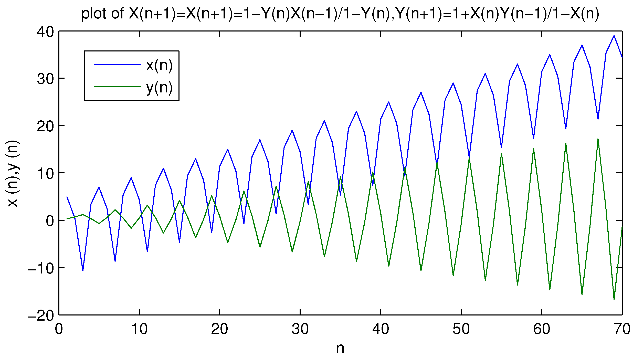
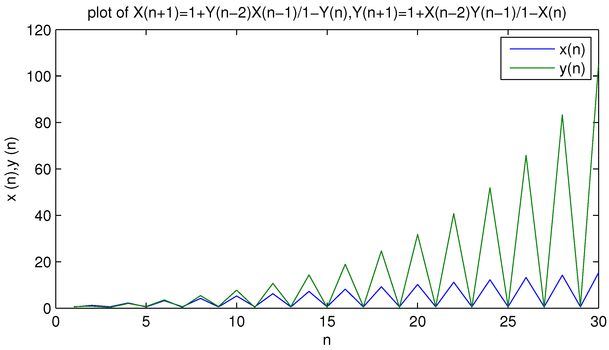
3. Numerical Examples

In this section, we present some numerical examples that support the above theoretical results.
Example 1.
Suppose System (1) under the initial conditions x 1 = 0.5 , x 0 = 2 , y 1 = 7 and y 0 = 0.8 . See Figure 1 below.
Example 2.
See Figure 2 below as an example for System (2) with the initial values x 1 = 5 , x 0 = 0.4 , y 1 = 0.3 , and y 0 = 0.7 .
Example 3.
Figure 3 below shows the behaviour of the solution of System (3) when the initial values x 2 = 0.5 , x 1 = 1.2 , x 0 = 0.6 , y 2 = 0.7 , y 1 = 0.8 , and y 0 = 0.3 .
Example 4.
Suppose the initial conditions for the system x n + 1 = 1 x n 1 y n 2 1 y n , y n + 1 = 1 y n 1 x n 2 1 x n are x 2 = 0.9 , x 1 = 1.2 , x 0 = 0.1 , y 2 = 0.3 , y 1 = 2 , and y 0 = 0.7 . See Figure 4.
Example 5.
Figure 5 shows the periodic nature of the solution of System (5) with the initial conditions x 2 = 0.4 , x 1 = 1 , x 0 = 0.6 , y 2 = 0.2 , y 1 = 3 , and y 0 = 0.8 .

4. Conclusions

In this paper, we obtained the expressions of the solutions of different classes of third-order rational systems of difference equations. In Section 1, the work of the authors on the same side of the difference equations, whether they are equations, systems of equations, or some applications of difference equations, is presented. After the introduction in Section 2, we have solved the first system of second order rational difference equations x n + 1 = 1 + x n 1 y n 1 y n , y n + 1 = 1 + y n 1 x n 1 x n . After finding the solutions, we provided numerical examples to illustrate the results. In Section 3, we obtained the form of the solution of the second system x n + 1 = 1 x n 1 y n 1 y n , y n + 1 = 1 + y n 1 x n 1 x n ; we also mentioned the solutions of the other systems x n + 1 = 1 + x n 1 y n 1 y n , y n + 1 = 1 y n 1 x n 1 x n , and x n + 1 = 1 x n 1 y n 1 y n , y n + 1 = 1 y n 1 x n 1 x n . Finally, Section 4 was devoted to the form of the solutions of the main system of third order fractional difference equations x n + 1 = 1 + x n 1 y n 2 1 y n , y n + 1 = 1 + y n 1 x n 2 1 x n and some other systems that we obtained the expressions of the solutions for and studied the periodicity nature of the solutions. Moreover, we confirmed our results using numerical simulations and drew them using Matlab program.

Author Contributions

Methodology, K.S.A.-B. and E.M.E.; Formal analysis, E.M.E.; Investigation, K.S.A.-B. and E.M.E.; Writing—original draft, K.S.A.-B.; Writing—review & editing, E.M.E. All authors have read and agreed to the published version of the manuscript.

Funding

This research work was funded by Institutional Fund Projects under grant no. (IFPIP: 283-130-1443).

Data Availability Statement

Not applicable.

Acknowledgments

This research work was funded by Institutional Fund Projects under grant no. (IFPIP: 283-130-1443). The authors gratefully acknowledge technical and financial support provided by the Ministry of Education and King Abdulaziz University, DSR, Jeddah, Saudi Arabia.

Conflicts of Interest

The authors declare no conflict of interest.

References

  1. El-Dessoky, M.M. On a solvable for some systems of rational difference equations. J. Nonlinear Sci. Appl. 2016, 9, 3744–3759. [Google Scholar] [CrossRef] [Green Version]
  2. Elsayed, E.M. Solution and attractivity for a rational recursive sequence. Dis. Dyn. Nat. Soc. 2011, 2011, 17. [Google Scholar] [CrossRef] [Green Version]
  3. Folly-Gbetoula, M.; Gocen, M.; Guneysu, M. General form of the solutions of some difference equations via Lie symmetry analysis. J. Anal. Appl. 2022, 20, 105–122. [Google Scholar]
  4. Ibrahim, T.F. Periodicity and analytic solution of a recursive sequence with numerical examples. J. Interdiscip. Math. 2009, 12, 701–708. [Google Scholar] [CrossRef]
  5. Ogul, B.; Simsek, D. On the recursive sequence, Dynamics of Continuous. Discret. Impuls. Syst. Ser. B Appl. Algorithms 2022, 29, 423–435. [Google Scholar]
  6. Touafek, N.; Elsayed, E.M. On the solutions of systems of rational difference equations. Math. Comput. Mod. 2012, 55, 1987–1997. [Google Scholar] [CrossRef]
  7. Das, S.E.; Bayram, M. On a system of rational difference equations. World Appl. Sci. J. 2010, 10, 1306–1312. [Google Scholar]
  8. Dilip, D.S.; Mathew, S.M. Dynamics of a second order nonlinear difference system with exponents. J. Egypt. Math. Soc. 2021, 29, 1–10. [Google Scholar] [CrossRef]
  9. Elabbasy, E.M.; Eleissawy, S.M. Asymptotic behavior of two dimensional rational system of difference equations. Dyn. Contin. Impuls. Syst. Ser. B Appl. Algorithms 2013, 20, 221–235. [Google Scholar]
  10. Elabbasy, E.M.; El-Metwally, H.; Elsayed, E.M. Global behavior of the solutions of difference equation. Adv. Differ. Equ. 2011, 2011, 1–16. [Google Scholar] [CrossRef] [Green Version]
  11. Kurbanli, A.S.; Cinar, C.; Yalcinkaya, I. On the behavior of positive solutions of the system of rational difference equations. Math. Comp. Mod. 2011, 53, 1261–1267. [Google Scholar] [CrossRef]
  12. Kurbanli, A.S. On the behavior of solutions of the system of rational difference equations xn+1 = xn−1/(ynxn−1 − 1), yn+1 = yn−1/(xnyn−1 − 1), zn+1 = 1/ynzn. World Appl. Sci. J. 2010, 10, 1344–1350. [Google Scholar]
  13. Cinar, C.; Yalcinkaya, I.; Karatas, R. On the positive solutions of the difference equation system xn+1 = m/yn, yn+1 = pyn/xn−1yn−1. J. Inst. Math. Comp. Sci. 2005, 18, 135–136. [Google Scholar]
  14. El-Metwally, H. Solutions form for some rational systems of difference equations. Dis. Dyn. Nat. Soc. 2013, 2013, 1–10. [Google Scholar] [CrossRef] [Green Version]
  15. Kara, M.; Yazlik, Y. On the solutions of three-dimensional system of difference equations via recursive relations of order two and applications. J. Appl. Anal. Comput. 2022, 12, 736–753. [Google Scholar] [CrossRef]
  16. Mansour, M.; El-Dessoky, M.M.; Elsayed, E.M. The form of the solutions and periodicity of some systems of difference equations. Dis. Dyn. Nat. Soc. 2012, 2012, 1–17. [Google Scholar] [CrossRef] [Green Version]
  17. Ozban, A.Y. On the system of rational difference equations xn = a/yn−3, yn = byn−3/xn−qyn−q. Appl. Math. Comp. 2007, 188, 833–837. [Google Scholar] [CrossRef]
  18. Sroysang, B. Dynamics of a system of rational higher-order difference equation. Dis. Dyn. Nat. Soc. 2013, 2013, 1–5. [Google Scholar] [CrossRef]
  19. Touafek, N.; Elsayed, E.M. On the periodicity of some systems of nonlinear difference equations. Bull. Math. Soc. Sci. Math. Roum. 2012, 55, 217–224. [Google Scholar]
  20. Yalcinkaya, I. On the global asymptotic behavior of a system of two nonlinear difference equations. ARS Comb. 2010, 95, 151–159. [Google Scholar]
  21. Zhang, Y.; Yang, X.; Megson, G.M.; Evans, D.J. On the system of rational difference equations. Appl. Math. Comp. 2006, 176, 403–408. [Google Scholar] [CrossRef]
  22. Zhang, Q.; Yang, L.; Liu, J. Dynamics of a system of rational third order difference equation. Adv. Differ. Equ. 2012, 2012, 1–6. [Google Scholar] [CrossRef] [Green Version]
  23. Elsayed, E.M.; Din, Q.; Bukhary, N.A. Theoretical and numerical analysis of solutions of some systems of nonlinear difference equations. AIMS Math. 2022, 7, 15532–15549. [Google Scholar] [CrossRef]
  24. Elsayed, E.M. Solutions of rational difference system of order two. Math. Comput. Mod. 2012, 55, 378–384. [Google Scholar] [CrossRef]
  25. Elsayed, E.M.; Alharbi, K.N. The expressions and behavior of solutions for nonlinear systems of rational difference equations. J. Innov. Appl. Math. Comput. Sci. (JIAMCS) 2022, 2, 78–91. [Google Scholar]
  26. Karatas, R.; Gelisken, A. A Solution Form of A Higher Order Difference Equation. Konuralp J. Math. 2021, 9, 316–323. [Google Scholar]
  27. Taskara, N.; Buyuk, H. On The Solutions of Three-Dimensional Difference Equation Systems Via Pell Numbers. Eur. J. Sci. Technol. 2022, 34, 433–440. [Google Scholar] [CrossRef]
  28. Berkal, M.; Abo-Zeid, R. On a Rational (P+1)th Order Difference Equation with Quadratic Term. Univers. J. Math. And Appl. 2022, 5, 136–144. [Google Scholar] [CrossRef]
  29. El-Moneam, M.A. On the Global of the Difference Equation. Commun. Adv. Math. Sci. 2022, 5, 189–198. [Google Scholar]
  30. Kara, M. Solvability of a Three-Dimensional System of Nonlinear Difference Equations. Math. Sci. Appl. E-Notes 2022, 10, 1–15. [Google Scholar] [CrossRef]
  31. Aljoufia, L.S.; Ahmeda, A.M.; Al Mohammadya, S. Global behavior of a third-order rational difference equation. J. Math. And Computer Sci. 2022, 25, 296–302. [Google Scholar] [CrossRef]
  32. Alotaibi, A.M.; El-Moneam, M.A. On the dynamics of the nonlinear rational difference equation xn+1 = (αxn−m + δxn)(β + γxn−kxn−l(xn−k + xn−l)). AIMS Math. 2022, 7, 7374–7384. [Google Scholar] [CrossRef]
  33. Beverton, R.J.; Holt, S.J. On the Dynamics of Exploited Fish Populations; Fish Invest: London, UK, 1957; p. 19. [Google Scholar]
  34. Khaliq, A.; Ibrahim, T.F.; Alotaibi, A.M.; Shoaib, M.; El-Moneam, M. Dynamical Analysis of Discrete-Time Two-Predators One-Prey Lotka–Volterra Model. Mathematics 2022, 10, 4015. [Google Scholar] [CrossRef]
  35. Din, Q.; Elsayed, E.M. Stability analysis of a discrete ecological model. Comput. Ecol. Softw. 2014, 4, 89–103. [Google Scholar]
  36. Khan, A.Q.; Tasneem, M.; Younis, B.; Ibrahim, T.F. Dynamical analysis of a discrete-time COVID-19 epidemic model. Math. Meth. Appl. Sci. 2022, 46, 4789–4814. [Google Scholar] [CrossRef]
  37. Al-Khedhairi, A.; Elsadany, A.A.; Elsonbaty, A. On the dynamics of a discrete fractional-order cournot–bertrand competition duopoly game. Math. Probl. Eng. 2022, 2022, 8249215. [Google Scholar] [CrossRef]
  38. Ibrahim, T.F. Asymptotic behavior of a difference equation model in exponential form. Math. Methods Appl. Sci. 2022, 45, 10736–10748. [Google Scholar] [CrossRef]
  39. Khaliq, A.; Mustafa, I.; Ibrahim, T.F.; Osman, W.M.; Al-Sinan, B.R.; Dawood, A.A.; Juma, M.Y. Stability and Bifurcation Analysis of Fifth-Order Nonlinear Fractional Difference Equation. Fractal Fract. 2023, 7, 113. [Google Scholar] [CrossRef]
Figure 1. Represents behavior of System (1) when x 1 = 0.5 , x 0 = 2 , y 1 = 7 and y 0 = 0.8 .
Mathematics 11 01047 g001
Figure 2. Shows the behavior for System (2) with the initial values x 1 = 5 , x 0 = 0.4 , y 1 = 0.3 and y 0 = 0.7 .
Mathematics 11 01047 g002
Figure 3. Expresses the solution of System (3) when the initial values x 2 = 0.5 , x 1 = 1.2 , x 0 = 0.6 , y 2 = 0.7 , y 1 = 0.8 and y 0 = 0.3 .
Mathematics 11 01047 g003
Figure 4. Plot of solutions of System (4) when the initial conditions are x 2 = 0.9 , x 1 = 1.2 , x 0 = 0.1 , y 2 = 0.3 , y 1 = 2 and y 0 = 0.7 .
Mathematics 11 01047 g004
Figure 5. Shows the periodicity of the solution of System (5) with x 2 = 0.4 , x 1 = 1 , x 0 = 0.6 , y 2 = 0.2 , y 1 = 3 and y 0 = 0.8 .
Mathematics 11 01047 g005
Disclaimer/Publisher’s Note: The statements, opinions and data contained in all publications are solely those of the individual author(s) and contributor(s) and not of MDPI and/or the editor(s). MDPI and/or the editor(s) disclaim responsibility for any injury to people or property resulting from any ideas, methods, instructions or products referred to in the content.

