Article

Training Multilayer Neural Network Based on Optimal Control Theory for Limited Computational Resources

by
Ali Najem Alkawaz
1,
Jeevan Kanesan
1,*,
Anis Salwa Mohd Khairuddin
1,
Irfan Anjum Badruddin
2,*,
Sarfaraz Kamangar
2,
Mohamed Hussien
3,4,
Maughal Ahmed Ali Baig
5 and
N. Ameer Ahammad
6
1
Department of Electrical Engineering, Faculty of Engineering, Universiti Malaya, Kuala Lumpur 50603, Malaysia
2
Mechanical Engineering Department, College of Engineering, King Khalid University, Abha 61421, Saudi Arabia
3
Department of Chemistry, Faculty of Science, King Khalid University, P.O. Box 9004, Abha 61413, Saudi Arabia
4
Pesticide Formulation Department, Central Agricultural Pesticide Laboratory, Agricultural Research Center, Dokki, Giza 12618, Egypt
5
Department of Mechanical Engineering, CMR Technical Campus, Kandlakoya, Medchal Road, Hyderabad 501401, India
6
Department of Mathematics, Faculty of Science, University of Tabuk, Tabuk 71491, Saudi Arabia
*
Authors to whom correspondence should be addressed.
Mathematics 2023, 11(3), 778; https://doi.org/10.3390/math11030778
Submission received: 30 December 2022 / Revised: 23 January 2023 / Accepted: 27 January 2023 / Published: 3 February 2023
(This article belongs to the Special Issue Mathematical Problems in Mechanical Engineering, 2nd Edition)

Abstract

:
Backpropagation (BP)-based gradient descent is the general approach to train a neural network with a multilayer perceptron. However, BP is inherently slow in learning, and it sometimes traps at local minima, mainly due to a constant learning rate. This pre-fixed learning rate regularly leads the BP network towards an unsuccessful stochastic steepest descent. Therefore, to overcome the limitation of BP, this work addresses an improved method of training the neural network based on optimal control (OC) theory. State equations in optimal control represent the BP neural network’s weights and biases. Meanwhile, the learning rate is treated as the input control that adapts during the neural training process. The effectiveness of the proposed algorithm is evaluated on several logic gates models such as XOR, AND, and OR, as well as the full adder model. Simulation results demonstrate that the proposed algorithm outperforms the conventional method in terms of improved accuracy in output with a shorter time in training. The training via OC also reduces the local minima trap. The proposed algorithm is almost 40% faster than the steepest descent method, with a marginally improved accuracy of approximately 60%. Consequently, the proposed algorithm is suitable to be applied on devices with limited computation resources, since the proposed algorithm is less complex, thus lowering the circuit’s power consumption.

1. Introduction

Multilayer neural networks (MLNNs) effectively impact various applications, such as computer vision, robotics, image classification or prediction, etc. The standard artificial neural networks include learning factors, computing, intelligent signal processing, and machine learning (ML) [1,2]. Various techniques have been proposed for a nonlinear algorithm for optimization and learning problems to overcome the limitations of linear computation [3,4]. Furthermore, training MLNNs is essential to verify various parameters, such as several inputs and hidden layers, output layers, types of activation functions, training rules, etc. It is necessary to consider a MLNN in two phases: training and prediction. In both phases, the number of inputs, hidden layers, and output layers must be the same. The most widely used method of training MLNNs is the backpropagation algorithm (BP), which depends on stochastic gradient decent (SGD). The term “train” refers to the steps of the neural network process that consist of feedforward and backward passes [5,6]. Additionally, the loss function is used in a forwarding pass to evaluate the prediction outputs. The chain rule is employed in the back pass to compute the gradient using trainable parameters (weights and biases) [7,8]. Meanwhile, optimization using the optimal control (OC) problem in nonlinear systems is widely researched, mainly in the design of control systems. The challenge of OC problems in nonlinear systems is its inherently nonlinear nature, whereby the nonlinear OC problem cannot be solved analytically [9,10]. Previous researchers have discussed and concentrated on the hypothesis of control theory for synthesis and evaluation training algorithms to overcome the OC’s limitations. For instance, Li and Hao [11] proposed an alternative theoretical and algorithmic basis for deep learning that may apply to many contexts based on a discrete-time OC viewpoint of deep learning by utilizing Pontryagin’s Minimum Principle (PMP) and the method of successive approximation (MSA). Chen and Pung [12] studied the convergence rate analysis by optimizing hidden neurons in distinct layers instead of choosing a random number that arbitrarily produces various clusters of hidden parameters and then finding the best number that obtained a small error. Bang bang OC has been developed to find the optimal step size in each epoch to solve the slow convergence rate of BP [7]. However, this study does not show the OC viewpoint, such as states, co-states, and function input. According to neural networks, the numerical system of fractional optimal control problems (FOCPs) has been discussed in [13] by applying trial solutions for the state, co-state, and function control; meanwhile, the results are constructed merely on two-layer perceptron to reduce the error function. Plakias and Boutalis [14] proposed a novel fusion neural architecture based on Lyapunov’s nonlinear online dynamic system. An ordinary differential equations (ODE) solver is more suitable for solving nonlinear systems [15]. The neural system is combined with the suggested update rule of neural weights to achieve the fast convergence of the identification processes by utilizing a discretization of a continuous-time dynamic system [16]. Wen et al. [17] suggested a fuzzy logic control to adjust the neural network’s learning factor dynamically. Adaptive learning rate clipping (ALRC) was developed to restrict BP losses to several standard deviations [18]. Designing logic gate circuits is proposed in [19,20] by using a multilayer neural network to train and test models. The results show that the multilayer perceptron has a higher velocity and minor delay. A full adder (FA) model was designed with two types of sigmoid neural network functions. The model was implemented on FPGA and compared with the theoretical value. Kaya [21] proposed a new training neural network, named a hybrid artificial bee colony, based on an effective scout bee stage. Arithmetic crossover was employed in the solution generation structures of the employed bee and onlooker bee stages. The execution of the proposed technique was evaluated on the solution of global optimization problems. Empirical results illustrated the proposed algorithm had better performance in terms of convergence speed and solution quality. Mahmood et al. [22] suggested a new design of an intelligent Bayesian regularization backpropagation neural network based on a stochastics numerical framework in order to investigate the dynamic motion of a third-grade fluid in the planner channel using MLNN with efficient Bayesian optimization. Soon et al. [23] proposed a classification system based on a principal component analysis convolutional network (PCN), in which convolutional filters were used to extract discriminative and hierarchical features. According to the experimental results, the proposed PCN system is feasible for real-time applications because of its robustness against various challenging distortions such as translations, rotations, illumination conditions, and noise contaminations. In general, optimal control is a set of mathematical expressions including the objective function and all the constraints, known as the optimization problem. The constraints include the state equation, any conditions that must be satisfied at the beginning and at the end of the time horizon, and any constraints that restrict choices between the beginning and the end. At a minimum, dynamic optimization problems must include the objective function, the state equation (s), and the initial conditions for the state variables. The application of a backtracking search algorithm (BSA) on fed-batch fermentation processes was proposed by [24]. Nevertheless, all the case studies presented in this paper consisted of single objective problems. It is interesting to evaluate the performance of metaheuristics in solving multi-objectives fed-batch fermentation problems. Therefore, the problem that is being addressed in this work is to reduce the mean quantization error of SOM by formulating a conventional self-organizing map algorithm as the optimal control problem. The mean quantization error equation becomes the objective function to be minimized, and the online mode weight updating equation becomes the state equation. Jeevan et al. [25] carried out a genetic algorithm (GA) to determine the optimal chip placement of a multi-chip model (MCM) and printed circuit board (PCB) under certain thermal constraints. The comparison results of optimal placement utilizing GA with other placement techniques were elaborated. However, the evaluation was valid under steady-state conditions and for MCM or PCB constant characteristics. The chip/component can only be a specific standard size. Furthermore, Hoo et al. [26] developed a Variable Order Ant System (VOAS) to optimize the area and wirelength by combining VOAS with a floorplan model called Corner List (CL). Two classes of ants were introduced to determine the local information in this study. The results showed that the VOAS had better improvement in terms of pure area optimization and the composite function of area and wirelength compared to other benchmark techniques. In terms of the new design of a power amplifier (PA) for next-generation wireless communication, the researchers in [27] suggested a new approach to enhance the performance of PAs in the context of efficiency and linearity. The aim was to eliminate design cost and space on board. Further, Mallick [28] tried to determine the effect of two classes of grass-trimming machine engine noise on the operator in a natural working environment. Experimental results showed that the sound pressure level of the grass-trimmer machine engine was higher than the limit of noise recommended by other machine engines for approximately 98 h weekly. Hoo [29] proposed a Hierarchical Congregated Ant System (H-CAS) to perform a variable order bottom-up hierarchical placer that could generate compact placement in a chip layout for hard and soft modules of floor planning. Empirical outcomes demonstrated that the H-CAS performed more efficiently as a placer than a state-of-the-art technique in terms of circuit size, complexity increase, stability, and scalability. Additionally, the H-CAS excelled in all other techniques for higher-size issues in area minimization.
By analyzing the literature reported above, it can be concluded that there are many existing works for training MLNNs that employ a conventional method based on analytical and gradient descent techniques. Nevertheless, minimizing error function with less computational time by formulating the parameters of MLNNs has more challenges. To the authors’ knowledge, this aspect has not been previously covered in the literature. Thus, this paper proposes a new method to train a neural network using OC by formulating the weights and biases parameters as state equations and the learning rate as the input control to minimize error function with less computation time. The main contribution of this paper is to propose a new multilayer neural network training algorithm based on OC theory by modeling adaptable parameters as state equations, as well as the learning rate as an input control with the necessary conditions. The weights and biases are the updating parameters used to develop the Hamiltonian equation and to solve the state, co-state, and stationary equations. The parameters satisfy the necessary condition based on Hamiltonian and switch control that find the optimal input at each time. A logic gates model and full adder are introduced to assess the proposed approach. Furthermore, simulation results validate that the proposed training algorithm outperforms the typical training approach regarding speed, time, and ability to escape from local minima. As a result, it takes up less physical space and is less complex, lowering the circuit’s power consumption.
The remaining sections of this paper are structured as follows: Section 2 introduces backpropagation and learning training topology. Section 3 presents an optimal control theory and discrete-time Pontryagin’s Minimum Principle and logic gate circuit. The simulation results and a discussion are given in Section 4. Finally, the conclusion is provided in Section 5.

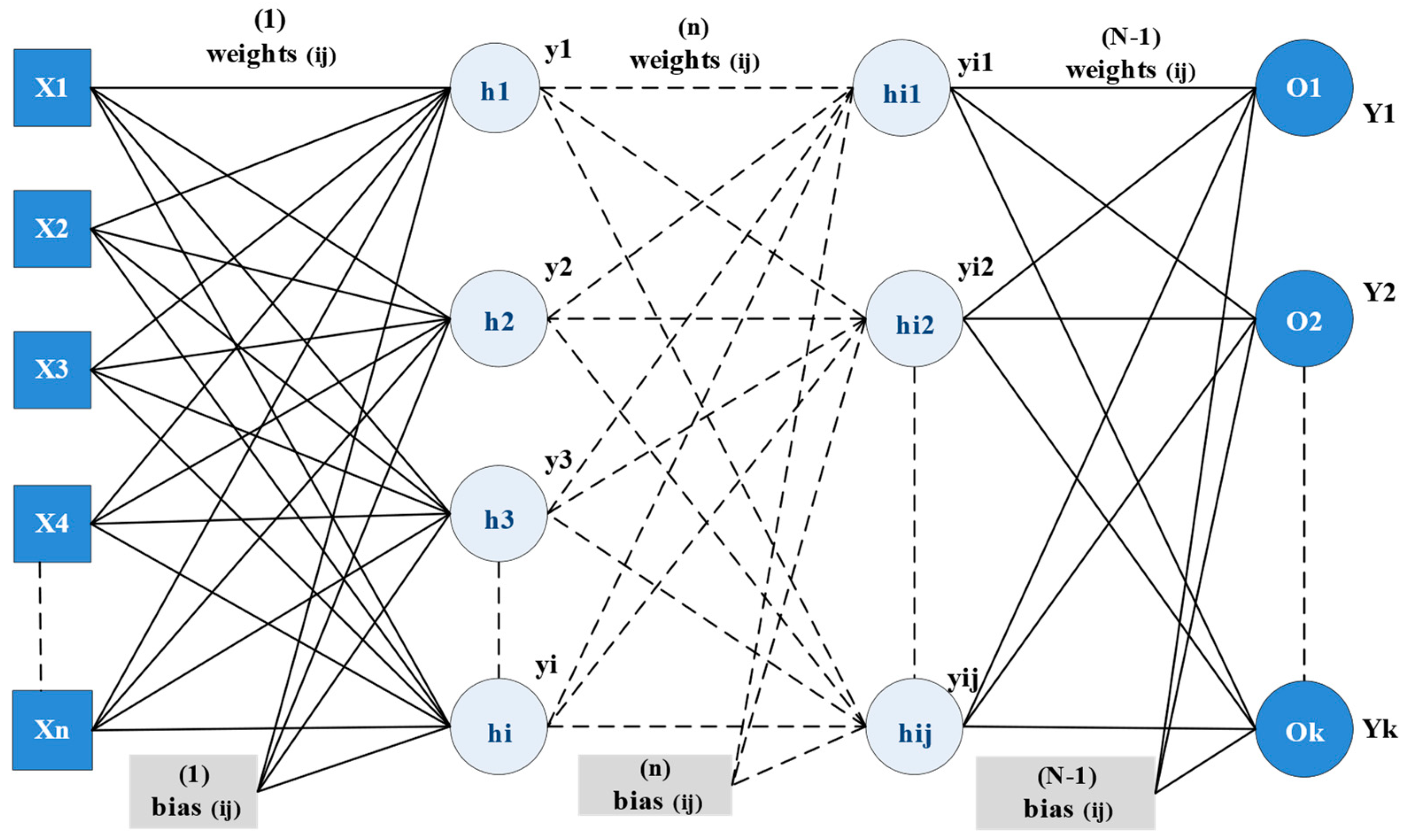
2. Backpropagation Learning Topology

The highly fundamental approach to the training MLNN is the BP developed by Rumelhart et al. [5,30]. Generally, a BP comprises three layers. The input layer is where the data is provided to the network. Hidden layers might consist of one or more layers where data are handled. The output layer carries out the outcomes of the given data input [31,32,33]. BP is a suitable and uncomplicated iterative process that normally works well with complex data, unlike other learning techniques such as the Bayesian technique, with adequate computational properties with large-scale data [34]. Furthermore, the BP algorithm is utilized for training a neural network by changing the parameters (weights and biases) of each neuron. However, the essential goal of the training is to reduce the discrepancy between the desired data input and output samples, which is called the loss function, such as the Mean Square Error (MSE) via a gradient descent algorithm, which is dependent on the error rate obtained in the previous epochs (i.e., iteration). However, the MSE is given as follows [35]:
M S E ( d , y ) = 1 n i = 1 n ( Y i d i ) 2
where n denotes the entire number of data inputs, d i corresponds to the desired dataset, and Y i represents actual output samples from the output layer of the MLNN. Suppose a simple MLNN model as illustrated in Figure 1 with an input layer X 1 ,   X 2 ,   X 3 ,   X 4 ,     X N , hidden layer H 1 ,   H 2 ,   H 3 ,     H N , and output layer Y 1 ,   Y 2 ,   Y 3 ,     Y N , and the connections between each layer are the weights and biases vectors. The outputs for each unit in each layer are obtained to utilize the output for the whole neural network based on the forward propagate rule that is defined as follows:
Z = i = 1 n θ i j X i ( k )
Here, θ i j denotes a weight matrix that links neurons i in the input layers with neurons j in the hidden layer, as well as between hidden j and output y layers. X i represents the input layer vector for the i neuron, n represents several neurons, and k is the pattern. Each iteration (epoch) will be fed into the network, and each output will be evaluated individually.
However, if the network has a bias in the neurons, the formula is given as follows:
Z = i = 1 n [ θ i j X i ( k ) ] + b i j
An activation function (Sigmoid, Tanh, Linear, ReLU) is selected to find the output from each layer. The sigmoid activation function is used in this work because it exists between (0, 1) and the smooth gradient value. Hence, it is proper for a shallow network, especially for models in which the probability is predicted as an output, which is given as follows [36]:
σ ( Z ) = 1 1 + e x p Z
The output function of each layer after applying the sigmoid function would be computed as follows:
Y i ( t ) = 1 1 + e x p [ i = 1 n [ θ i j X i ( k ) ] + b i j ]
The loss function formulation MSE, as mentioned in Equation (1), is applied to compute the error between the desired and actual outputs. To minimize error, the BP algorithm based on stochastic gradient descent is used to update the weights and biases in the k + 1 th iteration via the following form:
[ θ K + 1 = θ K η D K b K + 1 = b K η D K ]
where η is the learning factor. The step size is highly influential on the convergence rate. θ K ,   b K denote the weights and biases parameter vectors of the previous iteration, respectively, and D K indicates the gradient vector, which is given as follows:
[ D K = L θ i j D K = L b i j ]
In Equation (7), L indicates the loss function MSE of the outputs in the k th step of the training operation. Alternatively, in each iteration, the weights and biases are updated, where the L θ i j and L b i j terms are the derivation of the MSE error for each trainable parameter θ i j , b i j vectors. Meanwhile, the derivation of the loss function of all trainable parameters can be obtained using the chain rule, particularly with a more hidden layer network. Thus, each iteration’s parameters are updated, and the error function is evaluated consequently [30]. The entire procedure of the BP is given in Algorithm 1.
Algorithm 1: Process of BP algorithm
1. procedure Backpropagation ( D ,   η ).
2. input: D = [ ( X K ,   Y K ) ] K = 1 n , η = learning factor.
3. randomly initialize all weights and biases.
4.    repeat.
5.      for all ( X ( i ) , Y ( i ) ) ∈ D do
6.         compute Y j ( i ) according to the current parameter.
7.         compute D K
8.         update θ i j , b i j via gradient descent method.
9.      end for.
10.    until achieve some criterion is satisfied.
11. end procedure.

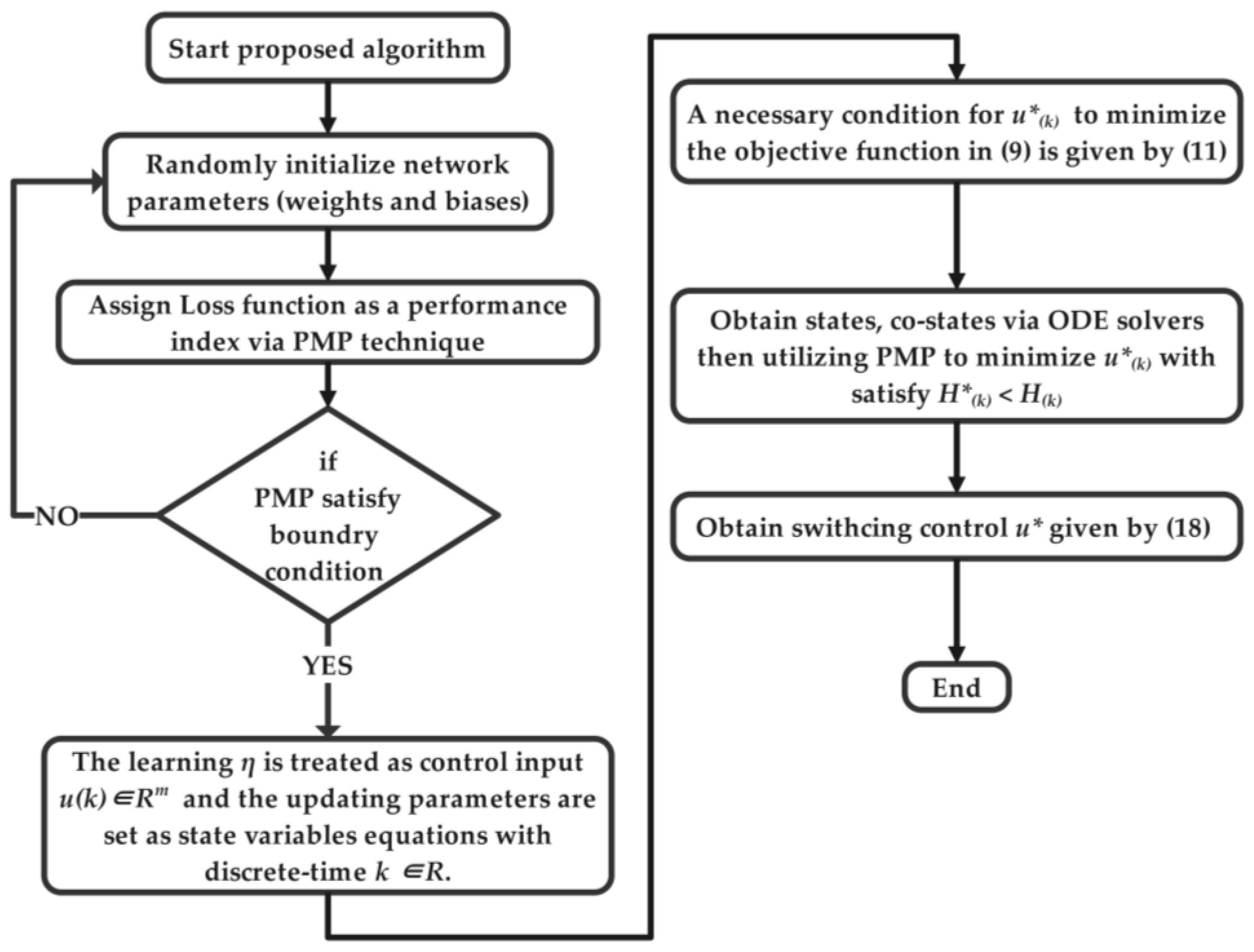
3. Optimal Control Theory

In the 1950s, dynamic programming with Hamiltonian partial differential equations and the Pontryagin Minimum Principle (PMP) were used to produce optimal control. The calculus of variations provides a generalization of Euler Lagrange equations [37]. Furthermore, training MLNNs is formalized using OC theory. Let H     Z + indicate the number of layers and [ X   s , 0   R d o   : s = 0 , , S ] denote a collection of sample inputs (time series). Here, S Z + is considered as a sample size [38,39]. Assume the deterministic dynamic system equation given as:
X k + 1 = f t ( X s , k , θ k ) ,           k = 0 , 1 , T 1
where each k ,   f k   : R d t × θ k   R d t + 1 is a transformation on the state. For instance, in original MLNNs, this can characterize a trainable affine transformation or nonlinear function [15]. As mentioned in Section 2, the aim of training MLNNs via BP on a descent gradient algorithm is to adjust all parameters θ : = [ θ k   : k = 0 , T 1 ] , and hence to minimize the loss function MSE. Hence, to train MLNNs using the OC technique, the MSE function given in Equation (1) is used as a performance index via PMP, which will be deliberated in the following subsection. Moreover, the flowchart in Figure 2 illustrates the steps of the proposed algorithm, in which PMP provides a necessary condition for optimality that must satisfy a boundary condition to obtain the OC law performance using the Pontryagin Hamiltonian function. The learning factor (step size) η is treated as the control input u ( k ) m , and the updating parameters θ k , b k , , which are given in Equation (6), are set as state variable equations with discrete-time k . Therefore, the performance index and state variables are presented as:
M i n       J = t 0 t f 1 n i = 1 n ( Y i d i ) 2   d t  
Subject   to :   [ θ ˙ i j = u     L θ i j b ˙ i j = u     L b i j ]

3.1. Pontryagin Minimum Principle

A necessary condition for the OC in Equation (9) is known as the PMP, which was developed by Boltyanskii et al., 1960 and Pontryagin, 1987. The necessary optimality conditions are utilized in the form of the minimization of a specific Hamiltonian function. The Hamiltonian H : [ 0 ,   T ] is given as follows:
H k ( x ( k ) ,   u ( k ) ,   λ ( k ) , k ) f 0 ( x ( k ) ,   u ( k ) , k ) + [ λ ( k ) ] T S ( x ( k ) ,   u ( k ) , k )
where x ( k ) ,   λ ( k )   n are the state and co-state vectors of the system, respectively, and u ( k ) m is the input of the state space system, k . The optimal parameters’ state, co-state, and control function are denoted by x ( k ) , λ ( k ) , and u ( k ) respectively. Hence, a necessary condition for u ( k ) to minimize the objective function in Equation (9) is given for all k [ t 0 ,   t f ] as well as all admissible controls as follows:
H k ( x ( k ) , λ ( k ) ,   u ( k ) , k )     H k ( x ( k ) ,   λ ( k ) , u ( k ) , k )
Equation (11) indicates that the OC must minimize the Hamiltonian function using PMP, which shows the optimal values of states, co-states, and input control x ( k ) , λ ( k ) , u ( k ) . It should then satisfy the following conditions:
{ H ( x ( k ) ,   u ( k ) ,   λ ( k ) , k ) x = λ ˙ ( k ) H ( x ( k ) ,   u ( k ) ,   λ ( k ) , k ) λ = X ˙ ( k ) H ( x ( k ) ,   u ( k ) ,   λ ( k ) , k ) u = 0
Functions f 0   and   S denote the performance index and state equations, as illustrated in Equation (10), substituted into the Hamiltonian Equation (12), which gives a system of an ordinary differential equation (ODE) that can be offered using numerical methods or an alternative approach. Furthermore, the conditions in Equation (12) present a straightforward ODE system that can quickly obtain the solution. The summary of minimizing the MSE using the OC based on PMP is expressed in Algorithm 2.
Algorithm 2: Optimal control based on PMP algorithm
1. system optimal control ( D ,   u ,   P I ).
2. input: D = [ ( X K ,   Y K ) ] K = 1 n , u = input control, P I = performance index.
3. randomly initialize θ i j and b i j .
4. set optimal parameters.
5.    repeat.
6.      for all ( X ( i ) , Y ( i ) ) ∈ D do
7.        define the Hamiltonian H k : [ 0 ,   T ] .
8.        evaluate necessary optimality conditions.
9.        obtain states, co-states via ODE solvers.
10.         utilizing PMP to minimize u ( k ) with satisfy H ( k ) < H ( k ) .
11.      end for.
12.     until criteria are satisfied.
13.  end procedure.

3.2. Problem Formulation

This section includes an evaluation of the control vector u k , which is modeled as the learning rate to minimize the error objective function, as mentioned in Equation (9), with a specific value of the maximum iteration ( t m a x ) utilizing PMP to satisfy the Hamiltonian equation. A general MLNN model with a sigmoid activation function that includes an input layer, hidden layers, and an output layer is illustrated in Figure 3, in order to find the explicit ODE for states, costate variables, and model parameters.
Based on the gradient descent method [40], the state variables of the general model can be evaluated as:
θ ˙ 11 = u L ( 1 ) θ 11 b ˙ 11 = u L ( 1 ) b 11 θ ˙ 12 = u L ( 2 ) θ 12 b ˙ 12 = u L ( 2 ) b 12 · , · · · θ ˙ i j = u L ( n ) θ i j b ˙ i j = u L ( n ) b i j
where L denotes the loss function MSE. The terms of the derivation loss function need to be found for the vectors of each trainable parameter θ i j   , b i j by applying the chin rule starting from the last layer and towards the entire network with the required parameters θ i j   , b i j until the first layer. Thus, the following equation can be obtained:
L ( n ) θ i j = L ( n ) Y k · Y k o k · o k y i j · y i j h i j · h i j y i · y i h i · h i θ i j L ( n ) b i j = L ( n ) Y k · Y k o k · o k y i j · y i j h i j · h i j y i · y i h i · h i b i j
To apply the OC with a particular discretized time horizon and to minimize the loss function considered in Equation (9), it is necessary to obtain the Hamiltonian equation rewritten as follows:
{ H = 1 n i = 1 n ( Y i d i ) 2 + [ λ k ] T   [ θ ˙ i j = u     L ( n ) θ i j b ˙ i j = u     L ( n ) b i j ]     H = 1 n i = 1 n ( Y i d i ) 2 u ( λ 1 L ( n ) θ i j + λ 2 L ( n ) b i j )         , k = 1 , 2 , n
The necessary conditions for optimality are expressed as:
H θ ( k ) , u ( k ) , λ ( k ) , k θ i j = θ i j 1 n i = 1 n Y i d i 2 + θ i j u λ 1 L ( n ) θ i j + λ 2 L ( n ) b i j = λ ˙ 1 H θ ( k ) , u ( k ) , λ ( k ) , k b i j = b i j 1 n i = 1 n Y i d i 2 + b i j u λ 1 L ( n ) θ i j + λ 2 L ( n ) b i j = λ ˙ 2 H θ ( k ) , u ( k ) , λ ( k ) , k λ 1 = u L ( n ) θ i j = θ ˙ i j H θ ( k ) , u ( k ) , λ ( k ) , k λ 2 = u L ( n ) b i j = b ˙ i j H θ ( k ) , u ( k ) , λ ( k ) , k u = λ 1 L ( n ) θ i j λ 2 L ( n ) b i j = 0
The minimization principle indicates that the OC input u ( k ) ought to satisfy H ( k ) < H ( k ) , which implies that:
1 n i = 1 n ( Y i d i ) 2 u ( λ 1 L ( n ) θ i j + λ 2 L ( n ) b i j ) < 1 n i = 1 n ( Y i d i ) 2 u ( λ 1 L ( n ) θ i j + λ 2 L ( n ) b i j )
Equation (17) concludes with a switching control, which is given depending on the value of H u that is computed from Equation (16). However, the switching control is provided by:
{ u = u m i n , if     H u > 0 u = u m a x , if     H u < 0

3.3. Logic Gate and Full Adder

In this section, logic gates pattern models are used (OR, XOR, AND, NAND, NOR, and XNOR), e.g., gates with two inputs and one output, as shown in Table 1. This includes a four-bit ripple carry full adder (FA), including one OR, two XOR, and two AND gates to evaluate the proposed training.
Moreover, FA includes three inputs and two outputs as depicted in Figure 4; however, two input data bits are utilized first, and the third input is used as a carrying bit. On the other hand, the output carries a bit on the FA circuit, transfers the carry bit to the next FA, and it achieves the addition by considering three input values. The logic circuit and truth table of the FA are portrayed in Figure 5. The neural network used in this model with one hidden layer has two neurons.
Then, the Boolean expression for a FA is given as follows:
( S U M = ( A B ) C i n C o u t = A . B + C i n ( A B ) )
In training a four-bit FA, the optimal training parameters of the logic gates that are combined are taken to generate a FA circuit to calculate the sum (SUM) and (CARRY-OUT). It is then compared with the Boolean expression mentioned in Equation (19) as well as the standard algorithm.

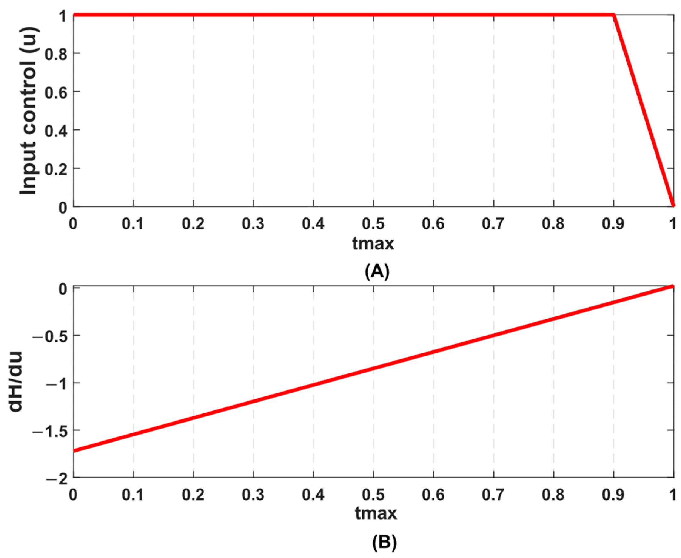
4. Results and Discussion

The training of MLNNs using two conventional BP methods with certain step size values and several iterations for each epoch and the proposed OC with minimum time and minimum loss function is discussed in this section. Moreover, training logic gates such as the XOR gate and four-bit FA using typical and proposed training approaches are proposed. In addition, the values of the weights and biases have been chosen randomly. For the proposed training method, the ODE15’s function is utilized to obtain the values of the states and co-states, respectively. In addition, numerical comparisons between the results of the two approaches are introduced. Since the proposed approach has better results in terms of the shorter time of training by reducing the local minima trap, as well as improved accuracy with less errors compared to the conventional method, the benefits of the proposed method could be suitably applied on devices with limited computational resources, since the proposed algorithm is less complex, thus lowering the circuit’s power consumption. The simulation result of the MSE of the XOR model is shown in Figure 6. Experimental results were conducted using MATLAB 2022B, Intel(R) Core™ i7-8565U CPU @ 1.8GHZ.
Figure 6 illustrates that the MSE using the standard BP method after 37294 epochs is 2.563 × 10⁻⁶, whereas the proposed results of the OC training method with t m a x = 1 , discretization = 0.1, and M a x _ i t e r = 2 are equal to 5.679 × 10⁻¹⁰. In addition, the simulation time of the proposed method needs only 2.31 s. In contrast, BP takes more than 4.16 s. This indicates that the proposed OC-based training is much faster towards the convergence of local minima than BP training. Meanwhile, the proposed training approach is more adaptive and robust in training MLNNs. The states and co-states of the system have been solved using the hybrid Runge–Kutta order 1 and 5, as demonstrated in Figure 7, and the input control u with a switching function H u of the proposed method are exhibited in Figure 8. In addition, switching control is obtained based on the optimality condition value mentioned in Equation (18). Table 2 shows that the proposed training approach is more rapid than the BP neural network’s final outputs and training time. Thus, it is suitably utilized on limited computational devices, since the proposed algorithm is less complex, and hence lowers the power consumption circuit.
As mentioned in Section 3.3, the FA has three inputs (A, B, C in ), and the sum with carrying is represented as an output, using Boolean expression as a typical technique to obtain the full adder’s output. However, two different methods are used to achieve the output by reducing the power consumption of the circuit. Some logic gates with training parameters based on the logic circuit of the FA are used. Hence, XOR, AND, and OR trainable parameters are used for conventional and OC training, and feedforward propagation is used to find the outputs. The comparison results are presented in Table 3. Often, in the case of a design circuit that includes 4-, 8-, 16-, 32-bit, and N-bit FA, it is necessary to repeat the whole operation, and each carryout of a FA will be input to the next FA.

5. Conclusions

This paper proposed a new approach in training MLNNs. In particular, a solution of OC theory based on PMP has been presented to train a neural network with discrete-time optimal control viewpoints of the MLNNs’ differentiable functions (states, co-states, and input control). In other words, the proposed training method is a more accurate solution than the conventional BP method, which depends on a gradient descent algorithm to reduce the loss function MSE. The output and computation time are superior to the BP algorithm. Furthermore, the theoretical results have been validated by numerical simulations to demonstrate the efficiency of the proposed method. Different logic models (XOR, AND, NAND, etc.) and FA models are presented to evaluate the proposed method. The proposed training algorithm performs well in speed and ability to escape from local minima, with approximately 40% faster time than the steep decent technique and a marginally improved accuracy of almost 60%. Hence, it is suitable to be applied on devices with limited computational resources, since the proposed algorithm is less complex, thus lowering the circuit’s power consumption. Further study with a different application with huge parameters, e.g., UCI datasets, can be employed to evaluate the effectiveness of the proposed algorithm. Moreover, we can utilize more hidden layers, more training points, and also heuristic algorithms in the optimization step, such as the genetic algorithm and particle swarm optimization, or other existing unconstrained optimization techniques could be another option.

Author Contributions

Conceptualization, A.N.A., J.K. and A.S.M.K.; methodology, A.N.A., J.K. and I.A.B.; software, S.K., M.H., M.A.A.B. and N.A.A.; validation, A.N.A., J.K., A.S.M.K. and I.A.B.; formal analysis, S.K., M.H., M.A.A.B. and N.A.A.; investigation, J.K., A.S.M.K. and A.N.A.; resources, S.K., M.H., M.A.A.B. and N.A.A.; data curation, A.N.A., J.K., A.S.M.K. and I.A.B.; writing—original draft preparation, A.N.A., J.K. and A.S.M.K.; writing—review and editing, I.A.B., S.K., M.H., M.A.A.B. and N.A.A.; visualization, J.K., A.S.M.K., A.N.A. and I.A.B.; supervision, J.K. and I.A.B.; project administration, S.K., M.H. and M.A.A.B.; funding acquisition, J.K., I.A.B., S.K. and M.H. All authors have read and agreed to the published version of the manuscript.

Funding

This research was funded by Faculty Research Grant (FRG) of Universiti Malaya [GPF055A-2020] and King Khalid University under grant number [RGP.1/74/43].

Data Availability Statement

Not applicable.

Acknowledgments

The authors would like to express gratitude for the Faculty Research Grant (FRG) of Universiti Malaya (GPF055A-2020) for supporting this research. The authors extend their appreciation to the Deanship of Scientific Research at King Khalid University for funding this work through the Small Groups Project under grant number (RGP.1/74/43).

Conflicts of Interest

The authors declare no conflict of interest.

References

  1. Abiodun, O.I.; Jantan, A.; Omolara, A.E.; Dada, K.V.; Mohamed, N.A.; Arshad, H. State-of-the-art in artificial neural network applications: A survey. Heliyon 2018, 4, e00938. [Google Scholar] [CrossRef] [PubMed]
  2. Soon, F.C.; Khaw, H.Y.; Chuah, J.H.; Kanesan, J. Vehicle logo recognition using whitening transformation and deep learning. Signal Image Video Process. 2019, 13, 111–119. [Google Scholar] [CrossRef]
  3. Bi, X.; Mao, M.; Wang, D.; Li, H.H. Cross-layer optimization for multilevel cell STT-RAM caches. IEEE Transactions on Very Large Scale Integration (VLSI). Systems 2017, 25, 1807–1820. [Google Scholar]
  4. Cho, S.-B.; Lee, J.-H. Learning neural network ensemble for practical text classification. In International Conference on Intelligent Data Engineering and Automated Learning; Springer: Berlin/Heidelberg, Germany, 2003; pp. 1032–1036. [Google Scholar]
  5. Rumelhart, D.E.; Hinton, G.E.; Williams, R.J. Learning representations by back-propagating errors. Nature 1986, 323, 533–536. [Google Scholar] [CrossRef]
  6. Du, K.-L.; Leung, C.-S.; Mow, W.-H.; Swamy, M. Perceptron: Learning, Generalization, Model Selection, Fault Tolerance, and Role in the Deep Learning Era. Mathematics 2022, 10, 4730. [Google Scholar] [CrossRef]
  7. Jahangir, M.; Golshan, M.; Khosravi, S.; Afkhami, H. Design of a fast convergent backpropagation algorithm based on optimal control theory. Nonlinear Dyn. 2012, 70, 1051–1059. [Google Scholar] [CrossRef]
  8. Cogollo, M.R.; González-Parra, G.; Arenas, A.J. Modeling and forecasting cases of RSV using artificial neural networks. Mathematics 2021, 9, 2958. [Google Scholar] [CrossRef]
  9. Effati, S.; Pakdaman, M. Optimal control problem via neural networks. Neural Comput. Appl. 2013, 23, 2093–2100. [Google Scholar] [CrossRef]
  10. Alkawaz, A.N.; Kanesan, J.; Khairuddin, A.S.M.; Chow, C.O.; Singh, M. Intelligent Charging Control of Power Aggregator for Electric Vehicles Using Optimal Control. Adv. Electr. Comput. Eng. 2021, 21, 21–30. [Google Scholar] [CrossRef]
  11. Li, Q.; Hao, S. An optimal control approach to deep learning and applications to discrete-weight neural networks. In Proceedings of the International Conference on Machine Learning, PMLR, Stockholm, Sweden, 10–15 July 2018; pp. 2985–2994. [Google Scholar]
  12. Chen, L.; Pung, H.K. Convergence analysis of convex incremental neural networks. Ann. Math. Artif. Intell. 2008, 52, 67–80. [Google Scholar] [CrossRef]
  13. Ghasemi, S.; Nazemi, A.; Hosseinpour, S. Nonlinear fractional optimal control problems with neural network and dynamic optimization schemes. Nonlinear Dyn. 2017, 89, 2669–2682. [Google Scholar] [CrossRef]
  14. Plakias, S.; Boutalis, Y.S. Lyapunov theory-based fusion neural networks for the identification of dynamic nonlinear systems. Int. J. Neural Syst. 2019, 29, 1950015. [Google Scholar] [CrossRef]
  15. Lorin, E. Derivation and analysis of parallel-in-time neural ordinary differential equations. Ann. Math. Artif. Intell. 2020, 88, 1035–1059. [Google Scholar] [CrossRef]
  16. Li, Q.; Chen, L.; Tai, C. Maximum principle based algorithms for deep learning. arXiv 2017, arXiv:1710.09513. [Google Scholar]
  17. Wen, S.; Xiao, S.; Yang, Y.; Yan, Z.; Zeng, Z.; Huang, T. Adjusting learning rate of memristor-based multilayer neural networks via fuzzy method. IEEE Trans. Comput. Aided Des. Integr. Circuits Syst. 2018, 38, 1084–1094. [Google Scholar] [CrossRef]
  18. Ede, J.M.; Beanland, R. Adaptive learning rate clipping stabilizes learning. Mach. Learn. Sci. Technol. 2020, 1, 015011. [Google Scholar] [CrossRef]
  19. Sabbaghi, R.; Dehbozorgi, L.; Akbari-Hasanjani, R. New full adders using multi-layer perceptron network. Int. J. Smart Electr. Eng. 2020, 8, 115–120. [Google Scholar]
  20. Anita, R.; Rao, B.R.; Vakamullu, V. Implementation of fpga-Based Artificial Neural Network (ANN) for Full Adder. J. Anal. Comp. 2018, XI, 1–10. [Google Scholar]
  21. Kaya, E. A new neural network training algorithm based on artificial bee colony algorithm for nonlinear system identification. Mathematics 2022, 10, 3487. [Google Scholar] [CrossRef]
  22. Mahmood, T.; Ali, N.; Chaudhary, N.I.; Cheema, K.M.; Milyani, A.H.; Raja, M.A.Z. Novel Adaptive Bayesian Regularization Networks for Peristaltic Motion of a Third-Grade Fluid in a Planar Channel. Mathematics 2022, 10, 358. [Google Scholar] [CrossRef]
  23. Soon, F.C.; Khaw, H.Y.; Chuah, J.H.; Kanesan, J. Semisupervised PCA convolutional network for vehicle type classification. IEEE Trans. Veh. Technol. 2020, 69, 8267–8277. [Google Scholar] [CrossRef]
  24. Zain, M.Z.M.; Kanesan, J.; Kendall, G.; Chuah, J.H. Optimization of fed-batch fermentation processes using the Backtracking Search Algorithm. Expert Syst. Appl. 2018, 91, 286–297. [Google Scholar] [CrossRef]
  25. Jeevan, K.; Quadir, G.; Seetharamu, K.; Azid, I. Thermal management of multi-chip module and printed circuit board using FEM and genetic algorithms. Microelectron. Int. 2005, 22, 3–15. [Google Scholar] [CrossRef]
  26. Hoo, C.-S.; Jeevan, K.; Ganapathy, V.; Ramiah, H. Variable-order ant system for VLSI multiobjective floorplanning. Appl. Soft Comput. 2013, 13, 3285–3297. [Google Scholar] [CrossRef]
  27. Eswaran, U.; Ramiah, H.; Kanesan, J. Power amplifier design methodologies for next generation wireless communications. IETE Tech. Rev. 2014, 31, 241–248. [Google Scholar] [CrossRef]
  28. Mallick, Z.; Badruddin, I.A.; Hussain, M.K.; Ahmed, N.S.; Kanesan, J. Noise characteristics of grass-trimming machine engines and their effect on operators. Noise Health 2009, 11, 98. [Google Scholar]
  29. Hoo, C.-S.; Yeo, H.-C.; Jeevan, K.; Ganapathy, V.; Ramiah, H.; Badruddin, I.A. Hierarchical congregated ant system for bottom-up VLSI placements. Eng. Appl. Artif. Intell. 2013, 26, 584–602. [Google Scholar] [CrossRef]
  30. Heravi, A.R.; Hodtani, G.A. A new correntropy-based conjugate gradient backpropagation algorithm for improving training in neural networks. IEEE Trans. Neural Netw. Learn. Syst. 2018, 29, 6252–6263. [Google Scholar] [CrossRef]
  31. Huang, D.; Wu, Z. Forecasting outpatient visits using empirical mode decomposition coupled with back-propagation artificial neural networks optimized by particle swarm optimization. PLoS ONE 2017, 12, e0172539. [Google Scholar] [CrossRef]
  32. Eğrioğlu, E.; Aladağ, Ç.H.; Günay, S. A new model selection strategy in artificial neural networks. Appl. Math. Comput. 2008, 195, 591–597. [Google Scholar] [CrossRef]
  33. Kenyon, C.; Paugam-Moisy, H. Multilayer neural networks and polyhedral dichotomies. Ann. Math. Artif. Intell. 1998, 24, 115–128. [Google Scholar] [CrossRef]
  34. Ehret, A.; Hochstuhl, D.; Gianola, D.; Thaller, G. Application of neural networks with back-propagation to genome-enabled prediction of complex traits in Holstein-Friesian and German Fleckvieh cattle. Genet. Sel. Evol. 2015, 47, 22. [Google Scholar] [CrossRef] [PubMed]
  35. Alkawaz, A.N.; Abdellatif, A.; Kanesan, J.; Khairuddin, A.S.M.; Gheni, H.M. Day-Ahead Electricity Price Forecasting Based on Hybrid Regression Model. IEEE Access 2022, 10, 108021–108033. [Google Scholar] [CrossRef]
  36. Szandała, T. Review and Comparison of Commonly Used Activation Functions for Deep Neural Networks. In Bio-Inspired Neurocomputing; Springer: Berlin/Heidelberg, Germany, 2021; pp. 203–224. [Google Scholar]
  37. Jin, X.; Shin, Y.C. Nonlinear discrete time optimal control based on Fuzzy Models. J. Intell. Fuzzy Syst. 2015, 29, 647–658. [Google Scholar] [CrossRef]
  38. Agrachev, A.; Beschastnyi, I. Jacobi Fields in Optimal Control: One-dimensional Variations. J. Dyn. Control Syst. 2020, 26, 685–732. [Google Scholar] [CrossRef]
  39. El Boukhari, N. Constrained optimal control for a class of semilinear infinite dimensional systems. J. Dyn. Control Syst. 2018, 24, 65–81. [Google Scholar]
  40. Tseng, P.; Yun, S. A coordinate gradient descent method for nonsmooth separable minimization. Math. Program. 2009, 117, 387–423. [Google Scholar] [CrossRef]
Figure 1. Frameworks of multilayer neural network structure.
Mathematics 11 00778 g001
Figure 2. Flowchart of the proposed algorithm.
Mathematics 11 00778 g002
Figure 3. General model of multilayer neural network structure.
Mathematics 11 00778 g003
Figure 4. A 4-bit ripple carry adder.
Mathematics 11 00778 g004
Figure 5. 4-bit full adder: (A) truth table and (B) logic gate.
Mathematics 11 00778 g005
Figure 6. XOR error signals of: (A) original BP, (B) OC training algorithm.
Mathematics 11 00778 g006
Figure 7. (A) States and (B) co-states for the whole system.
Mathematics 11 00778 g007
Figure 8. (A) Input control u with optimality condition (B) dH/du.
Mathematics 11 00778 g008
Table 1. Logic gate truth table.
X 1 X 2 Y A N D Y O R Y N A N D Y X O R Y X N O R Y N O R
00001011
01011100
10011100
11110010
Table 2. Comparison results of two training algorithms with different models.
Training ModelsLoss Function Y r e s u l t s   Y d e s i r e d Average Error (%)Training Time (s)
OC (XOR)5.677 × 10−103.165 × 10−50.99990.99993.207 × 10−501101.3 × 10−62.306
BP (XOR)2.563 × 10−60.0020.9970.99740.0024.165
OC (OR)2.598 × 10−111.0196 × 10−50.9990.999101112.49 × 10−72.324
BP (OR)4.98 × 10−70.00400.9970.9970.9994.28
OC (AND)5.236 × 10−114.427 × 10−61.054 × 10−51.056 × 10−50.99900011.04× 10−62.283
BP (AND)2.08 × 10−60.00030.0020.0020.9974.120
OC (NAND)2.774 × 10−1110.9990.9991.045 × 10−511103.53 × 10−72.636
BP (NAND)7.07 × 10−70.9990.9980.9980.00193.197
OC (XNOR)1.13 × 10−100.99991.428 × 10−51.422 × 10−50.99910012.38 × 10−62.354
BP (XNOR)4.76 × 10−60.9970.00330.00330.9973.836
OC (NOR)2.59 × 10−110.99997.051 × 10−67.0503 × 10−62.33 × 10−610005.06 × 10−72.227
BP (NOR)1.012 × 10−60.9970.0010.00110.000253.9811
Table 3. Comparison results of FA output.
InputsBoolean ExpressionBPNNPercentage Error (%)OCPercentage Error (%)
AB C i n SUM C o u t SUM C o u t SUM C o u t SUM C o u t SUM C o u t
000003.488 × 10−51.122 × 10−5001.415 × 10−51.019 × 10−500
001100.9951.123 × 10−50.500.9981.02 × 10−50.20
010100.9951.123 × 10−50.500.9981.02 × 10−50.20
011015.312 × 10−50.99900.11.431 × 10−50.99900.1
100100.9951.123 × 10−50.500.9991.097 × 10−50.10
101015.311 × 10−50.99900.11.431 × 10−50.99900.1
110013.488 × 10−50.99900.11.415 × 10−50.99900.1
111110.9940.9990.60.10.9990.9990.10.1
Disclaimer/Publisher’s Note: The statements, opinions and data contained in all publications are solely those of the individual author(s) and contributor(s) and not of MDPI and/or the editor(s). MDPI and/or the editor(s) disclaim responsibility for any injury to people or property resulting from any ideas, methods, instructions or products referred to in the content.

