Article

Parameter Estimation for a Kinetic Model of a Cellular System Using Model Order Reduction Method

1
Department of Mathematics, Arish University, Arish 31111, Egypt
2
Department of Mathematics, Technische Universität Berlin, 10623 Berlin, Germany
3
School of Engineering and Design, Technische Universität München, 80333 Munich, Germany
*
Authors to whom correspondence should be addressed.
Mathematics 2023, 11(3), 699; https://doi.org/10.3390/math11030699
Submission received: 2 December 2022 / Revised: 13 January 2023 / Accepted: 16 January 2023 / Published: 30 January 2023

Abstract

:
Order reduction methods are important tools for systems engineering and can be used, for example, for parameter estimation of kinetic models for systems biology applications. In particular, the Proper Orthogonal Decomposition (POD) method produces a reduced-order model of a system that is used for solving inverse problems (parameter estimation). POD is an intrusive model order reduction method that is aimed to obtain a lower-dimensional system for a high-dimensional system while preserving the main features of the original system. We use a singular value decomposition (SVD) to compute a reduced basis as it is usually numerically more robust to compute the singular values of the snapshot matrix instead of the eigenvalues of the corresponding correlation matrix. The reduced basis functions are then used to construct a data-fitting function that fits a known experimental data set of system substance concentrations. The method is applied to calibrate a kinetic model of carbon catabolite repression (CCR) in Escherichia coli, where the regulatory mechanisms on the molecular side are well understood and experimental data for a number of state variables is available. In particular, we show that the method can be used to estimate the uptake rate constants and other kinetic parameters of the CCR model.

1. Introduction

In systems biology, mathematical models of cellular systems are essential for predicting and optimizing cells behavior in culture  [1,2,3]. One category of these mathematical models is a continuous model, which describes the change of substance concentrations over time via a system of differential equations. Mathematical models are capable of understanding the full picture of biological systems, but finding the right parameter values (e.g., reaction rate constants) is a serious challenge in systems biology.
Parameter estimation aiming to determine the parameter values for a mathematical model so that the dynamical system evolves in a way such that the system characteristics obtained from experimental observations are properly matched, see [4,5,6]. Mathematically, the parameter estimation problem corresponds to an inverse problem [7], i.e., one seeks to find the unknown model inputs (e.g., parameter values) using the measured system states and other available information [8]. Different algorithms of computational optimization can be used for estimating unknown parameters of a dynamical system [9,10], e.g., Gauss–Newton Method [11], least square regression [12,13], or maximum likelihood estimation [14]. In addition, parameter estimation was recently discussed using machine learning algorithms, for instance, convolutional neural networks [15].
Proper orthogonal decomposition (POD) is a model order reduction (MOR) technique is aiming to project high-dimensional system onto a lower-dimensional subspace whilst retaining the most important features of the original system [16,17]. The POD method, also known as Karhunen–Loève Expansion (KLE) [18,19], is considered an optimal linear method since it minimizes the squared distance between the original and reduced model. Recently, the POD has received much attention for analyzing complex physical systems [20,21,22]. Moreover, it has been applied to different dynamical systems in biology, e.g., the large-scale kinetic model of the metabolic network of Escherichia coli [3,23] and oscillating biological network models [24].
The POD method generates a reduced-order model that is a linear combination of basis elements. This basis elements are computed to capture the essential features of the system [25]. Thus, the POD method is well suited in optimal control and for solving inverse problem of dynamical systems, like the parameter estimation problem. Moreover, the POD method takes an optimally large set of parameter values and then reduces the set to a few estimates to be tested, so it is considered less computationally intense [24]. Often, the POD method is used for parameter estimation of partial differential equations (PDEs), e.g., in [26] it is used to compute a reduced-order model for the bidomain equations of cardiac electrophysiology which is utilized in an inverse problem solved using an evolutionary algorithm. Also in [27], the POD method has been applied to estimate scalar parameters in an elliptic PDE. In [24], the POD method is used for parameter estimation of ordinary differential equation (ODE) systems for stable oscillating biological networks. The study shows that the POD method is more accurate than the spline method for a stable oscillating network.
The aim of this study is to discuss parameter estimation using POD method for an ODE system representing the kinetic model of a cellular system. Specifically, the method is applied to the carbon catabolite repression (CCR) mechanism in Escherichia coli [28]. The POD method provides a reduced-order model that is a linear combination of reduced basis functions. We use a singular value decomposition (SVD) of the snapshot matrix to compute the reduced basis, while in [24,25,27], the reduced basis is computed via the eigenvalues and eigenvectors of the correlation matrix. The snapshot matrix is generated from numerical simulations of the kinetic model for different parameter values and with certain initial conditions. The reduced basis functions are then used for constructing a data-fitting function that fits measurement data sets of dynamical system substance concentrations. Non-linear least square fitting is considered the most common approach to estimate parameters for non-linear systems [9,10]. Therefore, we are aiming to perform parameter estimation for the CCR kinetic model using POD and the Least square method (LSQ) for comparison. As we will show in this study, the results of the CCR kinetic model with the obtained estimated parameter values using the POD method fit well with the experimental data.
The remainder of this paper is organized in the following manner. In Section 2, we discuss the parameter estimation procedure for non-linear ordinary differential equations using the POD method, singular value decomposition, and constructing a data-fitting function for the observable components. In Section 3, the approaches are applied to the carbon catabolite repression network of E. coli. Finally, we end with some concluding remarks in Section 4.

2. Parameter Estimation for ODEs Using the POD Method

We consider a system of ordinary differential equations given by
x ˙ ( t ) = f ( x ( t ) , Θ ) , x ( t 0 ) = x 0 R n m on I = [ t 0 , t e n d ] ,
where x ( t ) R n m is the state vector (in our case the vector of concentration of n m species) and Θ R n θ is a vector of parameters that contains all unknown constants determining the dynamics, e.g., kinetic parameters. While the system may depend on a number of parameters Θ = [ θ 1 , , θ n θ ] , at first, we estimate one parameter, n Θ = 1 .
Assume that we have some measurement data from experiments that are given in the following matrix
Y = y 1 ( τ 1 ) y 1 ( τ n τ ) y n d ( τ 1 ) y n d ( τ n τ ) R n d × n τ ,
containing measurements for n d components at n τ measurement time points τ j in the interval I . Our final goal is to fit the parameters of the mathematical model to the experimental data, we assume a suitable ordering of x for the sake of implementation simplicity i.e.,  x i ( τ j ) y i ( τ j ) for i = 1 , , n d < n m and j = 1 , , n τ with sufficient high accuracy.

2.1. Creating the Snapshot Matrix

We perform n s simulations of the model using different sets of parameter values Θ 1 , Θ n s equidistantly distributed in [ l b , u b ] , where l b and u b are the minimum and maximum for all parameter values. A Latin hypercube sampling (LHS) is used for generating the parameter space [29,30]. In each of the n s simulations, we evaluate at n t simulation time points. Note that n t can be much larger than n τ . In this way, we obtain the snapshot matrix
X = x ˜ ( t 1 ; Θ 1 ) x ˜ ( t n t ; Θ 1 ) x ˜ ( t 1 ; Θ 2 ) x ˜ ( t n t ; Θ 2 ) x ˜ ( t 1 ; Θ n s ) x ˜ ( t n t ; Θ n s ) R n m · n s × n t ,
where x ˜ ( t i ; Θ j ) denotes a numerical approximation to the solution x ( t i ; Θ j ) of (1) at the time point t i for parameter value Θ j .
We can regard X = x ¯ ( t 1 ) x ¯ ( t n t ) as the snapshot matrix taken for the enlarged system
x ¯ ˙ = f ¯ ( x ¯ ) , x ¯ ( t 0 ) = x ¯ 0 R n m · n s ,
where x ¯ ( t ) : = x ( t ; Θ 1 ) x ( t ; Θ 2 ) x ( t ; Θ n s ) R n m · n s , with each x ( t ; Θ i ) R n m is a solution of (1), and  f ¯ ( x ¯ ) = f ( x , Θ 1 ) f ( x , Θ 2 ) f ( x , Θ n s ) , as well as x ¯ 0 = x 0 x 0 x 0 .

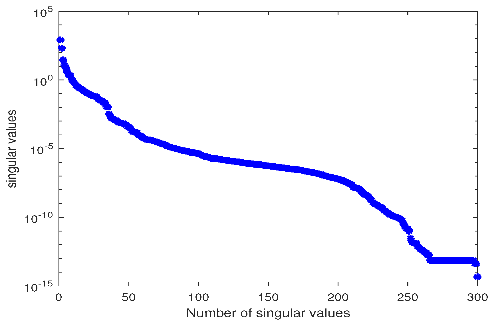
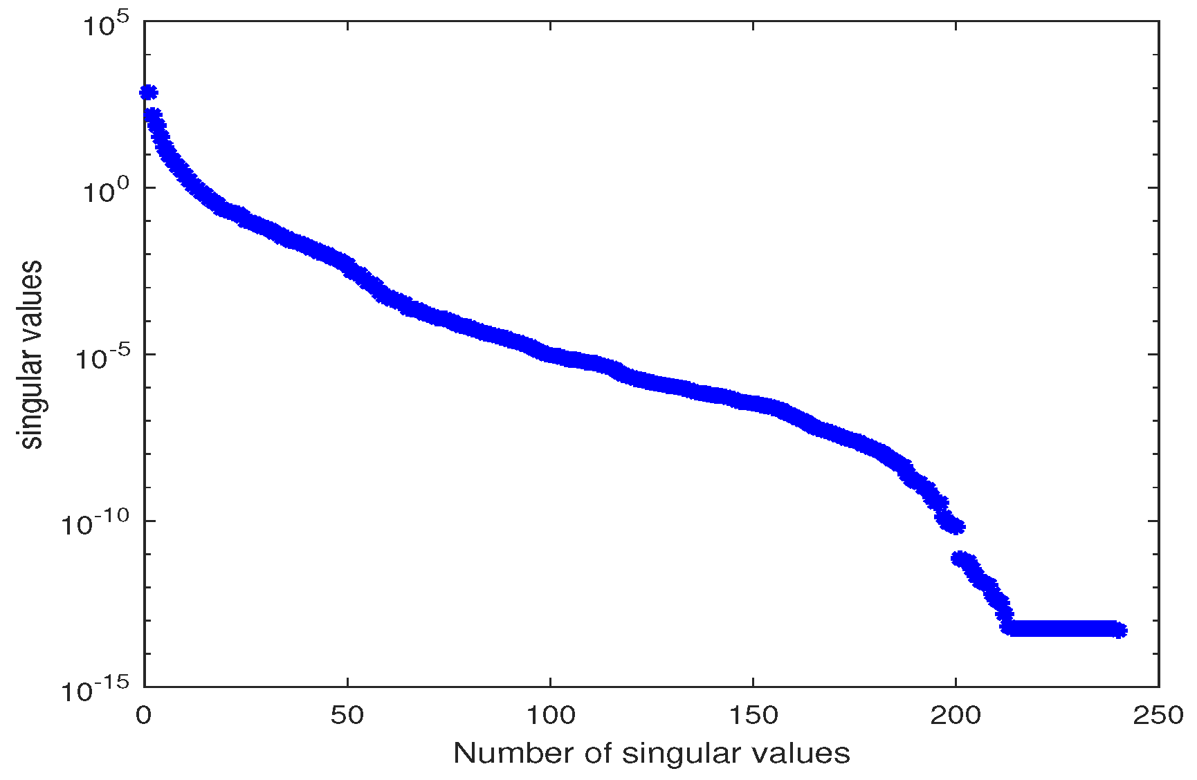
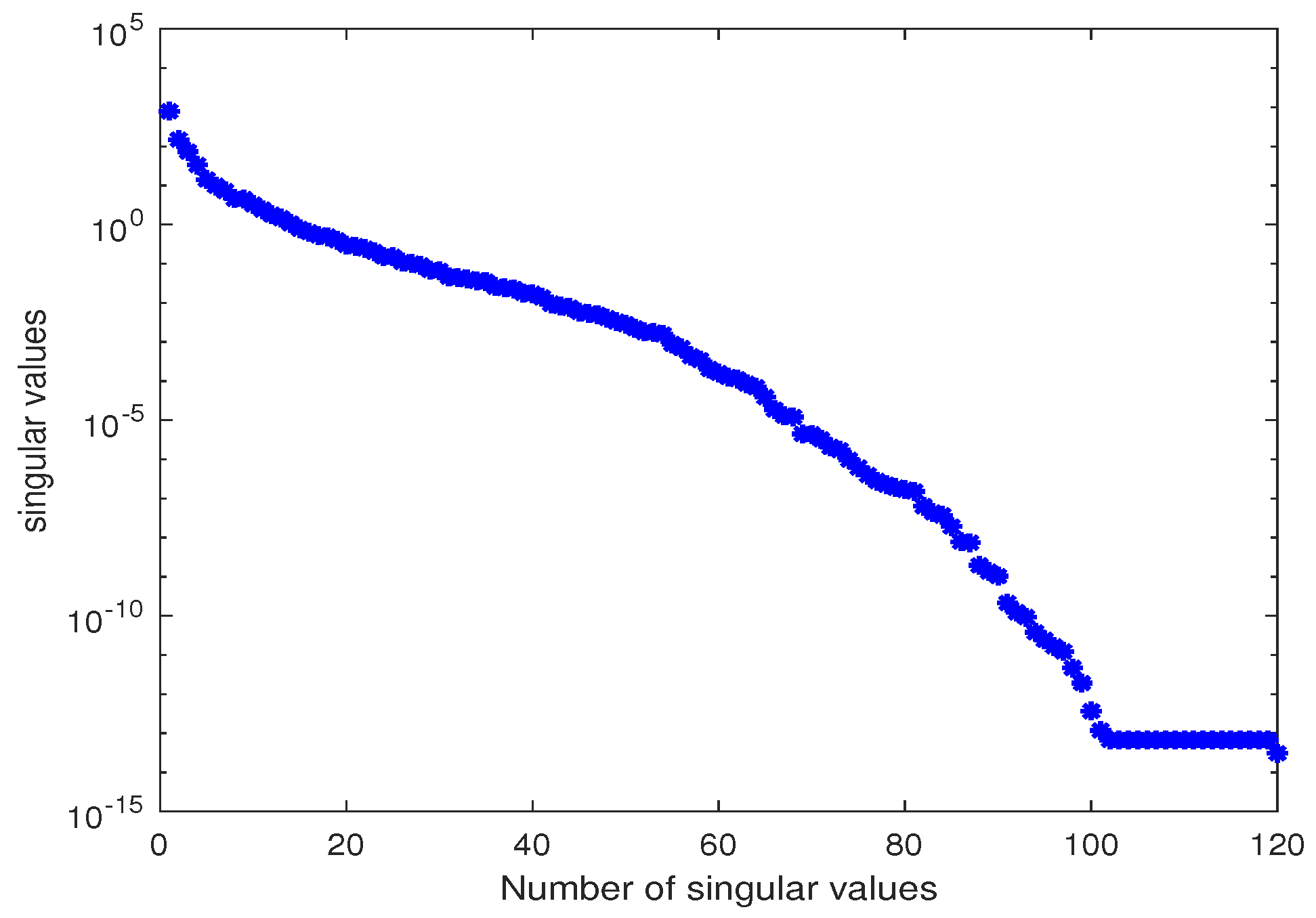
2.2. Computing the Reduced Basis

To obtain a reduced basis, one can use the eigenvalues of the correlation matrix C = X T X as in [24,25]. Since the eigenvalues λ j of C, and the singular values σ j of X are related as λ j = σ j 2 , we use a singular value decomposition (SVD) to compute the singular values of X instead.
If the matrix X has the condition number κ ( X ) , then the condition number of C is κ ( C ) = κ ( X ) 2 , such that for problems with high condition number the computation of eigenvalues is much less robust that the computation of singular values, see e.g., [31].
Let d = r a n k ( X ) m i n ( n m · n s , n t ) . The SVD guarantees the existence of real numbers σ 1 σ 2 σ d > 0 and orthogonal matrices V R n m · n s × n m · n s with columns { v i } i = 1 n m · n s and W R n t × n t with columns { w i } i = 1 n t , such that
V T X W = D 0 0 0 = : Σ R n m . n s × n t
where D = d i a g ( σ 1 , , σ d ) R d × d and the zeros denote matrices of appropriate dimensions. From (3), we obtain
X = V Σ W T ,
or similarly, the vectors { v i } i = 1 d and { w i } i = 1 d satisfy
X w i = σ i v i v i = 1 σ i X w i , for i = 1 , , d .
To obtain a reduced basis we can now cut off singular values with σ i < ε , where ε is chosen such that a smaller number of basis elements n r < < n m · n s is sufficient to capture the main features of the solution of (2). By setting V r = [ v 1 , , v n r ] R n m · n s × n r (the so-called POD modesor POD basis vectors), then a reduced order model (ROM) for (2) is given by
x ¯ ˙ r = f ¯ r ( t , x ¯ r ) , x ¯ r ( t 0 ) = V r T x ¯ 0 R n r ,
where x ¯ V r x ¯ r , i.e.,  V r x ¯ r serves as approximation for x ¯ , and  f ¯ r ( t , x ¯ r ) : = V r T f ¯ ( t , V r x ¯ r ) .
It is well-known that s p a n { v 1 , , v n r } is the best approximation of R a n g e ( X ) in the sense that minimizes the two-norm of the approximation error:
j = 1 n t x ¯ ( t j ) V r V r T x ¯ ( t j ) 2 2 = i = n r + 1 d σ i 2 ,
see  [32].
Usually, the goal is to choose n r small enough while the relative information content  [33] of the basis for the n r -dimensional subspace, defined by
I ( n r ) = i = 1 n r σ i i = 1 d σ i ,
is near to one. If the n r -dimensional subspace should contain a percentage p of the information contained in the full dimensional space R n m · n s , then one should choose n r such that
n r = argmin I ( n r ) | I ( n r ) p 100 .
Each data vector x ¯ i R n m · n s , i.e., the i-th column of X, can be written as
x ¯ i = j = 1 d b i j v j , with b i j = v j , x ¯ i = ( v j ) T · x ¯ i ,
where . , . denotes the canonical inner product in R n m · n s .
Thus, the state vector can be approximated in the reduced basis as
x ¯ i j = 1 n r b i j v j , i = 1 , , n t ,
and each n m -dimensional component x ¯ i , = 1 , , n s of x ¯ i (relating to (1)) can be represented in the reduced basis by
x ( t i ; Θ ) = x ¯ i j = 1 n r b i j v ^ j ,
where v j is decomposed into n s components as in (2)
v j = v 1 j v n m j v n m + 1 j v 2 n m j v ( n s 1 ) n m + 1 j v n m · n s j = : v ^ 1 j v ^ 2 j v ^ n s j .
Or analogously (in a continuous version of POD) as
x ( t ; Θ ) j = 1 n r b j ( t ) v ^ j ,
for coefficient functions b j ( t ) = x ( t ; Θ ) , v ^ j .

2.3. Construction of Data-Fitting Function

Next, we want to construct a data-fitting function Ψ ( t ) R n m that fits the known experimental data for the component k = 1 , , n d . We assume Ψ ( t ) to be of the form
Ψ ( t ) : = = 1 n s c x ¯ k ( t ) = = 1 n s c x ( t ; Θ ) .
With (6), we obtain
Ψ ( t ) = = 1 n s c j = 1 n r b j ( t ) v ^ j = = 1 n s j = 1 n r c x ( t ; Θ ) , v ^ j v ^ j .
Usually only a few specific states of the dynamical system can be measured in experiments. Here, we assume that the first n d components of the state vector can be measured and we want to determine the coefficients c in such a way that the first n d components of Ψ = [ Ψ k ] k = 1 n d are an acceptable fit of the experimental data points, i.e.,  Ψ k ( τ s ) y k ( τ s ) for s = 1 , , n τ and k = 1 , , n d .
Thus, we construct a linear system to be solved for c :
y k ( τ s ) = ! Ψ k ( τ s ) = = 1 n s j = 1 n r c b j ( τ s ) v ^ j k = = 1 n s j = 1 n r c x ( τ s ; Θ ) , v ^ j v ^ j k
for all k = 1 , , n d and s = 1 , , n τ .
We obtain n d · n τ equations for the n s unknowns c , = 1 , , n s . For each k = 1 , , n d , we obtain a linear system
A k c = y k
where A k = [ a s k ] , and  a s k : = j = 1 n r b j ( τ s ) V ( ( 1 ) n m + k , j ) , for = 1 , , n s , s = 1 , , n τ and y k = y k ( τ 1 ) y k ( τ n τ ) . Summarizing all A k and y k into one large system yields A c = y with A R n d n τ × n s and y R n d n τ .

2.4. Estimating the Parameters

Once we have a representation for Ψ ( t ) we can substitute Ψ and
Ψ ˙ i Ψ ( t i + 1 ) Ψ ( t i ) h s
as approximation for Ψ ˙ i into the ODE (1) at the simulation time points t i to obtain
Ψ ( t i + 1 ) Ψ ( t i ) h s f ( t i , Ψ ( t i ) , θ ) , i = 1 , , n t .
Here, Ψ can be assumed to be smooth since it is composed as linear combination of solution of an ODE. Inserting all information that we have gives
Ψ ( t i + 1 ) Ψ ( t i ) h s = f ( t i , Ψ ( t i ) , θ ) = 1 n s c x ( t i + 1 ; Θ ) = 1 n s c x ( t i ; Θ ) h s = f ( t i , = 1 n s c x ( t i ; Θ ) , θ ) .
This system can be solved for the parameter θ by a nonlinear system solver (e.g., fsolve in Matlab). We can sum up all these steps in the following Algorithm 1.
Algorithm 1 Parameter estimation for a kinetic model.
1.
Compute n s solutions of a kinetic model given by (1) for different parameter values Θ 1 , , Θ n s and form the snapshot matrix X.
2.
Compute the SVD of X. Truncate and remain only the most dominant singular values n r to obtain the POD basis.
3.
Express every vector in the snapshot matrix X as linear combination of the POD basis x ¯ i = j = 1 n r b i j v j with b i j = ( v j ) T · x ¯ i for i = 1 , , n t .
4.
Construct a data-fitting function that fits the known experimental data ( y ( τ s ) ) as a linear combination of POD basis Ψ ( t ) : = = 1 n s c x ¯ i ( t ) .
5.
Solve the linear system Ψ ( τ s ) = y ( τ s ) , s = 1 , , n τ to obtain the value of c l , l = 1 , , n s .
6.
Substitute the value of ψ into the original model Ψ ( t i + 1 ) Ψ ( t i ) h s f ( t i , Ψ ( t i ) , θ ) , i = 1 , , n t and solve the system for θ parameter.

3. Application of the Parameter Estimation Method to a Kinetic Model of CCR in E. coli

In this section, we apply the parameter estimation procedure introduced in the previous section to the kinetic model of carbon catabolite repression (CCR) in E. coli [28]. CCR is the main regulatory mechanism in E. coli for the control of carbohydrate uptake. The regulatory network is strongly hierarchical with a regulator Crp (cyclic AMP receptor protein) on the top. Crp serves as accelerator for gene expression in case of low C source availability and in this way coordinates different subsystems of the cell, responsible for the uptake of carbon sources, their breakdown for the production of energy and precursors, and the conversion of the latter to biomass. In the second level, substrate specific regulator proteins (main repressor proteins) are inactivated in case the specific substrate is available in the growth medium. The interplay between regulators and the transcription apparatus results for example in the observation that only one substrate is taken up although two substrates are provided in the beginning. Two distinct growth phases are observed, and a sequential uptake of the substrates take place (diauxic growth).

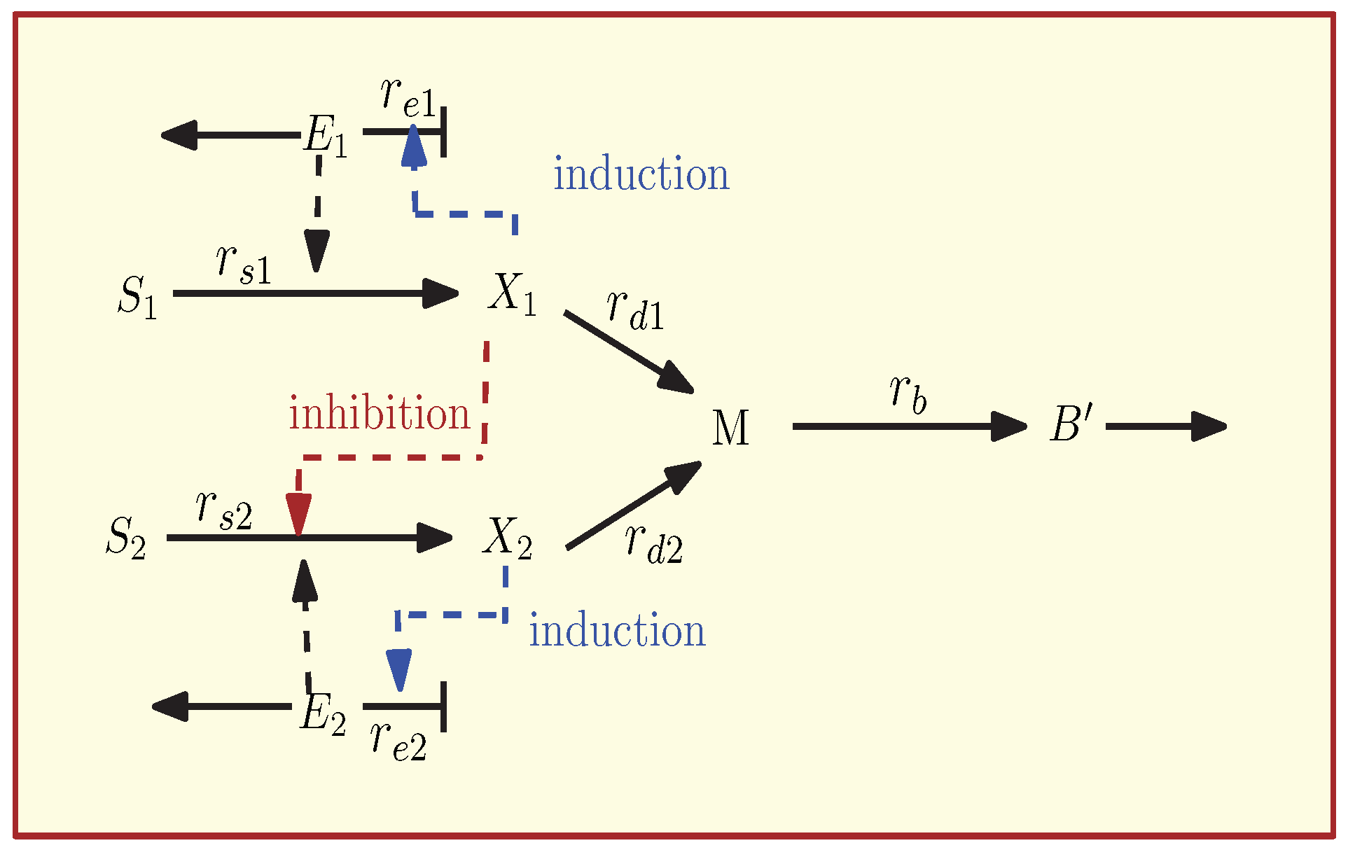
3.1. The Kinetic Model of the Carbon Catabolite Repression

The main structure of the reaction scheme is outlined in Figure 1. Two extracellular substrates ( S 1 and S 2 ) are taken up in enzyme catalysed reactions by their respective specific transporters ( E 1 and E 2 ). The substrates have representatives inside the cell ( X 1 and X 2 ). For example, in the case of glucose, X 1 represents the phosphorylated form glucose 6-phospahte while in the case of lactose, the substrate is not modified during the transport step. In general, transport systems for carbohydrate are inducible, that is, metabolites in the cell activate gene expression of the respective enzymes. In the model, these mechanisms are represented by a positive feedback from the X i to the synthesis of the respective enzymes E i (dashed blue lines). A special case for the interaction between two uptake systems in case of glucose and lactose is inducer exclusion (red dashed line); high levels of X 1 inhibit the activity of the second transporter for lactose uptake. The inhibition is so strong that the level of X 2 is minimal and, this way, the transporter E 2 cannot be synthesized. Only after they run out of glucose, the level of X 1 decreases and the inhibition is degraded. Both uptake branches converge in the central pathways, represented by metabolite M. From M, the synthesis of the main biomass compartment B is described with a single reaction.
The system of differential equations associated with the chemical reactions network is given by
x ˙ ( t ) = N · r ( x ( t ) ) ,
where x = [ S 1 , S 2 , X 1 , X 2 , E 1 , E 2 , M , B ] T R 8 is the vector of metabolite concentrations, r = [ r s 1 , r s 2 , r d 1 , r d 2 , r e 1 , r e 2 , r b ] T is the vector of reaction rates and N is the stoichiometric matrix given as follows:
N =   r s 1 r s 2 r d 1 r d 2 r e 1 r e 2 r b S 1 S 2 X 1 X 2 E 1 E 2 M B [ 1 0 0 0 0 0 0 0 1 0 0 0 0 0 0 0 1 0 0 0 0 0 0 0 1 0 0 0 0 0 0 0 1 0 0 0 0 0 0 0 1 0 0 0 1 1 0 0 1 0 0 0 0 0 0 1 ] R 8 × 7 .
The kinetic rate laws r s 1 , r s 2 are defined by Michaelis–Menten kinetics [34] and r d 1 , r d 2 , r e 1 , r e 2 , r b by mass action kinetics [35] as follows:
r s 1 = k s 1 E 1 S 1 K 1 + S 1 , r s 2 = k s 2 E 2 S 2 K 2 + S 2 , r e 1 = k e 1 f 1 , r e 2 = k e 2 f 2 , r d 1 = k x 1 X 1 , r d 2 = k x 2 X 2 , r b = k m M ,
where k x 1 , k x 2 , and  k m are the constant rates all in 1/h unit, K 1 , K 2 are the Michaelis–Menten constant in g/L unit and k e 1 , k e 2 are the constant rates in the mol/gDW.h. The turnover number of enzymes k s 1 , k s 2 is in the unit 1/h.
The system of ordinary differential equations of the carbon catabolite repression is given by
S i ˙ = r s i w i B , i = 1 , 2 X i ˙ = r s i r d i , E i ˙ = r e i μ E i , M ˙ = r d 1 + r d 2 r b , B ˙ = μ B , B ˙ = r b μ B ,
where w i is the molecular weight of the substrates (g/mol). The main biomass compartment B consists of macromolecular species like protein, DNA, RNA, lipid, etc., and variable B is the entire biomass, growing with the specific growth rate μ . The growth rate μ = Y 1 r s 1 + Y 2 r s 2 has the unit 1/h and Y 1 , Y 2 are yield coefficients with unit gDW/mol. The process of induction is described with rates f 1 , f 2 that are expressed in the following form
f 1 = X 1 β 1 + X 1 , f 2 = X 2 β 2 + X 2 ,
where β 1 , β 2 are in the unit mol/gDW and k 1 , k 2 are constant rates in mol/gDW.h unit. The intracellular components are assumed to be at the steady state i.e., X 1 ˙ = 0 , X 2 ˙ = 0 , and  M ˙ = 0 . This case study considers inducer exclusion where metabolite X 1 works as a regulatory metabolite and inhibits enzyme E 2 which is responsible for substrate S 2 uptake. In a scheme, this is represented by an extension of the uptake rate r s 2 to r s 2 · α α + X 1 , where α is a constant. Then the kinetic model of the above network is given as follows
S 1 ˙ = k s 1 · E 1 · S 1 K 1 + S 1 · w 1 · B , S 2 ˙ = k s 2 · E 2 · S 2 K 2 + S 2 · w 2 · B · f i n h i b i t , E 1 ˙ = k e 1 X 1 β 1 + X 1 μ E 1 , E 2 ˙ = k e 2 X 2 β 2 + X 2 μ E 2 , B ˙ = μ B , B ˙ = k m · M μ B ,
where
X 1 = k s 1 · E 1 · S 1 k x 1 ( K 1 + S 1 ) , X 2 = k s 2 · E 2 · S 2 k x 2 ( K 2 + S 2 ) · f i n h i b i t M = k x 1 · X 1 k m + k x 2 · X 2 k m , f i n h i b i t = α α + X 1 .

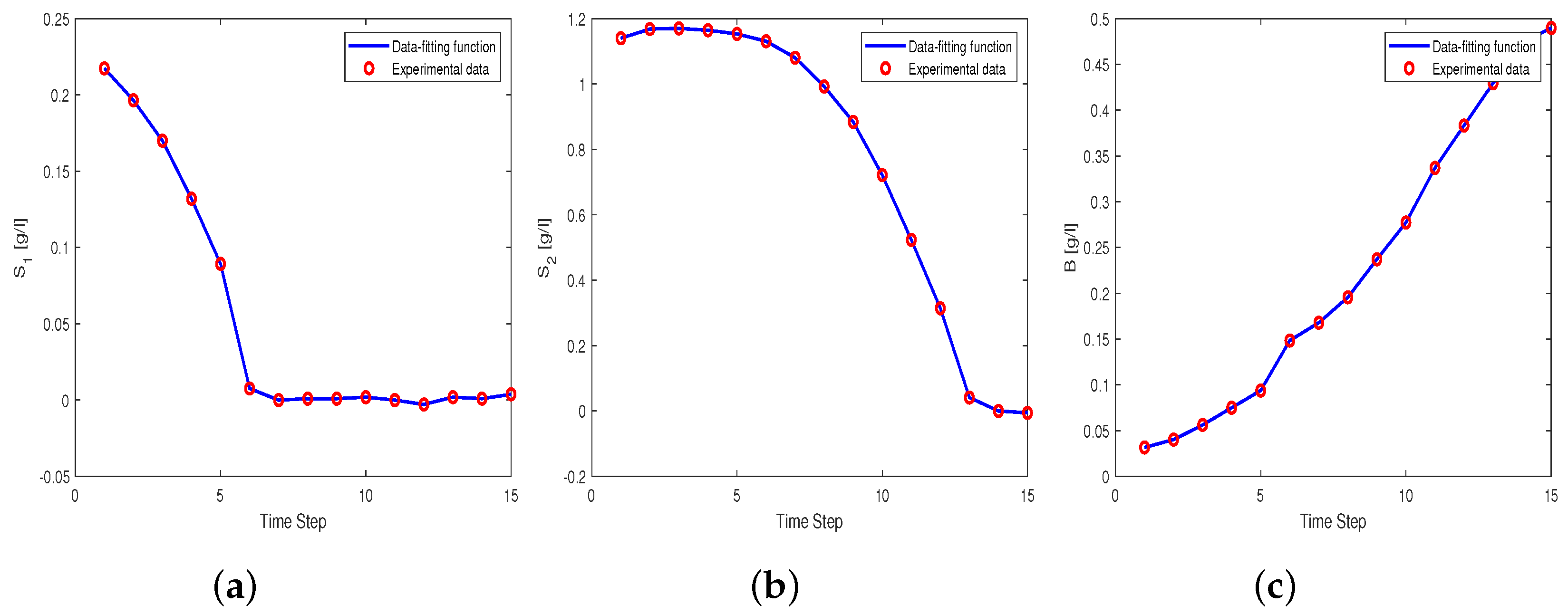
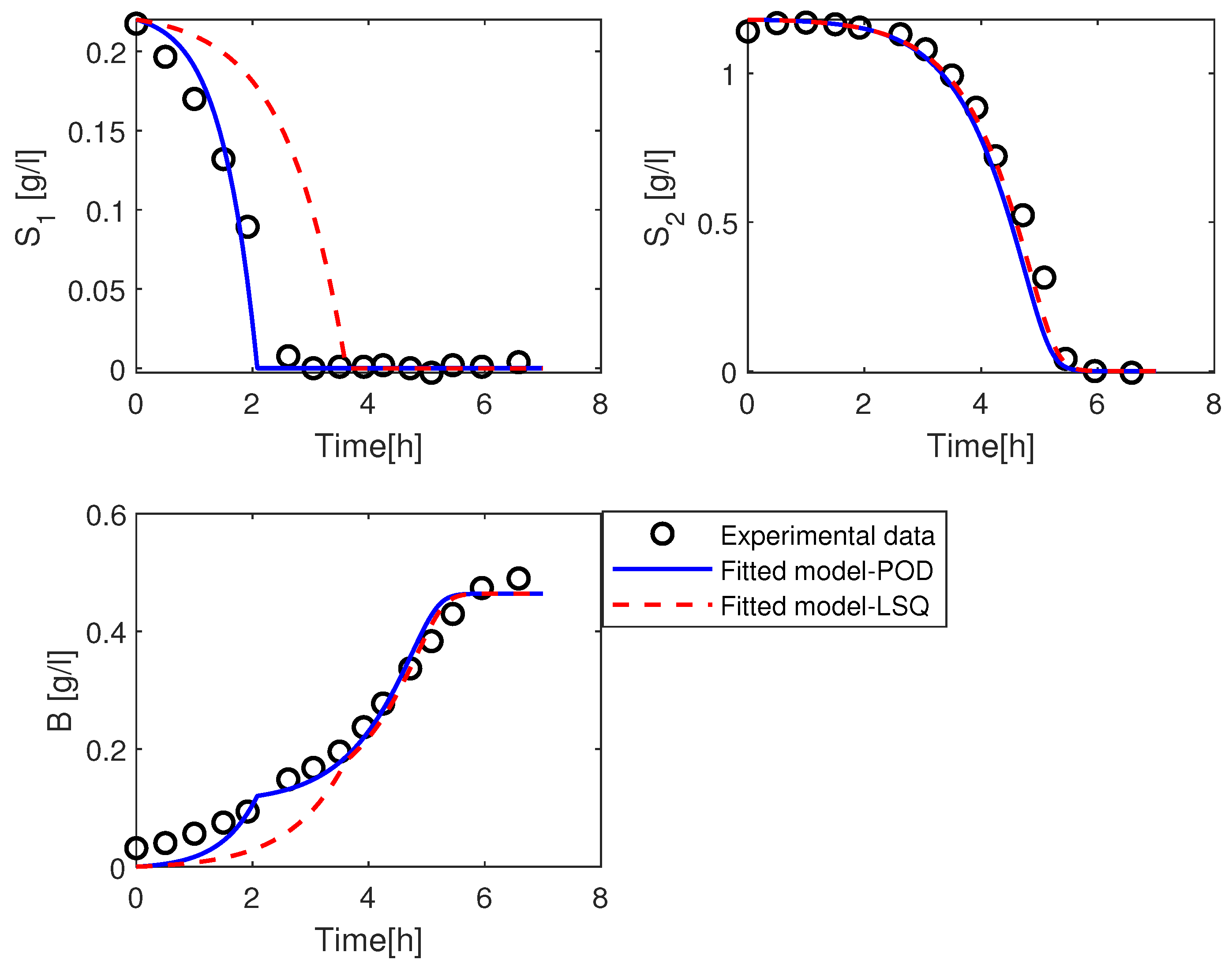
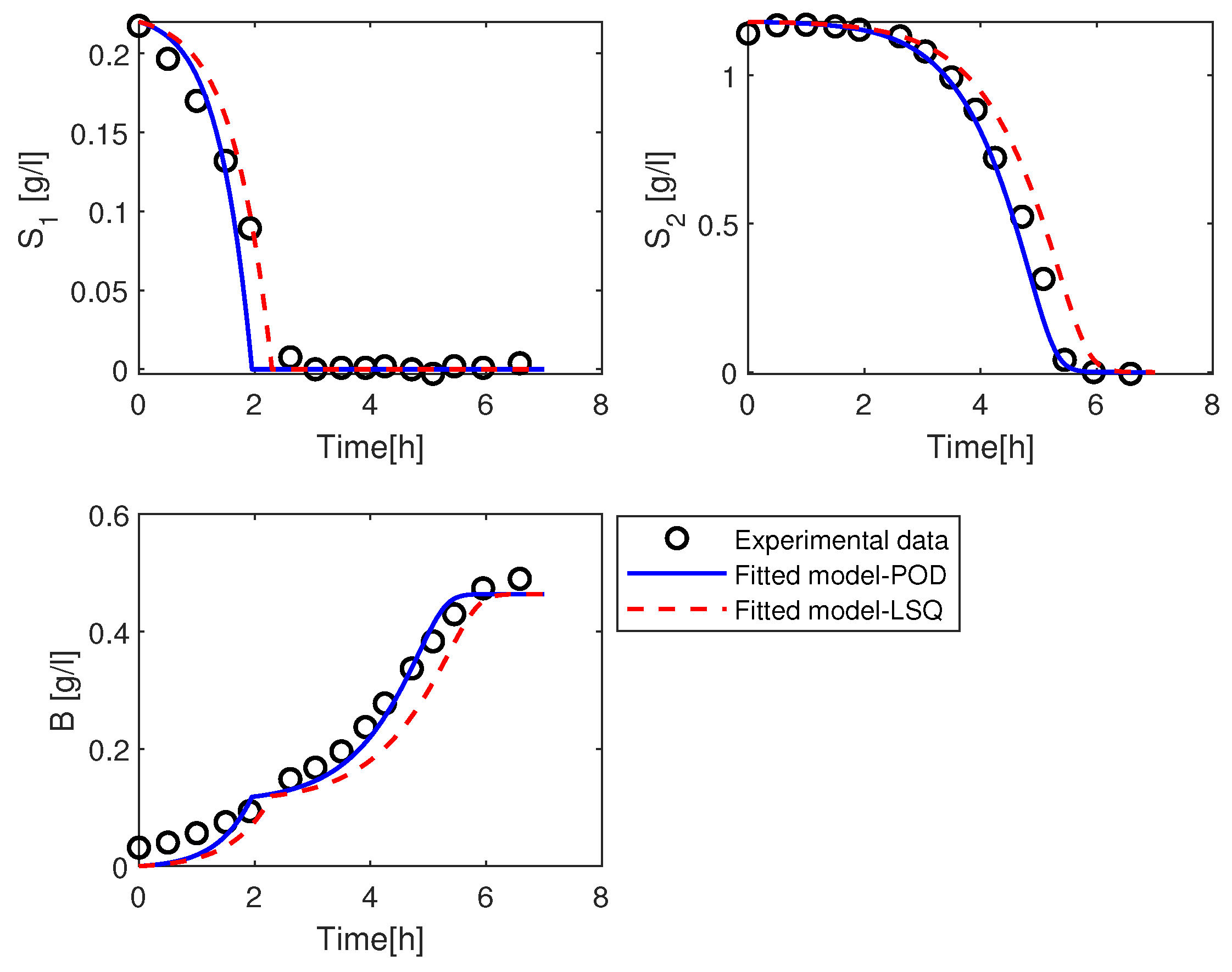
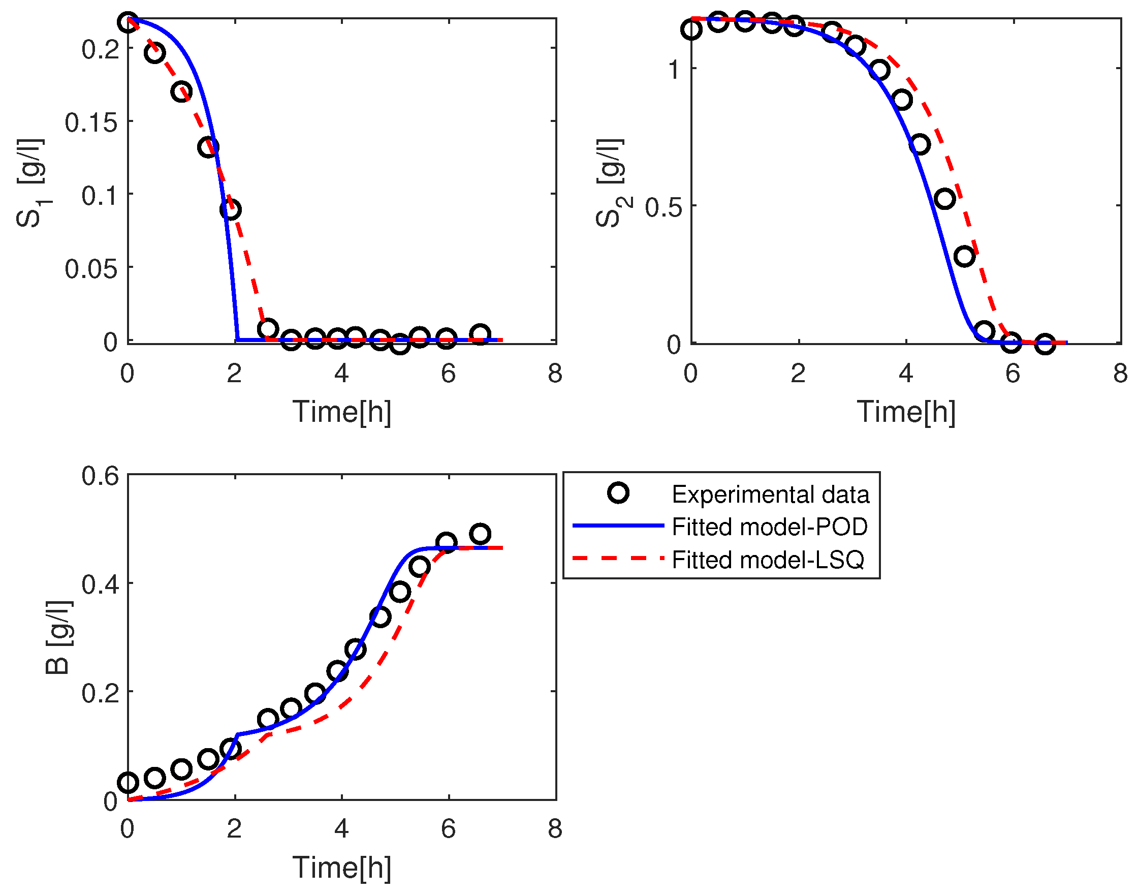
3.2. Numerical Results

In the following we present some examples in which we estimate certain parameter values of the kinetic model (7). All results presented in the following sections were computed with MATLAB (R2022a).

3.2.1. Estimation of the Parameter k s 1

In this first example we estimate one parameter value, namely, the uptake rate constant k s 1 . First, we compute the snapshot matrix X from the simulation of the kinetic model (7) for different values of the parameter k s 1 over the time interval [ 0 , 7 ] h. The different values of parameter k s 1 are equidistantly distributed in the interval [ 10 5 , 10 2 ] , which are the lower and upper bound of parameter value, respectively. In each of n s simulation, we evaluate at n t simulation time points. In this example, we set n s = 50 . The remaining constant reaction rates are given in Table 1 and the parameter value of k s 2 = 0.0033 is assumed. We use the MATLAB function ode15s with tolerances R T O L = A T O L = 10 6 to compute a numerical solution of the ODE system (7) with 50 different values for the parameter k s 1 . The initial concentrations of extracellular and intracellular metabolites are assumed to be ( S 1 , S 2 , E 1 , E 2 , B , B ) = ( 0.22 , 1.18 , 0.1 , 0.1 , 0.032 , 0.5 ) R 6 .
We used the MATLAB function svd to calculate the singular value decomposition of X. The singular values are shown in Figure 2.
The behavior of the model order reduction method strongly depends on the decay of the singular values of the snapshot matrix. Figure 2 shows gradually decaying singular values with a strong decay for the smallest singular values indicating that ignoring these will not lead to any considerable loss of information. We truncate the most dominant singular values such that the relative information coefficient I is close to one. In this example, we use n r = 60 where I = 0.99 . The date-fitting function Ψ ( t ) is constructed as in Section 2.3 to fit the experimental data set for the three measurement components S 1 , S 2 , and B at the measurement time points n τ = 15 . The trajectories of the measurement data set and the data-fitting function are depicted in Figure 3.
We can observe that the data-fitting function fits well with the measurement data. Once the data-fitting function Ψ ( t ) is obtained, we can substitute the function Ψ ( t ) in the kinetic model (7) and solve the system for the parameter k s 1 . We use the MATLAB function fsolve with function tolerance T O L = 10 6 using the Levenberg–Marquardt algorithm with initial guess k s 1 = 0.0167 . The solution gives an estimated parameter value of k b e s t = 0.018 . For the purpose of comparison, we also provide results from the least square method (LSQ). We perform the LSQ method using MATLAB function lsqnonlin and lhsdesign with the same assumptions (e.g., number of fits n s and lower and upper bounds) as in the POD method. The solution gives an estimated value k l s q = 0.01 of the parameter k s 1 . The simulation results of the kinetic model with k b e s t in comparison with the simulation results of the kinetic model with k l s q , and the measurement data are depicted in Figure 4.
We can observe that the dynamical behavior of the kinetic model states with parameter value k b e s t matches well with the experimental data for the substrates S 1 , S 2 , and the Biomass B. While the simulation of the solution of the kinetic model with parameter value k l s q for the substrate S 1 is unable to match well with the data. The substrate S 1 spends more time to consume compared to the measured data. In contrast, the trajectories of S 2 and Biomass still fit good with the measured data. From the above figure, the POD method gives better results than the LSQ method. Note, that with a change of the lower and upper bounds in the LSQ method, we could obtain a better result. Both methods are sensitive to assumptions, which means that the lower and upper bound of parameter value l b , u b , the mesh size M, and the reduced basis n r can be adjusted to obtain a good fitting.

3.2.2. Estimation of the Parameters k s 1 and k s 2

In this example, we consider the two parameters for the uptake rate constants k s 1 and k s 2 . The snapshot matrices X is computed from n s = 40 simulation of the kinetic model equations (7) over the time interval. We use a Latin hypercube sampling (LHS) to obtain different values of the parameters via the MATLAB function lhsdesign. To generate parameter sampling for the parameters k s 1 and k s 2 , we set the lower and upper bound for the parameters as l b = 10 5 , u b = 10 2 . We use the MATLAB function svd to calculate the singular value decomposition of X. The singular values are depicted in Figure 5.
Here, we truncate at n r = 60 , with relative information coefficient I = 0.9 . Substituting ψ in the kinetic model and solving the system for the two parameters using MATLAB function fsolve with function tolerance 10 6 and initial guesses k s 1 = 0.0167 , k s 2 = 0.0033 , we obtain the estimated values of the parameters k b e s t = [ 0.0194 , 0.0032 ] . In this example, we perform the LSQ method with different assumptions of bounds. We set the lower and upper bounds in the LSQ method to be l b = 10 3 , u b = 10 1 , we obtain the estimated values k l s q = [ 0.0163 , 0.0029 ] .
From Figure 6, we can observe that the trajectories for the experimental data and the simulation results of kinetic model with the estimated parameter values using POD method match good for the substrates trajectories S 1 , S 2 and Biomass curve. While the simulation of the kinetic model with parameters value using the LSQ method is slightly different from the measured data.

3.2.3. Estimation of the Parameters k s 1 , k e 1 , k x 1 and k x 2

In this example, we apply the method to estimate four parameters in the kinetic model (7). We use the MATLAB function lhsdesign to generate parameter sampling for the parameters k s 1 , k s 2 , k e 2 , and  β 2 , where the lower and upper bound for the parameters are [ 10 2 , 10 + 1 ] . We set the number of simulation to n s = 20 . The snapshot matrix X is computed and the SVD is applied; Figure 7 shows the singular values. We choose n r = 60 and the system is solved for the four parameters using MATLAB function lsqnonlin with options algorithm levenberg-marquardt and initial guess of parameters k s 1 = 0.0167 , k e 1 = 6 , k x 1 = 10 , and  k x 2 = 10 . The estimated values of the parameters are k b e s t = [ 0.01 , 125.7 , 103.6 , 9.97 ] . We perform the LSQ method using the same assumptions as in the POD method, the solution gives an estimated values k l s q = [ 0.059 , 0.084 , 0.333 , 9.99 ] .
At the beginning of the simulation, we can observe from Figure 8 that the trajectory of S 1 using the estimated values from the POD method consumes slowly compared to the trajectories by the LSQ method and the experimental data. Around the time 2 h, it is exhausted a bit earlier than other curves. The trajectories of S 2 and B from the POD method are qualitatively similar to the measured data while their trajectories of the LSQ method are slightly different.

4. Conclusions and Discussion

In this paper, we have discussed the parameter estimation procedure using model order reduction by the POD method for a kinetic model of a cellular system. The process of finding parameter values is considered to be a main challenge in mathematical modelling of biological system, so the possibility to use the POD method in the parameter estimation problem is of crucial importance. We have applied the POD method and the singular value decomposition to obtain the reduced basis elements, which are used for constructing a function that fits the trajectory of the kinetic model to the observable data set of the biological system. The parameter estimation using the POD method is capable to estimate the uptake rate constants and other parameters of the CCR kinetic model. The solution of the kinetic model with the estimated parameter values matches good with the experimental data set. We performed the least square method to estimate parameter values of the CRR kinetic model for the sake of comparison with the POD method and show to what extent the POD method could estimate the values of parameters of the CRR kinetic model. We could observe that the number of reduced basis, the lower and upper bounds, and the number of simulations play an important role in the parameter estimation problem. For every parameter estimation case, these numbers can be adjusted until the desired results are obtained. In addition, the presented algorithm of parameter estimation can be used as a reference for different kinetic models of biological systems. The presented approach has some limitations as it strongly depends on the behavior of the singular value spectrum. If there is only a small number of dominant eigenmodes, then the singular values will rapidly decay and only a small number of them is enough to capture the characteristic behavior of the system. However, in some ill-posed cases, this might not be the case and the heuristic approach presented in the algorithm might not lead to satisfactory results. The choice of a suitable threshold for discarding certain singular values also depends on the quality of the data, in particular, rounding and approximation errors. It has been shown in [36] that the truncated SVD is a suitable method for the regularization of an ill-posed problem when the coefficient matrix is ill-conditioned with a well-determined numerical rank. In this case, the solution obtained by the truncated SVD with a truncation threshold equal to the numerical rank of the matrix is guaranteed to be similar to the regularized solution where the regularization parameter is chosen near its intuitive optimum value.

Author Contributions

N.A.E. and L.S. designed the study. N.A.E. performed the simulation studies and wrote the first draft of the paper. A.K. provided a kinetic model for the CCR network. All authors discussed the results. All authors have read and agreed to the published version of the manuscript.

Funding

N.A.E. was supported by Postdoc Scholarship from the Egyptian Ministry of Higher Education (Cultural Affairs and Missions Sector). L.S. was supported by the Berlin Mathematics Research Center MATH+.

Data Availability Statement

Not applicable.

Acknowledgments

We acknowledge support by the German Research Foundation and the Open Access Publication Fund of TU Berlin.

Conflicts of Interest

The authors declare no conflict of interest.

References

  1. Mannan, A.A.; Toya, Y.; Shimizu, K.; McFadden, J.; Kierzek, A.M.; Rocco, A. Integrating kinetic model of E. coli with genome scale metabolic fluxes overcomes its open system problem and reveals bistability in central metabolism. PLoS ONE 2015, 10, e0139507. [Google Scholar] [CrossRef] [PubMed] [Green Version]
  2. Lima, A.P.; Baixinho, V.; Machado, D.; Rocha, I. A comparative analysis of dynamic models of the central carbon metabolism of Escherichia coli. IFAC-PapersOnLine 2016, 49, 270–276. [Google Scholar] [CrossRef] [Green Version]
  3. Ali Eshtewy, N. Mathematical Modeling of Metabolic-Genetic Networks; Freie Universität Berlin: Berlin, Germany, 2020. [Google Scholar]
  4. Aster, R.C.; Borchers, B.; Thurber, C.H. Parameter Estimation and Inverse Problems; Elsevier: Amsterdam, The Netherlands, 2018. [Google Scholar]
  5. Moles, C.G.; Mendes, P.; Banga, J.R. Parameter estimation in biochemical pathways: A comparison of global optimization methods. Genome Res. 2013, 13, 2467–2474. [Google Scholar] [CrossRef] [PubMed] [Green Version]
  6. Tarantola, A. Inverse Problem Theory and Methods for Model Parameter Estimation; SIAM: Philadelphia, PA, USA, 2005; Volume 89. [Google Scholar]
  7. Zhdanov, M.S. Inverse Theory and Applications in Geophysics; Elsevier: Amsterdam, The Netherlands, 2015; Volume 36. [Google Scholar]
  8. Parker, R.L. Understanding inverse theory. Annu. Rev. Earth Planet. Sci. 1977, 5, 35–64. [Google Scholar] [CrossRef]
  9. Kreutz, C. An easy and efficient approach for testing identifiability. Bioinformatics 2018, 34, 1913–1921. [Google Scholar] [CrossRef] [Green Version]
  10. Raue, A.; Schilling, M.; Bachmann, J.; Matteson, A.; Schelke, M.; Kaschek, D.; Hug, S.; Kreutz, C.; Harms, B.D.; Theis, F.J.; et al. Lessons Learned from Quantitative Dynamical Modeling in Systems Biology. PLoS ONE 2013, 8, e74335. [Google Scholar] [CrossRef]
  11. Deuflhard, P. Newton Methods for Nonlinear Problems: Affine Invariance and Adaptive Algorithms; Springer: Berlin/Heidelberg, Germany, 2011; Volume 35. [Google Scholar]
  12. Altman, N.; Krzywinski, M. Points of Significance: Simple Linear Regression; Nature Publishing Group: London, UK, 2015. [Google Scholar]
  13. Björck, Å. Numerical Methods for Least Squares Problems; Society for Industrial and Applied Mathematics: Philadelphia, PA, USA, 1996. [Google Scholar]
  14. Enders, C.K. Maximum likelihood estimation. In Encyclopedia of Statistics in Behavioral Science; Wiley: Hoboken, NJ, USA, 2005. [Google Scholar]
  15. Rudi, J.; Bessac, J.; Lenzi, A. Parameter Estimation with Dense and Convolutional Neural Networks Applied to the FitzHugh—Nagumo ODE. Math. Sci. Mach. Learn. 2022, 781–808. [Google Scholar] [CrossRef]
  16. Kerschen, G.; Golinval, J.; Vakakis, A.F.; Bergman, L.A. The method of proper orthogonal decomposition for dynamical characterization and order reduction of mechanical systems: An overview. Nonlinear Dyn. 2005, 41, 147–169. [Google Scholar] [CrossRef]
  17. Volkwein, S. Proper orthogonal decomposition: Theory and reduced-order modelling. Lect. Notes Univ. Konstanz 2013, 4, 1–29. [Google Scholar]
  18. Karhunen, K. Über lineare Methoden in der Wahrscheinlichkeitsrechnung. Ann. Acad. Sci. Fenn. Ser. A Math. Phys. 1947, 47, 1–79. [Google Scholar]
  19. Loeve, M. Elementary Probability Theory; Springer: Berlin/Heidelberg, Germany, 1977; pp. 1–52. [Google Scholar]
  20. Benner, P.; Goyal, P.; Heiland, J.; Duff, I.P. Operator inference and physics-informed learning of low-dimensional models for incompressible flows. arXiv 2020, arXiv:2010.06701. [Google Scholar] [CrossRef]
  21. Cazemier, W.; Verstappen, R.W.C.P.; Veldman, A.E.P. Proper orthogonal decomposition and low-dimensional models for driven cavity flows. Phys. Fluids 1998, 10, 1685–1699. [Google Scholar] [CrossRef]
  22. Luo, Z.; Chen, J.; Navon, I.M.; Yang, X. Mixed finite element formulation and error estimates based on proper orthogonal decomposition for the nonstationary Navier–Stokes equations. SIAM J. Numer. Anal. 2009, 47, 1–19. [Google Scholar] [CrossRef] [Green Version]
  23. Ali Eshtewy, N.; Scholz, L. Model Reduction for Kinetic Models of Biological Systems. Symmetry 2020, 12, 863. [Google Scholar] [CrossRef]
  24. Rehm, A.M.; Scribner, E.Y.; Fathallah-Shaykh, H. Proper orthogonal decomposition for parameter estimation in oscillating biological networks. J. Comput. Appl. Math. 2014, 258, 135–150. [Google Scholar] [CrossRef]
  25. Ly, H.V.; Tran, H.T. Proper orthogonal decomposition for flow calculations and optimal control in a horizontal CVD reactor. Q. Appl. Math. 2002, 60, 631–656. [Google Scholar] [CrossRef] [Green Version]
  26. Boulakia, M.; Schenone, E.; Gerbeau, J.-F. Reduced-order modeling for cardiac electrophysiology. Application to parameter identification. Int. J. Numer. Methods Biomed. Eng. 2012, 28, 727–744. [Google Scholar] [CrossRef] [Green Version]
  27. Kahlbacher, M.; Volkwein, S. Estimation of regularization parameters in elliptic optimal control problems by POD model reduction. In Proceedings of the IFIP Conference on System Modeling and Optimization, Cracow, Poland, 23–27 July 2007; Springer: Berlin/Heidelberg, Germany, 2007; pp. 307–318. [Google Scholar]
  28. Kremling, A.; Geiselmann, J.; Ropers, D.; De Jong, H. An ensemble of mathematical models showing diauxic growth behaviour. BMC Syst. Biol. 2018, 12, 82. [Google Scholar] [CrossRef]
  29. Helton, J.C.; Davis, F.J. Latin hypercube sampling and the propagation of uncertainty in analyses of complex systems. Reliab. Eng. Syst. Saf. 2003, 81, 23–69. [Google Scholar] [CrossRef] [Green Version]
  30. McKay, M.D.; Beckman, R.J.; Conover, W.J. A comparison of three methods for selecting values of input variables in the analysis of output from a computer code. Technometrics 2000, 42, 55–61. [Google Scholar] [CrossRef]
  31. Golub, G.H.; Van Loan, C.F. Matrix Computations, 3rd ed.; Johns Hopkins University Press: Baltimore, MD, USA, 1996. [Google Scholar]
  32. Hinze, M.; Volkwein, S. Model Order Reduction by Proper Orthogonal Decomposition. Konstanz. Schriften Math. 2019, 47–96. [Google Scholar] [CrossRef]
  33. Afanasiev, K.; Hinze, M. Adaptive Control of a Wake Flow Using Proper Orthogonal Decomposition. Lect. Notes Pure Appl. Math 2001, 216, 317–332. [Google Scholar]
  34. Michaelis, L.; Menten, M.L. Die Kinetik der Invertinwirkung. Biochem. Z. 1913, 49, 333–369. [Google Scholar]
  35. Guldberg, C.M.; Waage, P. Etudes Sur Les Affinités Chimiques; Brøgger & Christie: Christiania, Denmark, 1867. [Google Scholar]
  36. Per Christian, H. The truncatedSVD as a method for regularization. Bit Numer. Math. 1987, 27, 534–553. [Google Scholar]
Figure 1. Reaction scheme for the diauxic growth network. S 1 , S 2 are the substrates, X 1 , X 2 are the intracellular metabolites, E 1 , E 2 are the enzymes, M is the intermediate metabolite, and B is the main Biomass. The reaction rates are indicated in (solid arrows), catalytic activities and regulatory interactions in (dashed arrows).
Mathematics 11 00699 g001
Figure 2. Singular values of snapshot matrix X for estimating parameter k s 1 .
Mathematics 11 00699 g002
Figure 3. (a) trajectory of substrate S 1 using data-fitting function with a solid line and experimental data with a circle. (b) The trajectory of substrate S 2 . (c) The trajectory of Biomass B.
Mathematics 11 00699 g003
Figure 4. Simulation of the solution of the kinetic model with the parameter value k s 1 using POD method in blue (solid line), LSQ method in red (dashed line), and the experimental data in black (open circles).
Mathematics 11 00699 g004
Figure 5. Singular values of the snapshot matrix X for estimating Parameters k s 1 and k s 2 .
Mathematics 11 00699 g005
Figure 6. Simulation of the solution of the kinetic model with the parameters value k s 1 and k s 2 using POD method in blue (solid line), LSQ method in red (dashed line), and the experimental data in black (open circles).
Mathematics 11 00699 g006
Figure 7. Singular values of the snapshot matrix X for estimating parameters k s 1 , k e 1 , k x 1 and k x 2 .
Mathematics 11 00699 g007
Figure 8. Simulation of the solution of the kinetic model with the parameters value k s 1 , k e 1 , k x 1 and k x 2 using POD method in blue (solid line), LSQ method in red (dashed line), and the experimental data in black (open circles).
Mathematics 11 00699 g008
Table 1. The set of all parameters of the kinetic model that are taken from literature [28].
Constant RatesValueUnit
K 1 1 × 10 4 g/L
K 2 0.2 g/L
k e 1 6mol/gDWh
k e 2 8.69 mol/gDWh
k x 1 101/h
k x 2 101/h
k m 101/h
β 1 1mol/gDW
β 2 0.6 mol/gDW
α 11.05 mol/gDW
Y 1 90gDW/mol
Y 2 102.6 gDW/mol
w 1 180gDW/mol
w 2 342gDW/mol
Disclaimer/Publisher’s Note: The statements, opinions and data contained in all publications are solely those of the individual author(s) and contributor(s) and not of MDPI and/or the editor(s). MDPI and/or the editor(s) disclaim responsibility for any injury to people or property resulting from any ideas, methods, instructions or products referred to in the content.

