1. Introduction
In December 2019, an epidemic first appeared in Wuhan, China’s Hubei province. The cause of this epidemic was not clear, and the epidemic quickly spread to other countries. Not long after, this infectious disease of unknown cause was identified as a new coronavirus (nCoV) and this virus was named severe acute respiratory syndrome coronavirus 2 (SARS-CoV-2). The World Health Organization (WHO) named this infectious disease as coronavirus disease 2019 (COVID-19) and the SARS-CoV-2 epidemic was declared a pandemic on 11 March 2020. According to worldometer data, as of 25 December 2022, worldwide, there have been a total of 661,711,220 cases, 6,685,775 deaths, and 634,178,985 recoveries.
To address COVID-19, measures such as the mutual stoppage of countries’ flights, border closings, taking quarantine decisions for infected people, curfews, education suspension, and the beginning of distance education were taken. In addition, all kinds of cultural, scientific, artistic, and similar meetings and events were postponed. Places such as theatres, cinemas, massage parlors, gyms, cafes, concert halls and wedding halls were temporarily closed. Simultaneously, scientists started the vaccine studies and soon after, people tried to immunize the population by vaccinating them. Thus, the normalization process was begun. However, the number of cases and deaths is still increasing significantly. For this reason, all studies related to the pandemic are of great importance for science and humanity.
On the other hand, studies were also started in the field of mathematics for this pandemic with the help of the models related to infectious diseases. The most important of these model problems are the continuous population models [
1,
2,
3,
4,
5,
6,
7], the Lotka–Volterra population model [
2,
5,
6,
7,
8,
9,
10,
11,
12,
13,
14], the Hantavirus infection model [
15,
16,
17,
18,
19], the HIV infection models [
20,
21,
22,
23,
24,
25,
26,
27,
28,
29,
30,
31,
32,
33,
34,
35], the SIR epidemic model [
36,
37,
38,
39,
40,
41], and the SIRD epidemic model [
42,
43,
44,
45].
Canto, Avila–Vales and Garcia–Almeida studied a SIRD-based COVID-19 models in Yucatan, Mexico in 2020 [
46]. Canto and Avila–Vales worked on a parametric estimation of an SEIR and an SIRD models of COVID-19 pandemic in Mexico in 2020 [
47]. Calafiore, Novara, and Possieri investigated a modified SIR model for the COVID-19 contagion in Italy in 2020 [
48]. Calafiore and Novara studied a time-varying SIRD model for the COVID-19 contagion in Italy in 2020 [
49]. Mohammadi, Rezapour, and Jajarmi worked the fractional SIRD mathematical model for the first and second waves of the disease in Iran and Japan in 2021 [
50]. Pacheco and Lacerda made function estimation and regularization in an SIRD model applied to the COVID-19 pandemics in 2021 [
51]. Faruk and Kar conducted a data-driven analysis and prediction of COVID-19 dynamics during the third wave by using an SIRD model in Bangladesh in 2021 [
52]. Covid-19 epidemic data in Italy, using an adjusted time-dependent SIRD model, was modeled by Ferrari et al. in 2021 [
53]. Kovalnogov, Simos, and Tsitouras studied Runge–Kutta pairs suited for SIR-type epidemic models in 2021 [
54]. Martinez investigated a modified SIRD model to study the evolution of the COVID-19 pandemic in Spain in 2021 [
55]. Pei and Zhang made long-term predictions of COVID-19 in some countries by a SIRD Model in 2021 [
56]. The progress of the COVID-19 outbreak in India was worked by Chatterjee et al. in 2021 [
57] by using a SIRD model. Fern
ndez–Villaverde and Jones estimated and simulated an SIRD model of COVID-19 for many countries, states, and cities in 2022 [
58]. In addition, there are some studies in the literature regarding these models [
59,
60,
61,
62,
63].
In 2020, a novel parametric model of the COVID-19 to estimate the casualties in Turkey was studied by Tutsoy et al. [
64]. In 2020, the progress of COVID-19 in Turkey was estimated by Özdinç et al. [
65]. Three mathematical models for forecasting the COVID-19 outbreak in Iran and Turkey were assessed by Niazkar et al. in 2020 [
66]. The forecasting epidemic size for Turkey and Iraq using the logistic model was made by Ahmed et al. in 2020 [
67]. Atangana and Araz studied the mathematical model of COVID-19 spread in Turkey and South Africa in 2020 [
68]. Djilali and Ghanbari estimated analysis of the peak outbreak epidemic in South Africa, Turkey, and Brazil in 2020 [
69]. The dynamics of the outbreak in Hubei and Turkey were predicted and analyzed by Aslan et al. in 2020 [
70]. Atangana and Araz modeled third waves of COVID-19 spread with piecewise differential and integral operators for Turkey, Spain, and Czechia in 2021 [
71].
On the other hand, various numerical methods based on the Pell–Lucas polynomials were studied to obtain the approximate solutions of some differential equations and integro-differential equations [
7,
72,
73,
74,
75,
76,
77]. Accordingly, it is concluded that effective results are obtained with the help of the Pell–Lucas polynomials. To date, there is still no the collocation method based on the Pell–Lucas polynomials among the studies on the approximate solutions of the SIR model problem. Therefore, in this study, the parameters of the SIR model problem are determined according to Covid-19 data in Turkey and the Pell–Lucas collocation method is applied to this model.
In this study, the SIR epidemic model is considered in [
47,
52,
57]
with the initial conditions
where
. That is, population size
P is constant.
The descriptions of the parameters and the variables in the model (
1) and (
2) are given in
Table 1. Additionally, the arrows in
Figure 1 indicate the flow between the populations of susceptible
, infected
, removed
. Note that the individuals
in the model represents the number of individuals who both recovered and died.
Our aim is to find the Pell–Lucas polynomial solutions of the model (
1) and (
2) as follows:
where
N is any positive integer, and
,
,
,
are the Pell–Lucas coefficients. In addition,
are the Pell–Lucas polynomials defined by [
78,
79]
Here,
shows the integer value of
. For features about the Pell–Lucas polynomials, please see [
78,
79].
5. Numerical Verification and Discussion
In this section, we make the applications of the methods presented in the
Section 3 and
Section 4 for the SIR model. First, we determine the parameters and the initial conditions in this model by using the COVID-19 data in Turkey [
80]. Secondly, by using a program for the method in MATLAB, we get the Pell–Lucas polynomial solutions. In addition, we compare our approximate solutions with the approximate solutions of the Runge–Kutta method. Finally, we present application results in tables and graphs and discuss the numerical verification.
In order to determine the parameters
and the initial conditions
in the SIR model (
1) and (
2), the COVID-19 data in Turkey are used. Hence, the numbers of the susceptible individuals, the infected individuals, the removed individuals on April 4, 2020 are selected as the initial condition [
80]. In addition, we give representations of the solutions and the errors in
Table 2 and we give the values of parameters
and initial conditions
in SIR model (
1) and (
2) in
Table 3.
We consider the SIR epidemic model together with the conditions according to the selected parameters for Covid-19 data in Turkey as follows:
Now, let’s apply the Pell–Lucas collocation method in the range
. First, we write the Pell–Lucas polynomial solutions for
as
By using the Lemma 2, we express the Pell–Lucas polynomial solutions in (
32) in matrix forms
Secondly, we determine the collocation points for the range
. Because
, the collocation points become
Thus, by using the system (
16), we get
where
Subsequently, we express the matrix relations of the initial conditions by using (
12) in the following matrix forms:
Here,
As the next step, we combine (
34) and (
35) and we solve the combined system with the help of MATLAB. The solution of this system determines the coefficients matrices
,
and
. By writing the determined coefficient matrices in (
33), we get the approximate solutions of (
1) and (
2) as
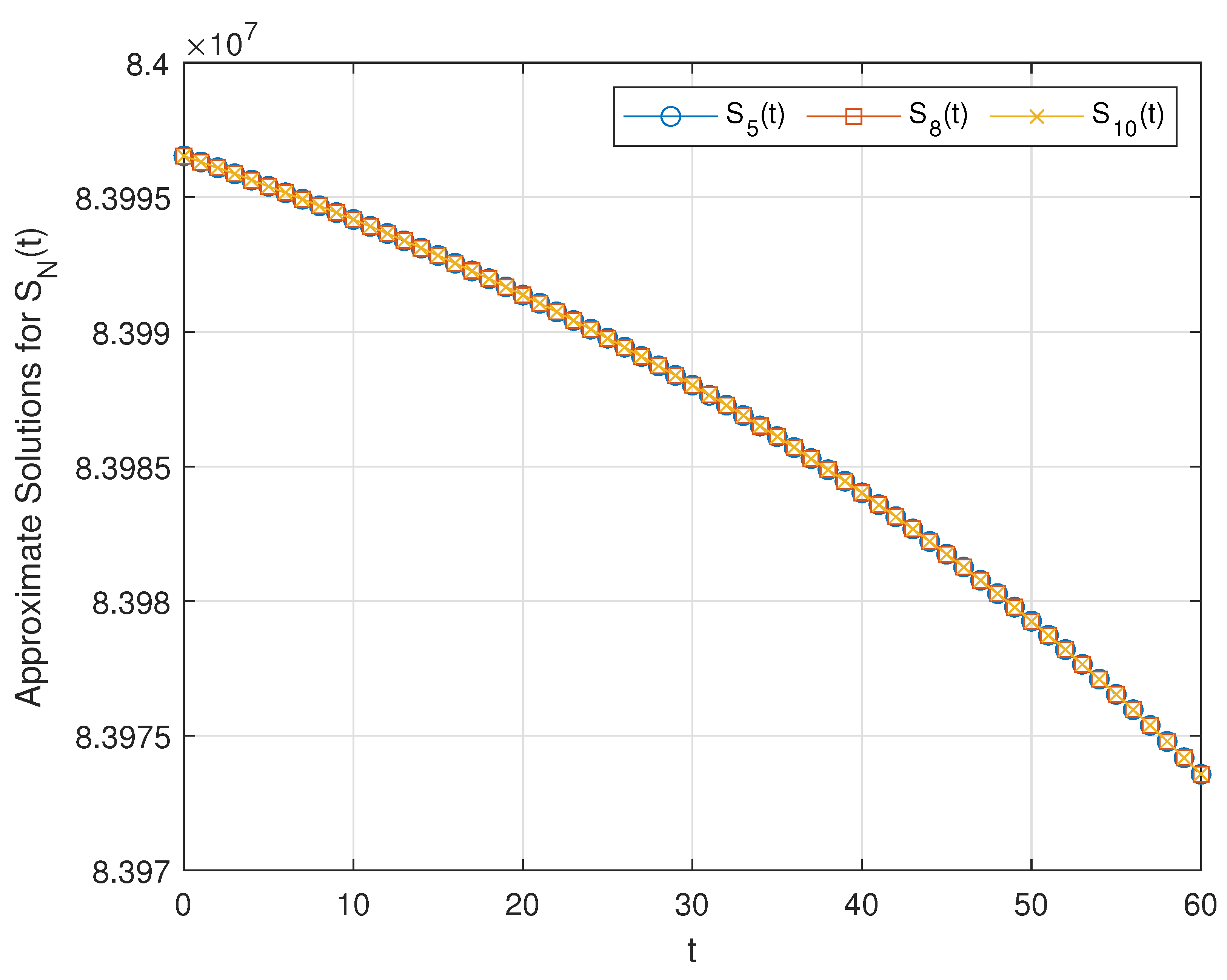
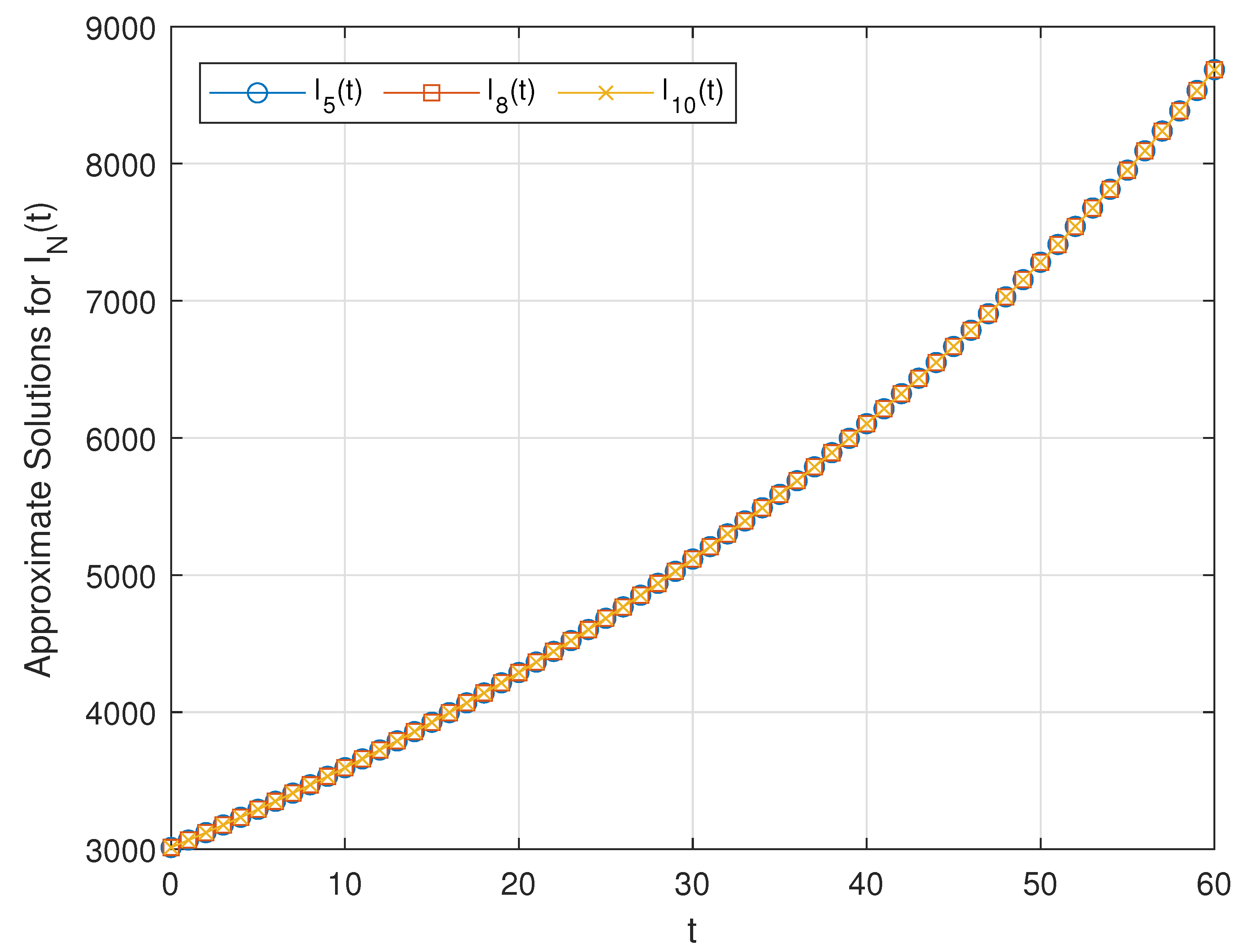
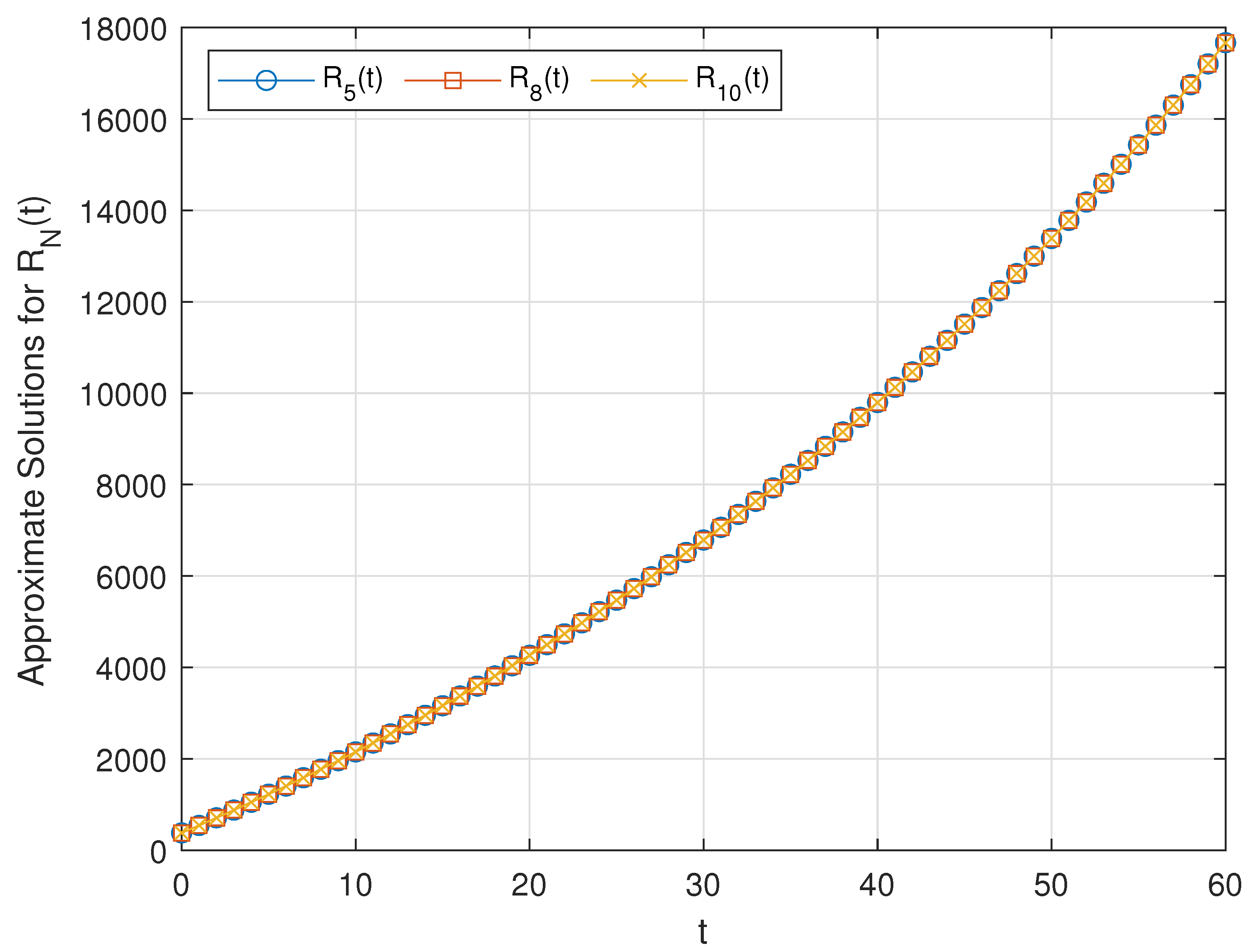
In
Figure 2,
Figure 3 and
Figure 4, we show the Pell–Lucas polynomial solutions
,
,
of the SIR model (
31) for
,
and
. According to this, we interpret that although the susceptible population is decreasing, the infected population and the removed population are increasing. In
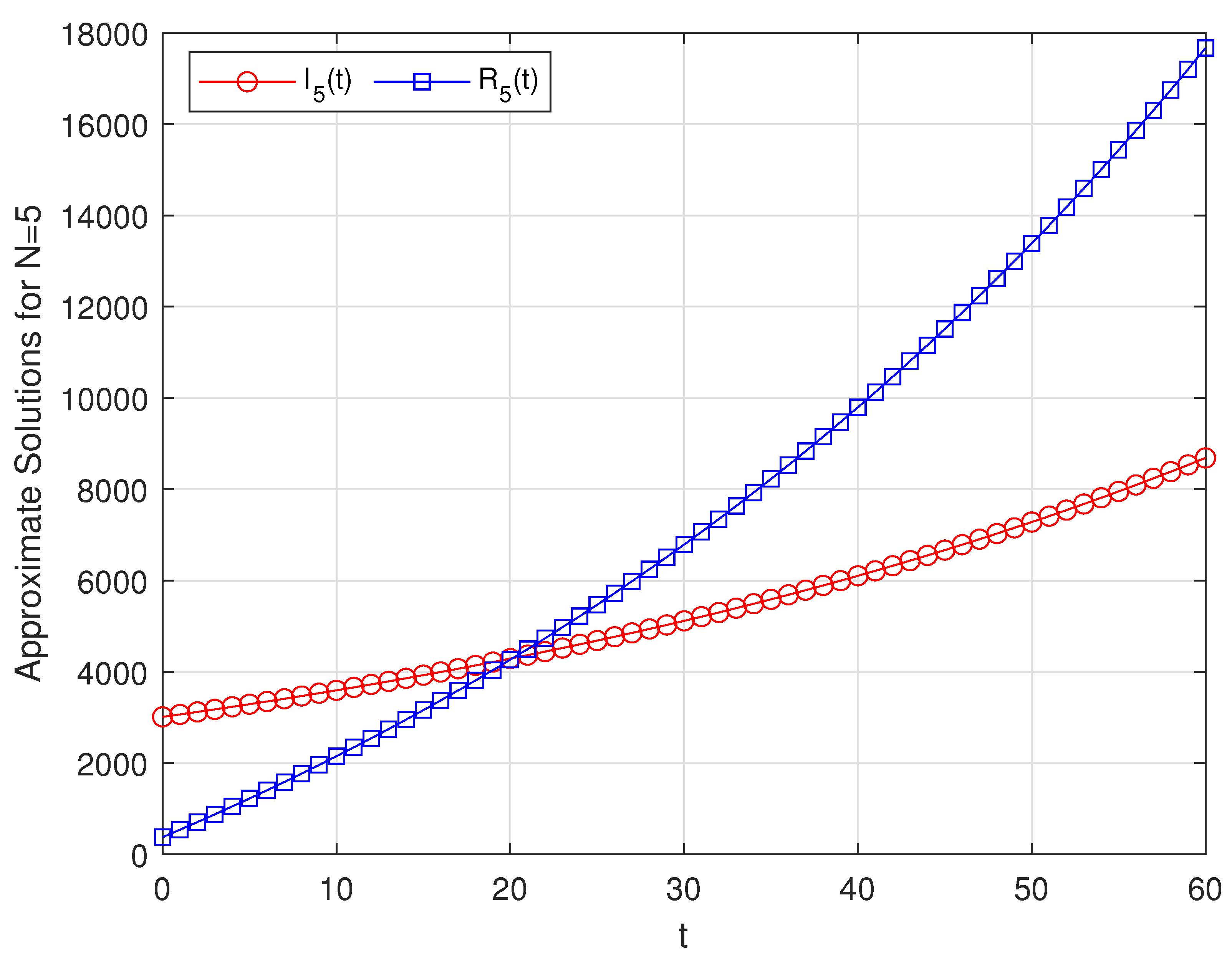
Figure 5, we demonstrate that the Pell–Lucas polynomial solutions
and
of model (
31) for
. From here, we said that the removed population is increased at a greater rate. Accordingly, the removed rate is quite high compared to the infected rate at 60 days. Also, we compare the Pell–Lucas polynomial solutions
,
,
of the SIR model (
31) for
with those of the Runge–Kutta method in
Figure 6. According to
Figure 6, it is said that the graphs of the presented method and the Runge–Kutta method are similar. That is, we observe that the method is accurate and effective.
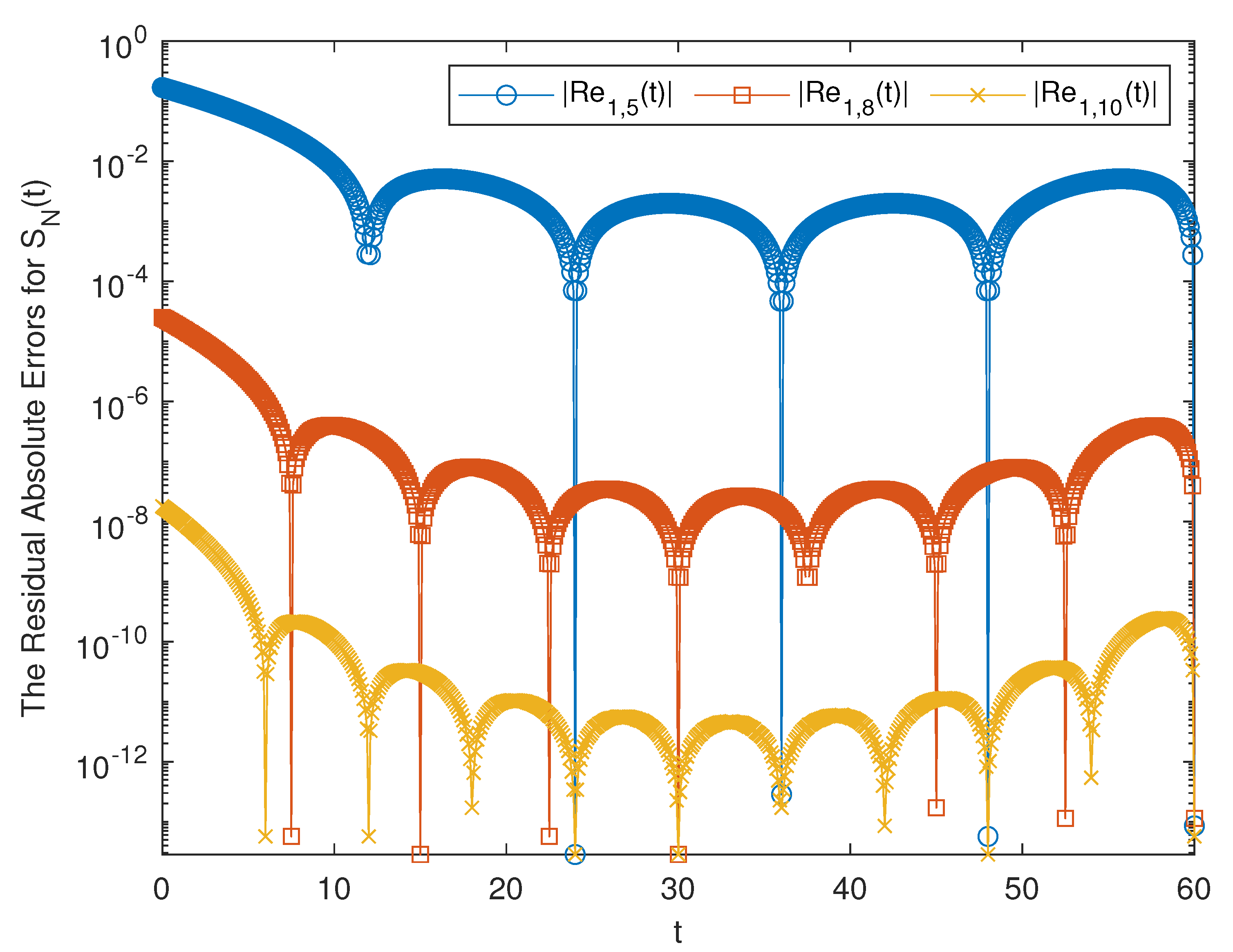
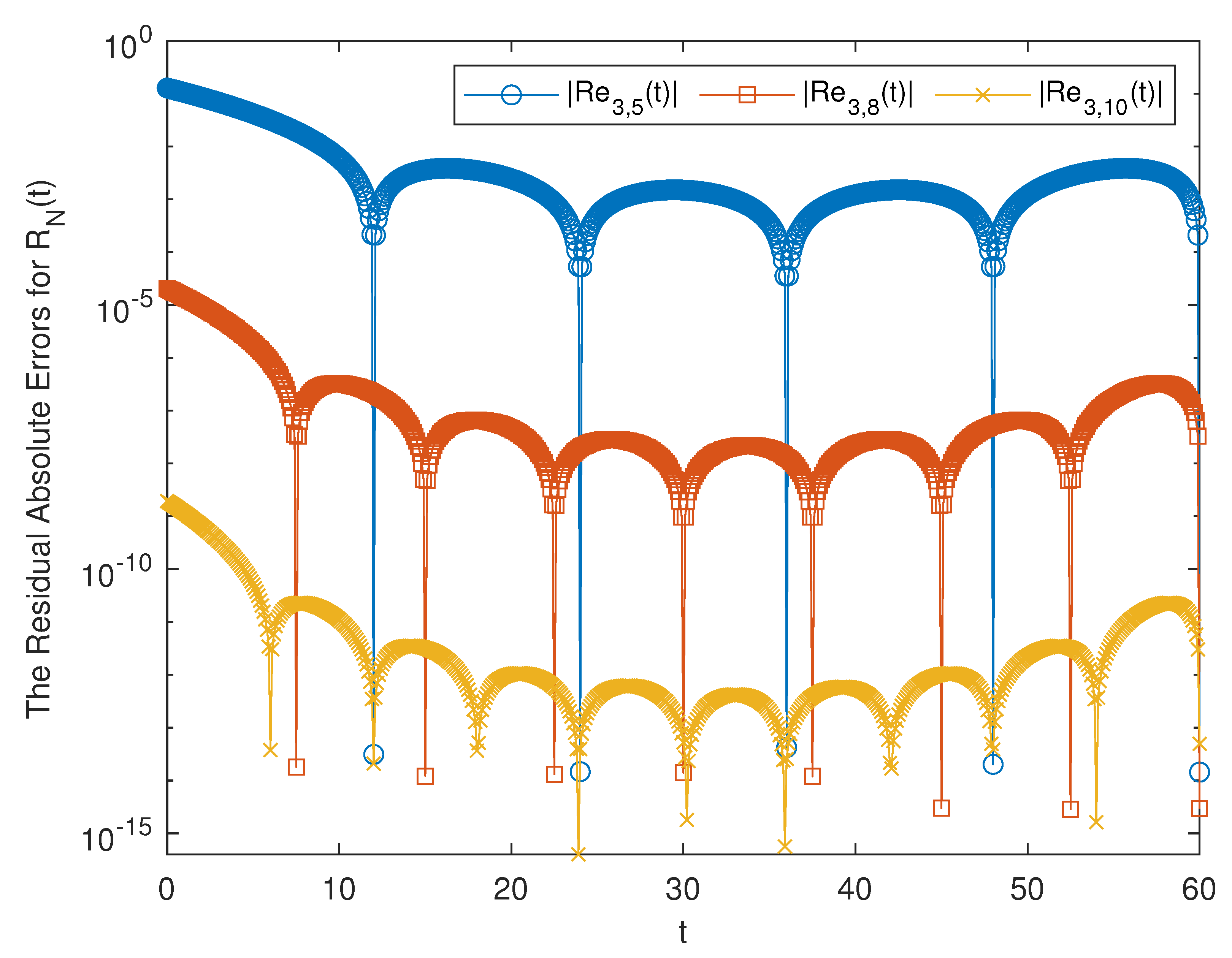
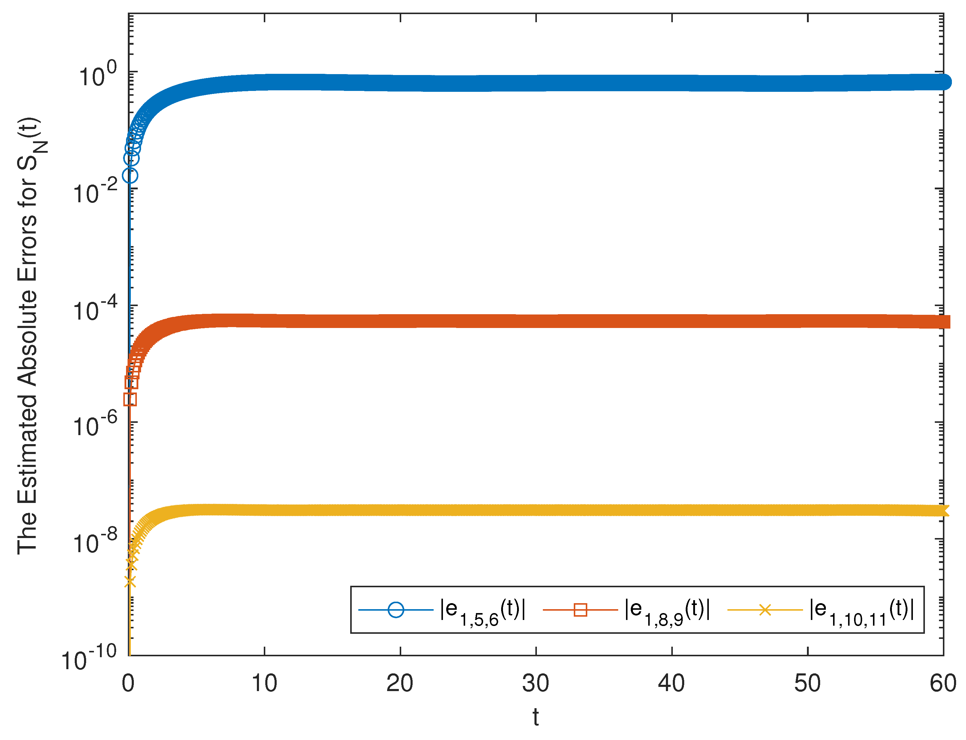
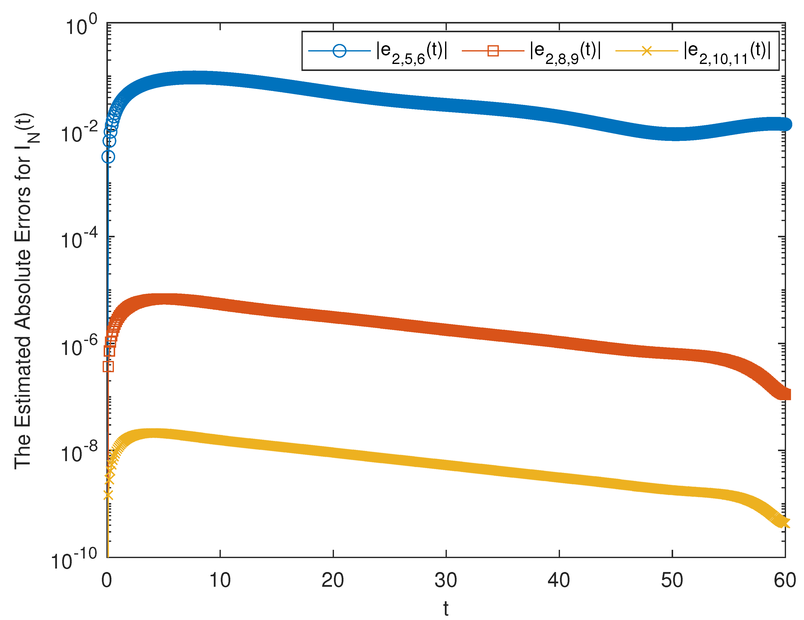
In
Figure 7,
Figure 8 and
Figure 9, we compare the residual absolute error functions of the SIR model (
31) for
,
and
. In addition, we compare the estimated absolute error functions of the SIR model (
31) for
,
and
in
Figure 10,
Figure 11 and
Figure 12. Accordingly, we observe that as the value of
N increases, the errors decrease.
In
Table 4,
Table 5 and
Table 6, we tabulate the residual absolute errors and the estimated absolute errors of the SIR model (
31) for
and
. According to
Table 4,
Table 5 and
Table 6, we observe that as the value of
N increases, the error decreases. Although the residual absolute errors are better than the estimation absolute errors, the estimation absolute errors are not bad either. In other words, the error estimation method presented in
Section 4 give very successful results.
6. Conclusions
This paper proposes a numerical method for an SIR model to investigate the present condition of COVID-19 disease contamination and to estimate its future improvements in Turkey. The parameters and the initial conditions of this model are determined by using real data. The presented method is a collocation approach based on the Pell–Lucas polynomials. According to the Pell–Lucas collocation method, the SIR model is reduced to a system of nonlinear algebraic equations. The solutions of this nonlinear algebraic system determine coefficients of the Pell–Lucas polynomial solutions of the SIR model. Additionally, two error analyses are made. According to
Figure 2,
Figure 3 and
Figure 4, it is interpreted that although the susceptible population is decreasing, the infected population and the removed population are increasing. Also in
Figure 5, it is observed that the removed population increases from 378 to 17,667 for the same value of
N whereas the infected population increases from 3013 to 8685 for
. In the 60-day period from 4 April 2020, an increase in the number of the infected patients is observed. Nevertheless, a faster increase is observed in the number of the removed patients. In that case, we expect that the pandemic will diminish when enough isolation precautions are continued. In
Figure 6, we compare the approximate solutions
,
,
for
with those of the Runge–Kutta method. Accordingly, it is concluded that the graphs obtained from the presented method and the Runge–Kutta method are similar.
In
Figure 7,
Figure 8,
Figure 9,
Figure 10,
Figure 11 and
Figure 12 and
Table 4,
Table 5 and
Table 6, we examine the residual absolute errors and the estimated absolute errors of the approximate solution functions. According to these, we deduce that as the value of
N increases the error decreases. Even though, the residual absolute errors are better than the estimation absolute errors, the estimation absolute errors are not bad either. Accordingly, we comment that the Pell–Lucas collocation method is the effective method to get the approximate solutions of the SIR model. A limitation of the method is that the individuals
in the model represents the number of individuals who both recovered and died. However, the method can be improved by making necessary adjustments to the model. A more important advantage of the method than all these advantages is that the parameters in the model can be determined for different countries, and this method can be developed for other countries as well. Moreover, this method can be developed for similar infections. In the future, in similar epidemic situations, the method can be applied by determining the parameters of the model and the initial conditions in the model. Moreover, the results are obtained in a very short time thanks to the code written in MATLAB. Hereby, the cautious provisions can be made to minimize infections and to intercept an overloading of the health system.


