Investigation of the Stress-Strain State of a Rectangular Plate after a Temperature Shock

Abstract

In this paper, the temperature shock phenomenon is considered. This phenomenon occurs during the operation of engineering structures on Earth and in outer space. A rectangular plate has been selected as a structural element exposed to temperature shock. It has a rigidly sealed edge and three free edges. A one-dimensional third initial boundary value problem of thermal conductivity was posed and solved to study the stress–strain state of the plate. Fourier’s law was used to solve this problem, taking into account the inertial term, since the temperature shock is a fairly fast-dynamic phenomenon. It was believed that all the thermophysical properties of the plate are constant and do not depend on its temperature. As a result, the temperature field of the plate was obtained after the temperature shock. This temperature field generates temperature stresses inside the plate, which lead to temperature deformations. To determine these deformations, the initial boundary value problem of thermoelasticity was posed and solved in this work. The Sophie Germain equation was used while solving this problem. To describe the plate, the theory of flexible plates was used, taking into account the stresses in the middle surface of the plate. Next, the accuracy of analytical solutions for the points displacement of a homogeneous plate subjected to a temperature shock was investigated. The temperature field was constructed using a numerical simulation. Functions of the displacement vector components were obtained using approximate analytical solutions. The accuracy of approximate analytical solutions for the components of the plate points deformation vector was estimated. The obtained results allow us to describe the stress–strain state of the plate after the temperature shock. The results of this work can be used in the design of engineering structures for both terrestrial and space purposes in terms of stability calculations and the implementation of deformation constraints.

1. Introduction

Temperature shock is a fast-dynamic phenomenon that occurs due to the appearance or disappearance of a heat flux [1,2,3]. A striking example of temperature shock in outer space is when a spacecraft enters into the Earth’s shadow or comes out of it [4,5,6]. In this case, large elastic elements experience a temperature shock and undergo temperature deformations. These deformations create disturbances that affect the rotational motion of the spacecraft around the center of mass. This is especially true for small spacecraft [7,8]. When implementing gravity-sensitive technological processes on board small spacecraft, significant restrictions are imposed on micro-accelerations inside the working area of the technological equipment [9,10]. Perturbations from temperature shock can violate these restrictions [11,12]. Therefore, it is important to study temperature shock when designing promising small technological spacecraft.

However, even in terrestrial conditions, individual structural elements can be subjected to temperature shock [13,14,15]. It is important to study temperature shock when exploring the stability of structures [16,17,18], as well as to check the fulfillment of restrictions on the magnitude of the deformation [19,20,21]. In this paper, a homogeneous rectangular plate is considered as one of the most common structural elements.

It is important to study temperature shock when designing various structural elements that are subjected to temperature differences. In [22], the material resistance to temperature shock is investigated, the need to protect structures from temperature shock is noted and a number of stability criteria are obtained. The authors of the work [23] indicate the degradation of ceramic materials as a result of temperature shock. Work [24] is devoted to modeling the behavior of a functionally profiled metal–ceramic plate subjected to temperature shock in a nuclear reactor. The works [25,26] are devoted to measurements of temperature shock parameters in metals and porous reinforced materials. The works [27,28] are devoted to the memory effect during temperature shock. In [29,30], thermal oscillations under a laser are investigated. Works [31,32] contain the results of the stress after welding studies.

Temperature shock plays an important role in the development of laws for controlling spacecraft with movement of large elastic elements. Solar panels, external radiator panels, antennas and other structural elements of the spacecraft usually act as large elastic elements. When a spacecraft moves along its orbit, it enters into the Earth’s shadow and comes out of it. In this event, temperature shock of large elastic elements occurs. In [33], a significant influence of temperature shock on spacecraft dynamics is noted. Works [19,34] are devoted to the large elastic elements vibrations resulting from temperature shock. The authors of [6,7,11] note that temperature shock especially affects the dynamics of the rotational motion of small spacecraft. It should also be noted that there is a temperature shock effect on gravity-sensitive processes on board the spacecraft. This information can be found in [18,35].

In this paper, a new approximate analytical solution to the thermoelasticity problem is obtained, which corresponds to the third initial boundary value problem of one-dimensional thermal conductivity. An analysis of the applicability of this solution in the stress–strain state of large elastic elements of spacecraft under temperature shock was carried out. The possibility of using this solution in estimating the displacement vector of the small spacecraft solar panel points is shown. Displacements are considered within temperature shock. The obtained approximate analytical solution is important for estimating micro-accelerations arising from temperature shock. It can be used in the design of small technological spacecraft to verify that the requirements for micro-accelerations during the implementation of gravity-sensitive processes on board are satisfied [9,36]. The computational experiment was carried out under the conditions of space that is near to Earth.

2. One-Dimensional Third Initial Boundary Value Problem of Thermal Conductivity

A homogeneous rectangular plate with constant thermophysical properties was subjected to temperature shock. Moreover, at the time of the temperature shock, it had a flat shape and was not deformed (the dotted line in Figure 1).

In this case, with a homogeneous and stationary heat flux, it can be assumed that the surface layer of the plate was heated by this flux uniformly. Thus, the temperature of all points of the surface layer in the first approximation can be considered the same. The initial temperature field of the plate is considered a homogeneous field with the same temperature, T₀, at all points on the plate. In this formulation, a one-dimensional model of thermal conductivity is valid, in which temperature is a function of only one spatial coordinate and time: $T=T(z,\hspace{0.17em}\hspace{0.17em}t)$. A one-dimensional thermal conductivity equation was used for such a model, assuming that the heat fluxes inside the plate propagate only in the direction of the z-axis:

$$\frac{\partial T(z,\hspace{0.17em}\hspace{0.17em}t)}{\partial t}=a^2\frac{{\partial }^{2}T(z,\hspace{0.17em}\hspace{0.17em}t)}{\partial z^2},\hspace{0.17em}\hspace{0.17em}-\frac{h}{2}\le z\le \frac{h}{2},\hspace{0.17em}\hspace{0.17em}t>0$$

(1)

where a is the coefficient of thermal conductivity and h is the thickness of the plate.

To formulate the third initial boundary value problem, we supplemented the heat Equation (1) with boundary conditions of a third kind:

$$\lambda \frac{\partial T\left(-\frac{h}{2},\hspace{0.17em}\hspace{0.17em}t\right)}{\partial z}=-e\mathrm{\Theta }\left[T{\left(-\frac{h}{2},\hspace{0.17em}\hspace{0.17em}t\right)}^4-T_c^4\right],\hspace{0.17em}\hspace{0.17em}z=-\frac{h}{2},\hspace{0.17em}\hspace{0.17em}t>0$$

(2)

where λ is the coefficient of thermal conductivity, e is the degree of blackness of the plate material, Θ is the Stefan-Boltzmann constant and T_c is the temperature of the environment surrounding the plate.

$$\lambda \frac{\partial T\left(\frac{h}{2},\hspace{0.17em}\hspace{0.17em}t\right)}{\partial z}=Q-e\mathrm{\Theta }\left[T{\left(\frac{h}{2},\hspace{0.17em}\hspace{0.17em}t\right)}^4-T_c^4\right],\hspace{0.17em}\hspace{0.17em}z=\frac{h}{2},\hspace{0.17em}\hspace{0.17em}t>0$$

(3)

where Q is the heat flux incident on the surface layer of the plate.

We supplemented the task with the initial conditions:

$$T(z,\hspace{0.17em}\hspace{0.17em}0)=T_0,\hspace{0.17em}\hspace{0.17em}-\frac{h}{2}\le z\le \frac{h}{2},\hspace{0.17em}\hspace{0.17em}t=0$$

(4)

where T₀ is an initial temperature, equal for all points on the plate.

Thus, the system (1)–(4) represents the third initial boundary value problem with a one-dimensional equation of thermal conductivity. The result is a dynamic temperature field of the plate points. The third initial boundary value problem can be solved only by numerical methods [37,38] since the boundary conditions of the third kind (2) and (3) were essentially nonlinear.

3. The Problem of Thermoelasticity

We considered the stress–strain state of the plate that caused this temperature field after determining the dynamic temperature field $T=T(z,\hspace{0.17em}\hspace{0.17em}t)$ from the initial boundary value problem (1)–(4). We used the vector $\overrightarrow{\Delta }\left(u,\hspace{0.17em}\hspace{0.17em}v,\hspace{0.17em}\hspace{0.17em}w\right)$ to determine the displacement of the plate points. We assumed, as a first approximation, that the changes in the coordinate points along the x-axis (Figure 1) were negligible compared to the changes in other coordinates, i.e., u = 0. In accordance with the one-dimensional model of thermal conductivity (1)–(4), we assumed that the deflection of the plate points was a function of only the longitudinal coordinate and time: $w=w(x,\hspace{0.17em}\hspace{0.17em}t)$. The Sophie Germain equation with an inertial term determined the deflection of the plate in the direction of the z-axis [5]:

$$D\frac{{\partial }^{4}w(x,\hspace{0.17em}\hspace{0.17em}t)}{\partial x^4}+\rho \hspace{0.17em}h\frac{{\partial }^{2}w(x,\hspace{0.17em}\hspace{0.17em}t)}{\partial t^2}=-2\mu \alpha {\displaystyle \underset{h/2}{\overset{-h/2}{\int }}\left[2\frac{\partial T(z,\hspace{0.17em}\hspace{0.17em}t)}{\partial z}+z\frac{{\partial }^{2}T(z,\hspace{0.17em}\hspace{0.17em}t)}{\partial z^2}\right]}dz,\hspace{0.17em}\hspace{0.17em}0\le x\le l,\hspace{0.17em}\hspace{0.17em}t>0$$

(5)

where D is the cylindrical bending stiffness of the plate, ρ is the density of the plate material, μ is the Lame coefficient, α is the coefficient of linear expansion of the plate material and l is the length of the plate.

In fact, Equation (5) describes the deflection of the median surface of the plate under the assumption that it is thin.

Equation (5) was supplemented with boundary conditions.

Geometric boundary conditions with fixed edges (hard sealing conditions):

$$\{\begin{array}{l}\hspace{0.17em}w\left(0,\hspace{0.17em}\hspace{0.17em}t\right)=0,\hspace{0.17em}\hspace{0.17em}x=0,\hspace{0.17em}\hspace{0.17em}t>0;\\ \frac{\partial w\left(x,\hspace{0.17em}\hspace{0.17em}t\right)}{\partial x}=0,\hspace{0.17em}\hspace{0.17em}x=0,\hspace{0.17em}\hspace{0.17em}t>0.\end{array}$$

(6)

Free edge static boundary conditions:

$$\{\begin{array}{l}\hspace{0.17em}\frac{{\partial }^{2}w\left(x,\hspace{0.17em}\hspace{0.17em}t\right)}{\partial x^2}+\nu \frac{{\partial }^{2}w\left(x,\hspace{0.17em}\hspace{0.17em}t\right)}{\partial y^2}=0,\hspace{0.17em}\hspace{0.17em}x=l,\hspace{0.17em}\hspace{0.17em}t>0;\\ \frac{{\partial }^{3}w\left(x,\hspace{0.17em}\hspace{0.17em}t\right)}{\partial x^3}+\left(2-\nu \right)\frac{{\partial }^{3}w\left(x,\hspace{0.17em}\hspace{0.17em}t\right)}{\partial x\hspace{0.17em}\partial y^2}=0,\hspace{0.17em}\hspace{0.17em}x=l,\hspace{0.17em}\hspace{0.17em}t>0,\end{array}$$

(7)

where ν is the Poisson’s ratio.

Since the deflection did not depend on the transverse y coordinate, the boundary conditions (7) were significantly simplified:

$$\{\begin{array}{l}\hspace{0.17em}\frac{{\partial }^{2}w\left(x,\hspace{0.17em}\hspace{0.17em}t\right)}{\partial x^2}=0,\hspace{0.17em}\hspace{0.17em}x=l,\hspace{0.17em}\hspace{0.17em}t>0;\\ \frac{{\partial }^{3}w\left(x,\hspace{0.17em}\hspace{0.17em}t\right)}{\partial x^3}=0,\hspace{0.17em}\hspace{0.17em}x=l,\hspace{0.17em}\hspace{0.17em}t>0.\end{array}$$

(8)

Equation (5) was supplemented with the initial conditions, taking into account the fact that, at the initial moment, the plate was not deformed:

$$w(x,\hspace{0.17em}\hspace{0.17em}0)=0,\hspace{0.17em}\hspace{0.17em}0\le x\le l,\hspace{0.17em}\hspace{0.17em}\hspace{0.17em}t=0$$

(9)

It was proposed that the following polynomial be considered to obtain a solution to the initial boundary value problem (5), (6), (8), (9):

$$w(x,\hspace{0.17em}\hspace{0.17em}t)=\frac{t}{t+a}\left(A{x}^4+B{x}^3+C{x}^2\right),\hspace{0.17em}\hspace{0.17em}0\le x\le l,\hspace{0.17em}\hspace{0.17em}\hspace{0.17em}t>0$$

(10)

where a > 0 is a positive constant; A, B and C are also constants.

The following expression was obtained as a result of the well-known method [39,40] of representing a function of two variables as a product: $w(x,\hspace{0.17em}\hspace{0.17em}t)=X(x)T(t),\hspace{0.17em}\hspace{0.17em}0\le x\le l,\hspace{0.17em}\hspace{0.17em}\hspace{0.17em}t>0$. The first factor in the expression (10) $\frac{t}{t+a}$ ensured that the initial conditions were fulfilled (9). The constants A, B and C of the polynomial were selected based on the boundary conditions (6) and (8):

$$\{\begin{array}{l}\hspace{0.17em}\frac{t}{t+a}\left(12A{x}^2+6Bx+2C\right)=0,\hspace{0.17em}\hspace{0.17em}x=l,\hspace{0.17em}\hspace{0.17em}t>0;\\ \frac{t}{t+a}\left(24Ax+6B\right)=0,\hspace{0.17em}\hspace{0.17em}x=l,\hspace{0.17em}\hspace{0.17em}t>0.\end{array}$$

(11)

From which:

$$\{\begin{array}{l}\hspace{0.17em}C=6A{l}^2;\\ B=-4Al.\end{array}$$

(12)

Thus, (10) is converted into the following expression:

$$w(x,\hspace{0.17em}\hspace{0.17em}t)=\frac{At}{t+a}\left(x^4-4l{x}^3+6l^2{x}^2\right),\hspace{0.17em}\hspace{0.17em}0\le x\le l,\hspace{0.17em}\hspace{0.17em}\hspace{0.17em}t>0$$

(13)

Substituting solution (13) into Equation (5) shows the correspondence to the simulated situation:

$$12D\hspace{0.17em}\cdot A\frac{t}{t+a}-A\frac{a\rho \hspace{0.17em}h}{{\left(t+a\right)}^3}\left(x^4-4l{x}^3+6l^2{x}^2\right)=-\mu \alpha {\displaystyle \underset{-h/2}{\overset{h/2}{\int }}\left[2\frac{\partial T(z,\hspace{0.17em}\hspace{0.17em}t)}{\partial z}+z\frac{{\partial }^{2}T(z,\hspace{0.17em}\hspace{0.17em}t)}{\partial z^2}\right]}dz,\hspace{0.17em}\hspace{0.17em}0\le x\le l,\hspace{0.17em}\hspace{0.17em}t>0$$

(14)

Equation (14) contained two parameters (a and A) that could be varied to satisfy it. In the case where Equation (14) was not satisfied under any parameters when substituting the temperature field, it was necessary to look for a polynomial different from (13).

We further considered another component of the displacement vector $\overrightarrow{\Delta }\left(u,\hspace{0.17em}\hspace{0.17em}v,\hspace{0.17em}\hspace{0.17em}w\right)$. Due to the symmetry of the problem in relation to the longitudinal x-axis of the plate, there were reasons to believe that its movement in the direction of the y-axis would also be symmetrical. At the same time, these movements depended on the longitudinal and transverse coordinates: $v=v(x,\hspace{0.17em}\hspace{0.17em}y,\hspace{0.17em}\hspace{0.17em}t)$. Therefore, we considered only half of the plate: $0\le y\le \frac{b}{2}$. We supposed that, after the temperature shock, the plate came to an equilibrium state in which its movements could be neglected. Thus, the equilibrium equation would be valid, considering that the plate was isotropic [38]:

$$\frac{3(1-\nu )}{1+\nu }grad\hspace{0.17em}\hspace{0.17em}div\hspace{0.17em}\hspace{0.17em}\overrightarrow{\Delta }\hspace{0.17em}\hspace{0.17em}-\hspace{0.17em}\hspace{0.17em}\frac{3(1-2\nu )}{2\left(1+\nu \right)}\hspace{0.17em}\hspace{0.17em}rot\hspace{0.17em}\hspace{0.17em}rot\hspace{0.17em}\hspace{0.17em}\overrightarrow{\Delta }=\alpha \hspace{0.17em}\hspace{0.17em}grad\hspace{0.17em}\hspace{0.17em}T,\hspace{0.17em}\hspace{0.17em}\hspace{0.17em}t=\infty$$

(15)

In (15) and further, the moment of the equilibrium state onset was conventionally designated as $t=\infty$. The assumptions introduced earlier allowed us to represent Equation (15) in scalar form:

$$\{\begin{array}{l}\hspace{0.17em}\frac{{\partial }^{2}v\left(x,\hspace{0.17em}\hspace{0.17em}y,\hspace{0.17em}\hspace{0.17em}t\right)}{\partial x\hspace{0.17em}\partial y}=0,\hspace{0.17em}\hspace{0.17em}\hspace{0.17em}0\le x\le l,\hspace{0.17em}\hspace{0.17em}0\le y\le \frac{b}{2},\hspace{0.17em}\hspace{0.17em}\hspace{0.17em}t=\infty ;\\ \frac{3\left(1-\nu \right)}{1+\nu }\frac{{\partial }^{2}v\left(x,\hspace{0.17em}\hspace{0.17em}y,\hspace{0.17em}\hspace{0.17em}t\right)}{\partial y^2}+\frac{3\left(1-2\nu \right)}{2\left(1+\nu \right)}\frac{{\partial }^{2}v\left(x,\hspace{0.17em}\hspace{0.17em}y,\hspace{0.17em}\hspace{0.17em}t\right)}{\partial x^2}=0,\hspace{0.17em}\hspace{0.17em}0\le x\le l,\hspace{0.17em}\hspace{0.17em}0\le y\le \frac{b}{2},\hspace{0.17em}\hspace{0.17em}\hspace{0.17em}\hspace{0.17em}t=\infty ;\\ \frac{3\left(1-2\nu \right)}{2\left(1+\nu \right)}\frac{{\partial }^{2}w\left(x,\hspace{0.17em}\hspace{0.17em}t\right)}{\partial x^2}=\alpha \hspace{0.17em}\frac{\partial T\left(z,\hspace{0.17em}\hspace{0.17em}t\right)}{\partial z},\hspace{0.17em}\hspace{0.17em}\hspace{0.17em}0\le x\le l,\hspace{0.17em}\hspace{0.17em}0\le y\le \frac{b}{2},\hspace{0.17em}\hspace{0.17em}t=\infty .\end{array}$$

(16)

System (16) could be used as additional end conditions, assuming the equilibrium state of the plate.

On the other hand, inertia forces had to be added to the system (16) to describe the change dynamics in the displacement vector of the plate points $\overrightarrow{\Delta }\left(u,\hspace{0.17em}\hspace{0.17em}v,\hspace{0.17em}\hspace{0.17em}w\right)$. Previously, it was assumed that u = 0. Therefore, the first Equation (16) was valid for t > 0. This meant that the movement of the plate pointed in the direction of the y-axis could be represented as the sum of two independent functions:

$$v\left(x,\hspace{0.17em}\hspace{0.17em}y,\hspace{0.17em}\hspace{0.17em}t\right)=v_1\left(x,\hspace{0.17em}\hspace{0.17em}t\right)+v_2\left(y,\hspace{0.17em}\hspace{0.17em}t\right)$$

(17)

As for the third Equation (16), if the assumptions made were correct, this meant it was necessary to impose additional restrictions on the function $T=T(z,\hspace{0.17em}\hspace{0.17em}t)$. This may have depended on z only linearly. In this case, the derivative $\frac{\partial T(z,\hspace{0.17em}\hspace{0.17em}t)}{\partial z}$ did not depend on z. This did not conflict with the assumption that $w=w(x,\hspace{0.17em}\hspace{0.17em}t)$. Using this equation with such a restriction was difficult. However, to determine the deflection, the Sophie Germain Equation (5) was used, which was free from the specified restriction. Both the first and second partial derivatives in this case could depend on z in any way. Thus, the second Equation (16) was of interest. The values $\frac{{\partial }^{2}v(x,\hspace{0.17em}\hspace{0.17em}y,\hspace{0.17em}\hspace{0.17em}t)}{\partial x^2}$ and $\frac{{\partial }^{2}v(x,\hspace{0.17em}\hspace{0.17em}y,\hspace{0.17em}\hspace{0.17em}t)}{\partial y^2}$ represented, in the first approximation, the curvature of the deformed plate in the direction of the x- and y-axes, respectively. Based on the assumptions made, it could be concluded that the segments of the plate parallel to the y-axis would remain rectilinear after deformation. This made it possible to assert that $\frac{{\partial }^{2}v(x,\hspace{0.17em}\hspace{0.17em}y,\hspace{0.17em}\hspace{0.17em}t)}{\partial y^2}=0$ and rewrite (17) in the form:

$$v\left(x,\hspace{0.17em}\hspace{0.17em}y,\hspace{0.17em}\hspace{0.17em}t\right)=v_1\left(x,\hspace{0.17em}\hspace{0.17em}t\right)+y\hspace{0.17em}{v}_3\left(\hspace{0.17em}t\right)$$

(18)

Then, taking into account the inertial term for an infinitesimal strip of plate with $h\frac{b}{2}dx$ volume, the second Equation (16) has the form:

$$\begin{array}{l}D\frac{3\left(1-2\nu \right)}{2\left(1+\nu \right)}\frac{{\partial }^{3}v\left(x,y,\hspace{0.17em}\hspace{0.17em}t\right)}{\partial x^3}dx+\rho \frac{{\partial }^{2}v\left(x,y,\hspace{0.17em}\hspace{0.17em}t\right)}{\partial t^2}h\frac{b}{2}dx=E\alpha \hspace{0.17em}dx{\displaystyle \underset{-h/2}{\overset{h/2}{\int }}\left[T\left(z,\hspace{0.17em}\hspace{0.17em}t\right)-T_0\right]}\hspace{0.17em}dz,\hspace{0.17em}\hspace{0.17em}\hspace{0.17em}\hspace{0.17em}\\ 0\le x\le l,\hspace{0.17em}\hspace{0.17em}0\le y\le \frac{b}{2},\hspace{0.17em}\hspace{0.17em}t>0\end{array}$$

(19)

We supposed that $\frac{{\partial }^2{v}_1(x,\hspace{0.17em}\hspace{0.17em}t)}{\partial t^2}>>\frac{d^2{v}_3(\hspace{0.17em}t)}{d{t}^2}$. Then, taking into account the decomposition, we got (18):

$$\frac{3\left(1-2\nu \right)}{2\left(1+\nu \right)}\frac{{\partial }^3{v}_1\left(x,t\right)}{\partial x^3}+\frac{6\rho \left(1-{\nu }^2\right)}{E{h}^2}\frac{{\partial }^2{v}_1\left(x,\hspace{0.17em}t\right)}{\partial t^2}b=\frac{12\left(1-{\nu }^2\right)}{h^3}\alpha {\displaystyle \underset{-h/2}{\overset{h/2}{\int }}\left[T\left(z,\hspace{0.17em}\hspace{0.17em}t\right)-T_0\right]}\hspace{0.17em}dz,\hspace{0.17em}\hspace{0.17em}0\le x\le l,\hspace{0.17em}\hspace{0.17em}t>0$$

(20)

where E is Young’s modulus.

Equation (20) could be considered as the equation of the first approximation for determining the component of the displacement vector $v=v(x,\hspace{0.17em}\hspace{0.17em}y,\hspace{0.17em}\hspace{0.17em}t)$ taking into account (18). We supplemented (20) with boundary conditions.

Geometric boundary conditions with fixed edges (hard sealing conditions):

$$\{\begin{array}{l}\hspace{0.17em}v\left(0,y,\hspace{0.17em}\hspace{0.17em}t\right)=0,\hspace{0.17em}\hspace{0.17em}x=0,\hspace{0.17em}\hspace{0.17em}0\le y\le \frac{b}{2},\hspace{0.17em}\hspace{0.17em}t>0;\\ \frac{\partial v\left(x,\hspace{0.17em}\hspace{0.17em}y,\hspace{0.17em}\hspace{0.17em}t\right)}{\partial x}=0,\hspace{0.17em}\hspace{0.17em}x=0,\hspace{0.17em}\hspace{0.17em}0\le y\le \frac{b}{2},\hspace{0.17em}\hspace{0.17em}t>0.\end{array}$$

(21)

Taking into account the decomposition (18), we transformed (21):

$$\{\begin{array}{l}\hspace{0.17em}{v}_1\left(0,\hspace{0.17em}\hspace{0.17em}t\right)=-\frac{b}{2}\hspace{0.17em}{v}_3(t),\hspace{0.17em}\hspace{0.17em}x=0,\hspace{0.17em}\hspace{0.17em}y=\frac{b}{2},\hspace{0.17em}\hspace{0.17em}t>0;\\ \frac{\partial v_1\left(x,\hspace{0.17em}\hspace{0.17em}t\right)}{\partial x}=0,\hspace{0.17em}\hspace{0.17em}x=0,\hspace{0.17em}\hspace{0.17em}t>0.\end{array}$$

(22)

Free edge x = l static boundary conditions:

$$\{\begin{array}{l}\hspace{0.17em}\frac{{\partial }^2{v}_1\left(x,\hspace{0.17em}\hspace{0.17em}t\right)}{\partial x^2}+\nu \frac{{\partial }^{2}v\left(x,\hspace{0.17em}\hspace{0.17em}t\right)}{\partial y^2}=0,\hspace{0.17em}\hspace{0.17em}x=l,\hspace{0.17em}\hspace{0.17em}t>0;\\ \frac{{\partial }^{3}v\left(x,\hspace{0.17em}\hspace{0.17em}t\right)}{\partial x^3}+\left(2-\nu \right)\frac{{\partial }^{3}v\left(x,\hspace{0.17em}\hspace{0.17em}t\right)}{\partial x\hspace{0.17em}\partial y^2}=0,\hspace{0.17em}\hspace{0.17em}x=l,\hspace{0.17em}\hspace{0.17em}t>0,\end{array}$$

(23)

Taking into account the decomposition (18), we transformed (23):

$$\{\begin{array}{l}\hspace{0.17em}\frac{{\partial }^2{v}_1\left(x,\hspace{0.17em}\hspace{0.17em}t\right)}{\partial x^2}=0,\hspace{0.17em}\hspace{0.17em}x=l,\hspace{0.17em}\hspace{0.17em}t>0;\\ \frac{{\partial }^3{v}_1\left(x,\hspace{0.17em}\hspace{0.17em}t\right)}{\partial x^3}=0,\hspace{0.17em}\hspace{0.17em}x=l,\hspace{0.17em}\hspace{0.17em}t>0,\end{array}$$

(24)

We supplemented Equation (20) with the initial conditions characterizing the absence of the initial deformations of the plate:

$$v(x,\hspace{0.17em}\hspace{0.17em}y,\hspace{0.17em}\hspace{0.17em}0)=0,\hspace{0.17em}\hspace{0.17em}0\le x\le l,\hspace{0.17em}\hspace{0.17em}\hspace{0.17em}0\le y\le \frac{b}{2},\hspace{0.17em}\hspace{0.17em}t=0$$

(25)

As a solution, the following function was selected:

$$v_1(x,\hspace{0.17em}\hspace{0.17em}t)=-\alpha \frac{b}{2}\left[T\left(0,\hspace{0.17em}\hspace{0.17em}t\right)-T_0\right]{\left(1-\frac{x^2}{l^2}\right)}^4,\hspace{0.17em}\hspace{0.17em}0\le x\le l,\hspace{0.17em}\hspace{0.17em}\hspace{0.17em}t>0$$

(26)

It was easy to verify that function (26) satisfies the second Equation (22) and both Equation (24). Then, from the first Equation (22), we obtained:

$$v_3(t)=\alpha \left[T\left(0,\hspace{0.17em}\hspace{0.17em}t\right)-T_0\right],\hspace{0.17em}\hspace{0.17em}\hspace{0.17em}t>0$$

(27)

In this case, decomposition (18) took the form:

$$v\left(x,\hspace{0.17em}\hspace{0.17em}y,\hspace{0.17em}\hspace{0.17em}t\right)=\alpha \left[T\left(0,\hspace{0.17em}\hspace{0.17em}t\right)-T_0\right]\left[y-\frac{b}{2}{\left(1-\frac{x^2}{l^2}\right)}^4\right],\hspace{0.17em}\hspace{0.17em}0\le x\le l,\hspace{0.17em}\hspace{0.17em}0\le y\le \frac{b}{2},\hspace{0.17em}\hspace{0.17em}t>0$$

(28)

Substituting solution (28) into Equation (20) showed the correspondence to the simulated situation:

$$\begin{array}{l}b\left(1-\frac{x^2}{l^2}\right)\left\{\frac{12x}{l^4}\frac{1-2\nu }{1+\nu }\left[T\left(0,\hspace{0.17em}\hspace{0.17em}t\right)-T_0\right]\left(7\frac{x^2}{l^2}-3\right)-\frac{\rho \left(1-{\nu }^2\right)}{E{h}^2}b{\left(1-\frac{x^2}{l^2}\right)}^3\frac{{\partial }^{2}T\left(0,\hspace{0.17em}t\right)}{\partial t^2}\right\}=\\ =4\frac{1-{\nu }^2}{h^3}{\displaystyle \underset{-h/2}{\overset{h/2}{\int }}\left[T\left(z,\hspace{0.17em}\hspace{0.17em}t\right)-T_0\right]}\hspace{0.17em}dz,\hspace{0.17em}\hspace{0.17em}0\le x\le l,\hspace{0.17em}\hspace{0.17em}t>0\end{array}$$

(29)

However, unlike (14), the parameters of Equation (29) were the mass–dimensional characteristics of the plate. In the case when Equation (29) was not satisfied when substituting the temperature field, it was necessary to look for a solution different from (28).

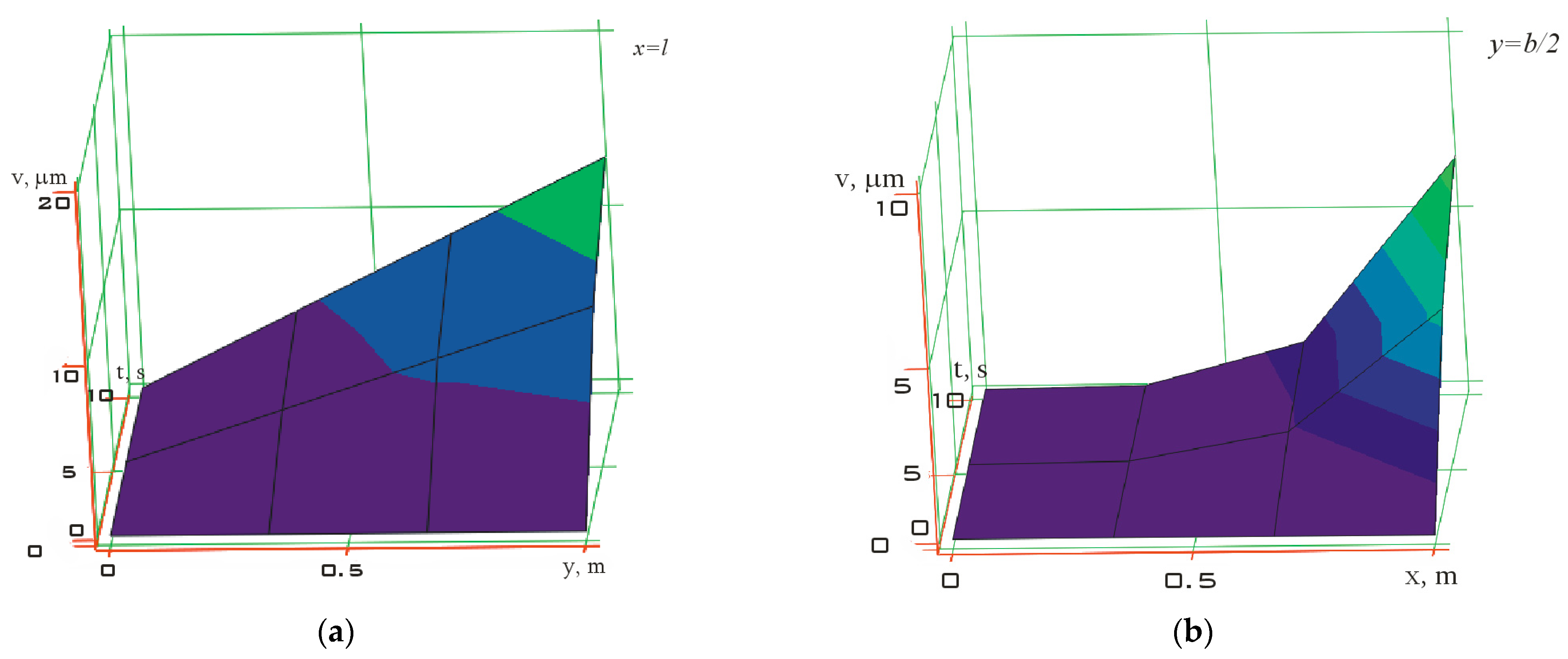
4. Numerical Modeling

We chose the main parameters of the plate corresponding to the work [11] for numerical modeling. In this case, it was possible to compare the results with the data obtained in the ANSYS package. The main characteristics of the simulated plate are given in

Table 1. The main parameters of the simulated plate.

Parameter	Designation	Value	Dimension
Solar panel frame material	–	MA2	–
Coefficient of thermal conductivity	$\lambda$	96.3	W/(m·K)
Stefan-Boltzmann constant	Θ	5.67 × 10−8	W/(m2·K4)
External heat flux	$Q$	1400	W/m2
Vacuum temperature	$T_C$	3	K
Initial temperature of the solar panel frame	$T_0=T(z,\hspace{0.17em}\hspace{0.17em}0)$	200	K
Degree of blackness	e	0.2	-
Specific heat	c	1130.4	J/(kg·K)
Density	$\rho$	1780	kg/m3
Young’s Module	E	4 × 1010	Pa
Shift modulus	μ	1.6 × 1010	Pa
Poisson’s Ratio	ν	0.3	-
Solar panel length	l	1	m
Solar panel width	b	0.5	m
Solar panel frame thickness	h	1	mm

.

For convenient calculations, we combined the coordinate plane xy so that the illuminated surface of the plate had the coordinate x = 0. To simplify expression (14), we assumed in the first approximation that the temperature linearly $T=T(z,\hspace{0.17em}\hspace{0.17em}t)$ depends on z:

$$T(z,\hspace{0.17em}\hspace{0.17em}t)=z\cdot f\left(t\right)+T_0,\hspace{0.17em}\hspace{0.17em}0\le z\le h,\hspace{0.17em}\hspace{0.17em}\hspace{0.17em}t>0$$

(30)

In this case (14) was converted to the form:

$$\frac{E{h}^2}{1-{\nu }^2}\hspace{0.17em}\cdot A\frac{t}{t+a}-A\frac{a\rho \hspace{0.17em}}{{\left(t+a\right)}^3}\left(x^4-4l{x}^3+6l^2{x}^2\right)=-2\mu \alpha f(t),\hspace{0.17em}\hspace{0.17em}0\le x\le l,\hspace{0.17em}\hspace{0.17em}t>0$$

(31)

Taking into account the data in Table 1, (31) was converted to:

$$4.4A\frac{t}{t+a}-0.17A\frac{a\hspace{0.17em}}{{\left(t+a\right)}^3}{x}^2\left(x^2-4lx+6l^2\right)=-83.2f(t),\hspace{0.17em}\hspace{0.17em}0\le x\le l,\hspace{0.17em}\hspace{0.17em}t>0$$

(32)

We simplified (32) by imagining that the a values were small enough to neglect the second term of the left part of (32) compared to the first. This simplification was especially appropriate when the values of x were also small. Thus, the resulting solution satisfactorily described the picture of the deformed state of the plate near the seal. Then, in the first approximation, we had:

$$f(t)=-0.053A\cdot B\frac{t}{t+a},\hspace{0.17em}t>0$$

(33)

where B was a constant.

We denoted:

$$\mathit{C}=-0.053A\cdot B$$

(34)

Then from (30) taking into account (33) and (34):

$$T(z,\hspace{0.17em}\hspace{0.17em}t)=Cz\frac{t}{t+a}+T_0,\hspace{0.17em}\hspace{0.17em}0\le z\le h,\hspace{0.17em}\hspace{0.17em}\hspace{0.17em}t>0$$

(35)

Thus, the temperature field (35) in the case of neglecting the second term of the left part satisfied condition (14). We estimated how function (35), taking into account the parameters C and a included in it, could be correctly used to describe the temperature field of the plate. To do this, we used the results of [11]. This presented the results of a numerical experiment with a plate having the same parameters as in Table 1. They were obtained in the ANSYS package [11]. Figure 2 compares the results of [11] with formula (35). It was assumed that C = 200 K/m, a = 1 s.

As can be seen from Figure 2, the temperature dynamics show similarities. Thus, for the considered example, formula (35) could be used to approximately estimate the temperature dynamics of the plate median surface.

However, to confirm the correct use of approximate analytical functions (13) and (28), it was necessary to check the fulfillment of Equation (29). We conducted such a check.

We substituted the expression for temperature (35) in (29):

$$\begin{array}{l}b\left\{\frac{3x{h}^{2}t}{2l^4\left(1-{\nu }^2\right)}\frac{1-2\nu }{1+\nu }\left(7\frac{x^2}{l^2}-3\right)\left(1-\frac{x^2}{l^2}\right)-\frac{\rho }{4E}\left[y-\frac{b}{2}{\left(1-\frac{x^2}{l^2}\right)}^4\right]\frac{a}{{\left(t+a\right)}^2}\right\}=\hspace{0.17em}\frac{1}{2}t,\hspace{0.17em}\hspace{0.17em}\\ 0\le x\le l,\hspace{0.17em}\hspace{0.17em}0\le y\le \frac{b}{2},\hspace{0.17em}\hspace{0.17em}\hspace{0.17em}t>0\end{array}$$

(36)

Let us denote: $\varphi (x,\hspace{0.17em}\hspace{0.17em}t)=b\left\{\frac{3x{h}^{2}t}{2l^4\left(1-{\nu }^2\right)}\frac{1-2\nu }{1+\nu }\left(7\frac{x^2}{l^2}-3\right)\left(1-\frac{x^2}{l^2}\right)-\frac{\rho }{4E}\left[y-\frac{b}{2}{\left(1-\frac{x^2}{l^2}\right)}^4\right]\frac{a}{{\left(t+a\right)}^2}\right\}-\hspace{0.17em}\frac{1}{2}t$ Then, taking into account the numerical values of the parameters (Table 1), $\varphi (x,\hspace{0.17em}\hspace{0.17em}t)$ could be reduced to the form:

$$\varphi (x,\hspace{0.17em}\hspace{0.17em}t)=\left\{51xt\left(7x^2-3\right)\left(1-x^2\right)-1.1\left[y-\frac{1}{4}{\left(1-x^2\right)}^4\right]\frac{a}{{\left(t+a\right)}^2}\right\}\cdot {10}^{-8}-\hspace{0.17em}t$$

(37)

Thus, the function (37) for small values of t was close to zero, regardless of x and y. It could be argued, ignoring the terms in curly brackets, that:

$$\varphi (x,\hspace{0.17em}\hspace{0.17em}t)\approx -\hspace{0.17em}t$$

(38)

Therefore, the approximate solution (28) could be used correctly for small values of t.

The function of the points displacements of the plate median surface corresponding to approximate solutions (13) and (28) are shown in Figure 3 and Figure 4.

As can be seen from Figure 3 and Figure 4, w >> v for all points of the plate. Therefore, the approximate solutions (11) and (12) could be used for practical estimation of the deformed state of the plate under temperature shock, despite the limitation (38).

5. Conclusions

Thus, the paper presents the one-dimensional third initial boundary problem of thermal conductivity of temperature shock for a homogeneous rectangular plate, as well as the corresponding thermoelasticity problems. Solutions are proposed to determine the components of the plate points displacement vector that determine its stress–strain state as a result of temperature shock. The equations for assessing the applicability of the proposed solutions to the simulated situation are obtained.

The limits of the applicability of approximate analytical solutions for the components of the deformation vector of the plate points under temperature shock were investigated. The conditions of space near to Earth were chosen as the simulated situation. The plate was the first approximation of the solar panel model. The temperature shock occurred at the beginning and at the end of the shadow section of the spacecraft’s orbit. When a spacecraft comes out of the Earth’s shadow or enters into the shadow, large elastic elements are subjected to temperature shock. This phenomenon significantly affects the parameters of the spacecraft rotational motion around the center of mass, especially if the spacecraft is small. The approximate analytical solutions studied in the work were able to assess the stress–strain state of the plate after temperature shock. A good convergence of the temperature field dynamics of the plate median surface (35) with the results obtained by another method was shown.

At the same time, it can be argued that the approximate analytical solution for deflection $w=w(x,\hspace{0.17em}\hspace{0.17em}t)$ (13), within the framework of the simplifying assumptions, describes the real picture of deformations in the entire range of x and t coordinates. Another analytical solution (28) satisfactorily described the picture of deformations $v=v(x,\hspace{0.17em}\hspace{0.17em}y,\hspace{0.17em}\hspace{0.17em}t)$ during only a short period of time immediately after temperature shock. However, the insignificance of deformations $v=v(x,\hspace{0.17em}\hspace{0.17em}y,\hspace{0.17em}\hspace{0.17em}t)$ in comparison with $w=w(x,\hspace{0.17em}\hspace{0.17em}t)$ deflection allowed us to assert the possibility of using (28) as a first approximation. The expression (35) for the plate middle surface temperature should be complicated to increase accuracy. First of all, we should abandon linearity to z.

The results of the work are important to satisfy micro-acceleration requirements in the design and operation of small technological spacecraft. They can also be used to assess the margin of stability and to fulfill restrictions on the amount of deformations for structures of various purposes containing rectangular plates as structural elements and subjected to temperature shock.

References

1. Kartashov, E.M.; Stomakhin, I.V. Thermal reaction of viscoelastic bodies to thermal impact on the basis of a new equation of dynamic thermoviscoelasticity. J. Eng. Phys. 1991, 59, 1116–1125. [Google Scholar] [CrossRef]
2. Belousova, D.A.; Serdakova, V.V. Modeling the temperature shock of elastic elements using a one-dimensional model of thermal conductivity. Int. J. Model. Simul. Sci. Comput. 2020, 11, 2050060. [Google Scholar] [CrossRef]
3. Kartashov, E.M. Analytical methods of solution of boundary-value problems of nonstationary heat conduction in regions with moving boundaries. J. Eng. Phys. Thermophys. 2001, 74, 498–536. [Google Scholar] [CrossRef]
4. Shen, Z.; Hu, G. Thermally Induced Dynamics of a Spinning Spacecraft with an Axial Flexible Boom. J. Spacecr. Rocket. 2015, 52, 1503–1508. [Google Scholar] [CrossRef] [Green Version]
5. Sedelnikov, A.V.; Orlov, D.I. Analysis of the significance of the influence of various components of the disturbance from a temperature shock on the level of microaccelerations in the internal environment of a small spacecraft. Microgravity Sci. Technol. 2021, 33, 22. [Google Scholar] [CrossRef]
6. Orlov, D.I. Modeling the Temperature Shock Impact on the Movement of a Small Technological Spacecraft. AIP Conf. Proc. 2021, 2340, 050001. [Google Scholar]
7. Sedelnikov, A.V.; Salmin, V.V. Modeling the disturbing effect on the aist small spacecraft based on the measurements data. Sci. Rep. 2022, 12, 1300. [Google Scholar] [CrossRef]
8. Smeresky, B.; Rizzo, A.; Sands, T. Kinematics in the Information Age. Mathematics 2018, 6, 148. [Google Scholar] [CrossRef] [Green Version]
9. Belousov, A.I.; Sedelnikov, A.V. The problems of formation and control of the required level of microacceleration during testing and operation of spacecraft. Russ. Aeronaut. 2014, 57, 111–117. [Google Scholar] [CrossRef]
10. Hobiny, A.; Abbas, I. The Effects of Variable Thermal Conductivity in Thermoelastic Interactions in an Infinite Material with and without Kirchhoff’s Transformation. Mathematics 2022, 10, 4176. [Google Scholar] [CrossRef]
11. Sedelnikov, A.V.; Orlov, D.I. Development of control algorithms for the orbital motion of a small technological spacecraft with a shadow portion of the orbit. Microgravity Sci. Technol. 2020, 32, 941–951. [Google Scholar] [CrossRef]
12. Saeed, T.; Abbas, I.A. The Effect of Fractional Time Derivative on Two-Dimension Porous Materials Due to Pulse Heat Flux. Mathematics 2021, 9, 207. [Google Scholar] [CrossRef]
13. Kartashov, E.M. New model representations of dynamic thermoviscoelasticity in the problem of heat shock. J. Eng. Phys. Thermophys. 2012, 85, 1102–1113. [Google Scholar] [CrossRef]
14. Teverovsky, A. Effect of thermal shock conditions on reliability of chip ceramic capacitors. In Proceedings of the European Microelectronics and Packaging Conference (EMPC), Brighton, UK, 12–15 September 2011; pp. 1–8. [Google Scholar]
15. Lyzenga, G.A.; Ahrens, T.J. Shock temperatures of SiO2 and their geophysical implicatio. J. Geophys. Res. 1983, 88, 2431–2444. [Google Scholar] [CrossRef] [Green Version]
16. Lyukshin, B.A.; Lyukshin, P.A.; Bochkareva, S.A.; Matolygina, N.Y.; Panin, S.V. Stress-strain state and loss of stability of anisotropic thermal coating under thermal shock. AIP Conf. Proc. 2014, 1623, 387–390. [Google Scholar]
17. Sedelnikov, A.V.; Serdakova, V.V.; Orlov, D.I.; Nikolaeva, A.S.; Evtushenko, M.A. Modeling the Effect of a Temperature Shock on the Rotational Motion of a Small Spacecraft, Considering the Possible Loss of Large Elastic Elements Stability. Microgravity Sci. Technol. 2022, 34, 78. [Google Scholar] [CrossRef]
18. Taneeva, A.S. The formation of the target function in the design of a small spacecraft for technological purposes. J. Phys. Conf. Ser. 2021, 1901, 012026. [Google Scholar] [CrossRef]
19. Shen, Z.; Tian, Q.; Liu, X.; Hu, G. Thermally induced vibrations of flexible beams using Absolute Nodal Coordinate Formulation. Aerosp. Sci. Technol. 2013, 29, 386–393. [Google Scholar] [CrossRef]
20. Skvortsov, Y.V.; Evtushenko, M.A.; Khnyryova, E.S. Investigation of the Edge Effect in Laminated Composites Using the ANSYS Software. J. Aeronaut. Astronaut. Aviat. 2022, 54, 421–432. [Google Scholar]
21. Liu, W.; Gao, Y.; Dong, W.; Li, Z. Flight Test Results of the Microgravity Active Vibration Isolation System in China’s Tianzhou-1 Mission. Microgravity Sci. Technol. 2018, 30, 995–1009. [Google Scholar] [CrossRef] [Green Version]
22. Wang, B.; Li, J.E.; Yang, C. Thermal shock fracture mechanics analysis of a semi-infinite medium based on the dual-phase-lag heat conduction model. Proc. R. Soc. A Math. Phys. Eng. Sci. 2015, 471, 20140595. [Google Scholar] [CrossRef] [Green Version]
23. Fantozzi, G.; Saâdaoui, M. Thermal Shock and Thermal Fatigue Behavior of Ceramics: Microstructural Effects. In Encyclopedia of Materials: Technical Ceramics and Glasses; Elsevier: Amsterdam, The Netherlands, 2021. [Google Scholar]
24. Burlayenko, V.N. Modelling Thermal Shock in Functionally Graded Plates with Finite Element Method. Adv. Mater. Sci. Eng. 2016, 2016, 7514638. [Google Scholar] [CrossRef] [Green Version]
25. Bass, J.D.; Ahrens, T.J.; Abelson, J.R.; Hua, T. Shock temperature measurements in metals: New results for an Fe alloy. J. Geophys. Res. 1990, 95, 21767–21776. [Google Scholar] [CrossRef] [Green Version]
26. Alsebai, F.; Al Mukahal, F.H.H.; Sobhy, M. Semi-Analytical Solution for Thermo-Piezoelectric Bending of FG Porous Plates Reinforced with Graphene Platelets. Mathematics 2022, 10, 4104. [Google Scholar] [CrossRef]
27. Santra, S.; Das, N.C.; Kumar, R.; Lahiri, A. Three-Dimensional Fractional Order Generalized Thermoelastic Problem under the Effect of Rotation in a Half Space. J. Therm. Stress. 2015, 38, 309–324. [Google Scholar] [CrossRef]
28. Povstenko, Y.Z. Fractional heat conduction equation and associated thermal stress. J. Therm. Stress. 2004, 28, 83–102. [Google Scholar] [CrossRef]
29. Tiwari, R.; Abouelregal, A.E.; Shivay, O.N.; Megahid, S.F. Thermoelastic vibrations in electro-mechanical resonators based on rotating microbeams exposed to laser heat under generalized thermoelasticity with three relaxation times. Mech. Time Depend. Mater. 2022, 1–25. [Google Scholar] [CrossRef]
30. Koochakianfard, O.; Sadede, M. Vibration of rotating microbeams with axial motion in complex environments. J. Solid Fluid Mech. 2022, 12, 1–12. [Google Scholar]
31. Zhang, H.; Li, L.; Ma, W.; Luo, Y.; Li, Z.; Kuai, H. Effects of welding residual stresses on fatigue reliability assessment of a PC beam bridge with corrugated steel webs under dynamic vehicle loading. Structures 2022, 45, 1561–1572. [Google Scholar] [CrossRef]
32. Zhang, H.; Ouyang, Z.; Li, L.; Ma, W.; Liu, Y.; Chen, F.; Xiao, X. Numerical Study on Welding Residual Stress Distribution of Corrugated Steel Webs. Metals 2022, 12, 1831. [Google Scholar] [CrossRef]
33. Johnston, J.D.; Thornton, E.A. Thermally induced attitude dynamics of a spacecraft with a flexible appendage. J. Guid. Control Dyn. 1998, 4, 581–587. [Google Scholar] [CrossRef]
34. Narasimha, M.; Appu Kuttan, K.K.; Ravikiran, K. Thermally induced vibration of a simply supported beam using finite element method. Int. J. Eng. Sci. Technol. 2010, 2, 7874–7879. [Google Scholar]
35. Sedelnikov, A.V.; Serdakova, V.V.; Khnyreva, E.S. Construction of the criterion for using a two-dimensional thermal conductivity model to describe the stress-strain state of a thin plate under the thermal shock. Microgravity Sci. Technol. 2021, 33, 65. [Google Scholar] [CrossRef]
36. Anshakov, G.P.; Belousov, A.I.; Sedelnikov, A.V.; Gorozhankina, A.S. Efficiency Estimation of Electrothermal Thrusters Use in the Control System of the Technological Spacecraft Motion. Russ. Aeronaut. 2018, 61, 347–354. [Google Scholar] [CrossRef]
37. Li, Q.; Yin, T.; Li, X.; Shu, R. Experimental and Numerical Investigation on Thermal Damage of Granite Subjected to Heating and Cooling. Mathematics 2021, 9, 3027. [Google Scholar] [CrossRef]
38. Quine, B.M.; Abrarov, S.M. Application of the spectrally integrated Voigt function to line-by-line radiative transfer modelling. J. Quant. Spectrosc. Radiat. Transf. 2013, 127, 37–48. [Google Scholar] [CrossRef]
39. Landau, L.D.; Lifshits, E.M. Theory of Elasticity; Nauka: Moscow, Russia, 1987; 248p. [Google Scholar]
40. Sedelnikov, A.V.; Orlov, D.I.; Serdakova, V.V.; Nikolaeva, A.S. The Symmetric Formulation of the Temperature Shock Problem for a Small Spacecraft with Two Elastic Elements. Symmetry 2023, 15, 172. [Google Scholar] [CrossRef]
Figure 1. The temperature shock scheme.
Mathematics 11 00638 g001
Figure 2. Comparison of temperature dynamics in the median plane (z = h/2) of the plate: 1—according to [11], 2—according to the formula (35) at C = C = 200 K/m, a = 1 s.
Mathematics 11 00638 g002
Figure 3. The function v ( x , y , t ) : (a) v ( x = l , y , t ) ; (b) v ( x , y = b 2 , t ) .
Mathematics 11 00638 g003
Figure 4. The function w ( x , t ) for A = 10—4 m—3.
Mathematics 11 00638 g004