A Two-Domain MATLAB Implementation for Efficient Computation of the Voigt/Complex Error Function

Abstract

In this work we develop a new algorithm for the efficient computation of the Voigt/complex error function. In particular, in this approach we propose a two-domain scheme where the number of the interpolation grid-points is dependent on the input parameter y. The error analysis we performed shows that the MATLAB implementation meets the requirements for radiative transfer applications involving the HITRAN molecular spectroscopic database. The run-time test shows that this MATLAB implementation provides rapid computation, especially at smaller ranges of the parameter x.

1. Introduction

The complex error function, also known as the Faddeeva function, is defined as  [1,2,3,4]

$$w\left(z\right)=e^{-z^2}\left(1+\frac{2i}{\sqrt{\pi }}\underset{0}{\overset{z}{\int }}{e}^{t^2}dt\right),$$

(1)

where $z=x+iy$ is a complex argument. The complex error function $w\left(z\right)$ is closely related to the complex probability function [2]

$$W\left(z\right)=\frac{i}{\pi }\underset{-\infty }{\overset{\infty }{\int }}\frac{e^{-t^2}}{z-t}dt.$$

The complex probability function can be written in terms of its real and imaginary parts [2]

$$W\left(z\right)=K\left(x,y\right)+iL\left(x,y\right)$$

such that

$$K\left(x,y\right)=Re\left[W\left(z\right)\right]=\frac{y}{\pi }\underset{-\infty }{\overset{\infty }{\int }}\frac{e^{-t^2}}{y^2+{\left(x-t\right)}^2}dt$$

(2)

and

$$L\left(x,y\right)=Im\left[W\left(z\right)\right]=\frac{1}{\pi }\underset{-\infty }{\overset{\infty }{\int }}\frac{e^{-t^2}\left(x-t\right)}{y^2+{\left(x-t\right)}^2}dt.$$

(3)

Both functions $w\left(z\right)$ and $W\left(z\right)$ are equal to each other on the upper half of the complex plane, when $y=Im\left[z\right]>0$ [2]. Consequently, it follows that

$$w\left(z\right)=K\left(x,y\right)+iL\left(x,y\right),y>0.$$

Further we will imply that the parameter $y=Im\left[z\right]$ is always greater than zero.

The real part of the complex error function $K\left(x,y\right)$ is known as the Voigt function [1,2,3,4] that is widely used in Atmospheric Science to describe emission and absorption of the photons by atmospheric molecules [5,6,7,8,9,10,11,12]. Specifically, the Voigt function is used to compute wavelength-dependent absorption coefficients by using the HITRAN molecular spectroscopic database [13]. The imaginary part of the complex error function $L\left(x,y\right)$ is also used in many applications. For example, it can describe the spectral behavior of the index of refraction in various materials [14,15].

Despite simple representations, the integrals (1)–(3) do not have analytical solutions and must be computed numerically. Many approximations are available in the scientific literature [16,17,18,19,20,21,22,23,24,25,26,27,28,29]. Although this problem has been known for many decades, the derivation of new approximations for the complex error function $w\left(z\right)$ and the development of their efficient algorithms still remain an interesting topic [30,31,32,33,34,35,36,37].

In our previous publication we proposed an algorithm for the efficient computation of the complex error function based on a single-domain implementation with vectorized interpolation [33]. However, despite rapid performance it has some limitations, including a limited range for the parameter x as well as restrictions for the input array type. As a further development, in this work we present a new MATLAB implementation without those drawbacks. The numerical analysis and computational tests we performed show that the proposed algorithmic implementation meets all the requirements in terms of accuracy and run-time performance for the efficient computation of the Voigt/complex error function in the radiative transfer applications.

2. Approximations

2.1. Sampling Based Approximation

In our work [29] we have proposed a new sampling method based on incomplete cosine expansion of the sinc function. In particular, it is shown that, using a new sampling method based on incomplete cosine expansion of the sinc function, we can obtain the following approximation

$$w\left(z\right)\approx \sum _{m=1}^M\frac{a_m+b_m\left(z+i\varsigma /2\right)}{c_m^2-{\left(z+i\varsigma /2\right)}^2},$$

(4)

where the expansion coefficients are given by

$$a_m=\frac{\sqrt{\pi }\left(m-1/2\right)}{2M^{2}h}\sum _{n=-N}^N{e}^{{\varsigma }^2/4-n^2{h}^2}sin\left(\frac{\pi \left(m-1/2\right)\left(nh+\varsigma /2\right)}{Mh}\right),$$

$$b_m=-\frac{i}{M\sqrt{\pi }}\sum _{n=-N}^N{e}^{{\varsigma }^2/4-n^2{h}^2}cos\left(\frac{\pi \left(m-1/2\right)\left(nh+\varsigma /2\right)}{Mh}\right),$$

$$c_m=\frac{\pi \left(m-1/2\right)}{2M\pi },$$

with parameters N, M, h and $\varsigma$ that can be taken as 23, 23, $0.25$ and $2.75$, respectively.

For more rapid performance in algorithmic implementation, it is reasonable to define the function

$$\mathrm{\Omega }\left(z\right)=\sum _{m=1}^M\frac{a_m+b_{m}z}{c_m^2-z^2},$$

such that Equation (4) can be represented as [30]

$$w\left(z\right)\approx \mathrm{\Omega }\left(z+i\varsigma /2\right).$$

(5)

Overall, approximation (5) is highly accurate. However, its accuracy deteriorates with decreasing parameter y. In order to resolve this problem we can use the following approximation [30]

$$w\left(z\right)\approx e^{-z^2}+z\sum _{m=1}^{M+2}\frac{{\alpha }_m-{\beta }_m{z}^2}{{\gamma }_m-{\theta }_m{z}^2+z^4},$$

(6)

where the expansion coefficients are

$${\alpha }_m=b_m\left[c_m^2-{\left(\frac{{\varsigma }^2}{2}\right)}^2\right]+i{\alpha }_m\varsigma ,$$

$${\beta }_m=b_m,$$

$${\gamma }_m=c_m^4+\frac{c_m^2{\varsigma }^2}{2}+\frac{{\varsigma }^4}{16}$$

and

$${\theta }_m=2c_m^2-\frac{{\varsigma }^2}{2}.$$

It is interesting to note that this approximation of the complex error function is obtained by substituting approximation (4) into the right side of the identity (see [30] for details in derivation)

$$w\left(z\right)=e^{-z^2}+\frac{w\left(z\right)-w\left(-z\right)}{2}.$$

For $\left|z\right|>8$ one of the best choices is the approximation based on the Laplace continued fraction [1,3]. In particular, in our algorithm we used

$$w\left(z\right)\approx \frac{\left(i/\sqrt{\pi }\right)}{z-\frac{1/2}{z-\frac{1}{z-\frac{3/2}{z-\frac{2}{z-\frac{5/2}{z-\frac{3}{\frac{7/2}{z-\frac{4}{\frac{9/2}{z-\frac{5}{z-\frac{11/2}{z}}}}}}}}}}}}.$$

(7)

This algorithm is implemented in MATLAB as a script file fadsamp.m that utilizes three approximations (5)–(7) as follows [30]

$$w\left(z\right)\approx \left\{\begin{array}{cc}\hfill \mathrm{Equation}\left(5\right),& \mathrm{if}(\left|x+iy\right|\le 8)\cap (y>0.05x),\hfill \\ \hfill \mathrm{Equation}\left(6\right),& \mathrm{if}(\left|x+iy\right|\le 8)\cap (y\le 0.05x),\hfill \\ \hfill \mathrm{Equation}\left(7\right),& \mathrm{otherwise}.\hfill \end{array}\right.$$

(8)

As we have shown in our publication [30], approximation (8) provides highly accurate and rapid computation of the complex error function without poles and can be used to cover the entire complex plane.

2.2. Modified Trapezoidal Rule

In 1945, English mathematician and cryptanalyst Alan Turing, who succeeded to decrypt sophisticated machine codes of the Enigma during the Second World War [38], published an interesting paper where he proposed an elegant method of numerical integration for some class of integrals [39]. Nowadays, his method of the numerical integration that involves the residue calculus is regarded as the modified trapezoidal rule [40] or the generalized trapezoidal rule [37]. The comprehensive and detailed description of Turing’s method of integration may be found in literature [40].

In 1949, Goodwin showed how to implement Turing’s idea to the integrals of kind [41]

$$\underset{-\infty }{\overset{\infty }{\int }}f\left(x\right)e^{-x^2}dx.$$

Using the method described by Goodwin, Chiarella and Reichel in their work [42] derived the series expansion for the following integral

$$\mathrm{\Psi }\left(x,t\right)=U\left(x,t\right)+iV\left(x,t\right)=\frac{\mathrm{\Omega }\left(x,t\right)}{{\left(4\pi t\right)}^{1/2}}\underset{-\infty }{\overset{\infty }{\int }}\frac{e^{-u^2}}{u^2+{\mathrm{\Omega }}^2\left(x,t\right)}du,$$

where $\mathrm{\Omega }\left(x,t\right)=\left(1-ix\right)/\left(2t^{1/2}\right)$. In particular, they showed that that the function $\mathrm{\Psi }\left(x,t\right)$ can be approximated as a series

$$\begin{array}{c}\mathrm{\Psi }\left(x,t\right)\approx \frac{h}{\mathrm{\Omega }\left(x,t\right){\left(4\pi t\right)}^{1/2}}+\frac{2h\mathrm{\Omega }\left(x,t\right)}{{\left(4\pi t\right)}^{1/2}}{\displaystyle \sum _{n=1}^{\infty }}\frac{e^{-n^2{h}^2}}{{\mathrm{\Omega }}^2\left(x,t\right)+n^2{h}^2}\\ +\frac{\pi e^{{\mathrm{\Omega }}^2\left(x,t\right)}}{{\left(\pi t\right)}^{1/2}\left(1-e^{2\pi \mathrm{\Omega }\left(x,t\right)/h}\right)}H\left(t-\frac{h^2}{{\pi }^2}\right),\end{array}$$

(9)

where h is a small fitting parameter and $H\left(t\right)$ is the Heaviside step function defined as

$$H\left(t\right)=\left\{\begin{array}{cc}\hfill 0,& \mathrm{if}t<0,\hfill \\ \hfill 1/2,& \mathrm{if}t=0,\hfill \\ \hfill 1,& \mathrm{if}t>0.\hfill \end{array}\right.$$

Thus, due to Heaviside step function, Equation (9) can be separated into three parts

$$\mathrm{\Psi }\left(x,t\right)\approx \frac{h}{\mathrm{\Omega }\left(x,t\right){\left(4\pi t\right)}^{1/2}}+\frac{2h\mathrm{\Omega }\left(x,t\right)}{{\left(4\pi t\right)}^{1/2}}\sum _{n=1}^{\infty }\frac{e^{-n^2{h}^2}}{{\mathrm{\Omega }}^2\left(x,t\right)+n^2{h}^2},t<\frac{h^2}{{\pi }^2},$$

(10)

$$\begin{array}{cc}\hfill \mathrm{\Psi }\left(x,t\right)\approx & \frac{h}{\mathrm{\Omega }\left(x,t\right){\left(4\pi t\right)}^{1/2}}+\frac{2h\mathrm{\Omega }\left(x,t\right)}{{\left(4\pi t\right)}^{1/2}}\sum _{n=1}^{\infty }\frac{e^{-n^2{h}^2}}{{\mathrm{\Omega }}^2\left(x,t\right)+n^2{h}^2}\hfill \\ \hfill & +\frac{\pi e^{{\mathrm{\Omega }}^2\left(x,t\right)}}{2{\left(\pi t\right)}^{1/2}\left(1-e^{2\pi \mathrm{\Omega }\left(x,t\right)/h}\right)},t=\frac{h^2}{{\pi }^2},\hfill \end{array}$$

(11)

$$\begin{array}{cc}\hfill \mathrm{\Psi }\left(x,t\right)\approx & \frac{h}{\mathrm{\Omega }\left(x,t\right){\left(4\pi t\right)}^{1/2}}+\frac{2h\mathrm{\Omega }\left(x,t\right)}{{\left(4\pi t\right)}^{1/2}}\sum _{n=1}^{\infty }\frac{e^{-n^2{h}^2}}{{\mathrm{\Omega }}^2\left(x,t\right)+n^2{h}^2}\hfill \\ \hfill & +\frac{\pi e^{{\mathrm{\Omega }}^2\left(x,t\right)}}{{\left(\pi t\right)}^{1/2}\left(1-e^{2\pi \mathrm{\Omega }\left(x,t\right)/h}\right)},t>\frac{h^2}{{\pi }^2}.\hfill \end{array}$$

(12)

Equation (11) deals only with a single point $h^2/{\pi }^2$ for the parameter t and does not represent any practical interest. Therefore, further we will consider only two equations, Equations (10) and (12).

Mata and Reichel [43] showed the relations

$$K\left(x,y\right)=\frac{1}{y\sqrt{\pi }}U\left(\frac{x}{y},\frac{1}{4y^2}\right)$$

and

$$L\left(x,y\right)=\frac{1}{y\sqrt{\pi }}V\left(\frac{x}{y},\frac{1}{4y^2}\right)$$

that link both functions $\mathrm{\Psi }\left(x,t\right)$ and $w\left(x,y\right)$ with each other. Consequently, using these relations the series expansions (10) and (12) can be reformulated as

$$w\left(z\right)\approx \frac{2ihz}{\pi }\sum _{k=0}^N\frac{e^{-t_k^2}}{z^2-t_k^2}$$

(13)

and

$$w\left(z\right)\approx \frac{2e^{-z^2}}{1+e^{-2i\pi z/h}}+\frac{2ihz}{\pi }\sum _{k=0}^N\frac{e^{-t_k^2}}{z^2-t_k^2},$$

(14)

respectively, where $t_k=\left(k+1/2\right)h$ and h can be chosen to be equal to $\sqrt{\pi /\left(N+1\right)}$ [37].

Consider an expansion series for the complementary error function that was reported by Hunter and Regan  [44] (see also [37])

$$\mathrm{erfc}\left(z\right)\approx \frac{2hz{e}^{-z^2}}{\pi }\sum _{k=1}^N\frac{e^{-{\left(k-1/2\right)}^2{h}^2}}{z^2+{\left(k-1/2\right)}^2{h}^2}+\frac{2}{1+e^{2\pi z/h}},x<\frac{\pi }{h}.$$

Using the identity relating complex error function and complementary error function [3]

$$w\left(z\right)=e^{-z^2}\mathrm{erfc}\left(-iz\right),$$

we obtain

$$w\left(z\right)\approx \frac{2e^{-z^2}}{1+e^{-2i\pi z/h}}+\frac{ih}{\pi z}+\frac{2ihz}{\pi }\sum _{k=1}^N\frac{e^{-{\tau }_k^2}}{z^2-{\tau }_k^2},$$

(15)

where ${\tau }_k=kh$ [37].

Equations (13) and (14) have poles at $z=t_k$ while Equation (15) has poles at $z={\tau }_k$. Furthermore, each of these equations can cover with high accuracy only in the corresponding domain. However, Al Azah and Chandler-Wilde [37] recently proposed the following approximation

$$w\left(z\right)\approx \left\{\begin{array}{cc}\hfill \mathrm{Equation}\left(13\right),& \mathrm{if}y\ge max\left(\pi ,x\right),\hfill \\ \hfill \mathrm{Equation}\left(15\right),& \mathrm{if}y<x\cap 1/4\le \phi \left(x/h\right)\le 3/4,\hfill \\ \hfill \mathrm{Equation}\left(14\right),& \mathrm{otherwise},\hfill \end{array}\right.$$

(16)

where $\phi \left(t\right)=t-⌊t⌋\in \left[0,1\right)$, that appeared to be very efficient since it can be used for rapid and highly accurate computation without poles at $N=11$. This is possible to achieve since, according to approximation (16), Equations (13)–(15) are used interchangeably depending on the domain over the entire complex plain.

3. Algorithmic Implementation

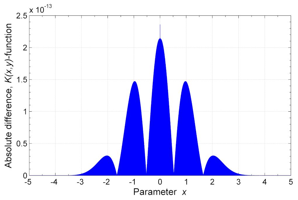
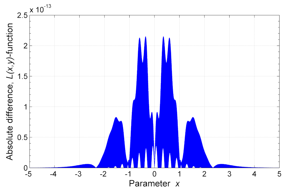
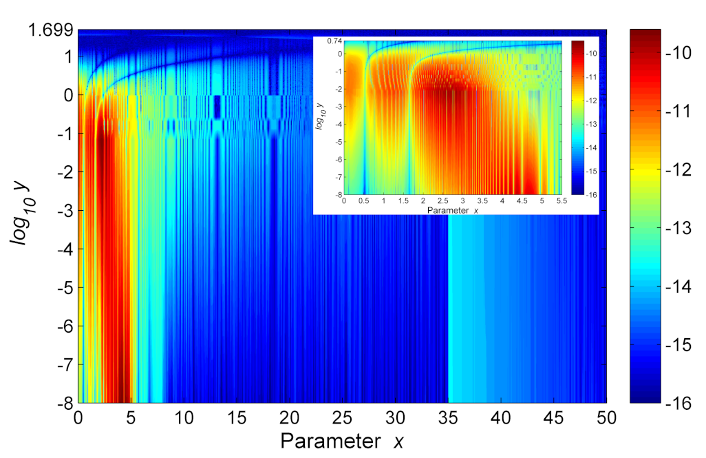
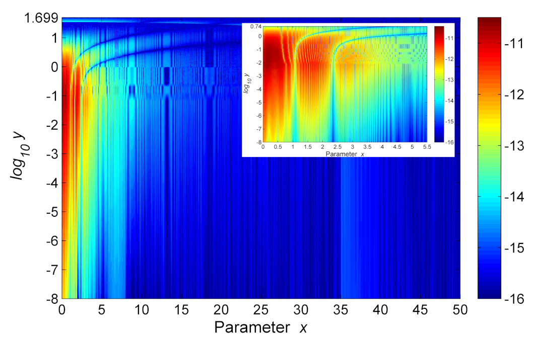
Previously we have reported a new algorithm based on a vectorized interpolation over a single-domain [33]. Such an approach provides accuracy better than ${10}^{-6}$ at $y\ge {10}^{-8}$ for the HITRAN [13] applications. However, this implementation has several limitations. In particular, there is a limitation $\left|x\right|\le {10}^5$. Although it is possible to increase the range for more than ${10}^5$, it requires to introduce more interpolation grid-points for precomputation. Furthermore, this MATLAB implementation accepts an input only as a vector (one dimensional array) or as a scalar.

One of the ways to implement an efficient algorithm is to use an approximation based on the two-domain scheme that we proposed in our earlier publication [23]

$$K\left(x,y\right)\approx \left\{\begin{array}{cccc}& \mathrm{interpolation},\hfill & & \frac{x^2}{{27}^2}+\frac{y^2}{{15}^2}\le 1\hfill \\ & \frac{a_1+b_1{x}^2}{a_2+b_2{x}^2+x^4},\hfill & & \frac{x^2}{{27}^2}+\frac{y^2}{{15}^2}>1,\hfill \end{array}\right.$$

(17a)

where the coefficients are [20]

$$\begin{array}{cc}& a_1=y/\left(2\sqrt{\pi }\right)+y^3/\sqrt{\pi }\approx 0.2820948y+0.5641896y^3\hfill \\ & b_1=y/\sqrt{\pi }\approx 0.5641896y\hfill \\ & a_2=0.25+y^2+y^4\hfill \\ & b_2=-1+2y^2\hfill \end{array}$$

such that

$$\frac{a_1+b_1{x}^2}{a_2+b_2{x}^2+x^4}=Re\left\{\frac{\left(i/\sqrt{\pi }\right)}{z-\frac{1/2}{z}}\right\}.$$

Consequently, the complex error function can also be approximated as [33]

$$w\left(z\right)=K\left(x,y\right)+iL\left(x,y\right)\approx \left\{\begin{array}{cccc}& \mathrm{interpolation},\hfill & & \frac{x^2}{{27}^2}+\frac{y^2}{{15}^2}⩽1\hfill \\ & \frac{\left(i/\sqrt{\pi }\right)}{z-\frac{1/2}{z}},\hfill & & \frac{x^2}{{27}^2}+\frac{y^2}{{15}^2}>1.\hfill \end{array}\right.$$

(17b)

Although the algorithms for the Voigt and complex error functions, built on Equations (17a) and (17b) can provide rapid computations, their accuracies deteriorate at $y<{10}^{-6}$.

In order to resolve this problem we developed a new algorithm that utilizes the internal MATLAB built-up features. Unlike interpolation algorithms shown in [23,33], the proposed approach implies that the number of the interpolation grid-points required for precomputation is not constant and dependent on the input parameter y such that

$$N_{gp}=\frac{1}{\sqrt{y}}+\delta ,$$

(18)

where $\delta$ is the offset that was found experimentally to be $5\times {10}^3$. The corresponding interpolation grid-points range is bounded by $\left[-r,r\right]$, where $r=35$ is the radius that was also found experimentally. The interpolation grid-points are distributed non-equidistantly in logarithmic scale to increase their density near the origin along the x axis.

Equation (18) is entirely empirical. It is reasonable to suggest that the number of the interpolation grid-points should be increased with decreasing y. However, taking the reciprocal of $y^n$, such that $n\ge 1$, results in a very rapid increase of the interpolation grid-points $N_{gp}$ with decreasing y. Our experimental results show that a more or less optimal value $N_{gp}$ can be found by taking the reciprocal of $\sqrt{y}$. The parameter $\delta$ in Equation (18) is to provide a sufficient number of the interpolation grid-points $N_{gp}$ within the internal domain $|x+iy|\le r$ as parameter y increases.

The use of Equation (18) is given as a basic for applications. If higher accuracy is required, the number of the interpolation grid-points $N_{gp}$ can be further increased by using, for example, a modified form of the equation above

$$N_{gp}=\frac{2}{\sqrt{y}}+3\delta .$$

Such a modification improves accuracy by an order of the magnitude.

The algorithm utilizes two domains, internal and external, that are bounded by a circle of radius $\left|x+iy\right|=r$. The internal domain is situated within the circle while the external domain is situated outside of it.

All points within internal domain $\left|x+iy\right|\le r$ are computed by the MATLAB built-in interpolation function interp1 though interpolation grid-points that are computed by using the function file fadsamp.m provided in our article [30]. The spline method was found to be the best for interpolation.

All points outside external domain $\left|x+iy\right|>r$ are computed by the following approximation

$$w\left(z\right)\approx \frac{\left(i/\sqrt{\pi }\right)}{z-\frac{1/2}{z-\frac{1}{z-\frac{3/2}{z}}}}$$

that represents a simplified version of Equation (7) above.

The parameter y is dependent on temperature and pressure. Therefore, it is related to the atmospheric height. In a radiative transfer model, the atmospheric column is sliced into layers [5,6]. The layers can be considered homogeneous if their thicknesses are small enough. Typically, a thickness of 50m (or 20 layers per km) is sufficient to consider the layer homogeneous for atmospheric modeling. This implies that, within a given layer, the temperature and pressure are constants. Since the density of air in the mesosphere is extremely low, its contribution to the radiance is practically negligible. Consequently, taking into consideration that only the troposphere and stratosphere, with an atmospheric column corresponding to a height of up to 40–50km, actually contribute to the radiance, we can conclude that the total number of layers as well as elements for parameter y does not exceed 1000 per gas in atmosphere. However, in many practical tasks, for a single value y at a given atmospheric temperature and pressure, we may need to cover a wide spectral range with high resolution. This signifies that the number of elements for parameter x can exceed a million. Since the number of elements for parameter y is much smaller than the number of elements for parameter x, it is reasonable to implement a configuration in which parameter x is an array and parameter y is a scalar. This approach is more rapid in the MATLAB implementation since the application of a 2D array $M\times N$, where N and M are numbers of elements for parameters x and y, respectively, requires considerably more computer memory.

As it has been mentioned above, the computation of the interpolation grid-points in its original version of the function file w2dom.m is performed by external function fadsamp.m. However, any other MATLAB function file that can provide highly accurate computation of the complex error function may also be used for computation of interpolation grid-points. For example, the function files such as fadf.m [27] and fadfunc.m [31] can also be used as alternatives. The script of the function file w2dom.m is given in Appendix A.

4. Error Analysis

In order to exclude the rounding and truncation errors in computation by using the most recent HITRAN database [13], the values of the $K\left(x,y\right)$ and $L\left(x,y\right)$ functions with 6 or more accurate decimal digits in their mantissas are required. Therefore, in radiative transfer applications involving the HITRAN database, the accuracy of computation of these functions has to be better than ${10}^{-6}$.

Figure 1 shows the absolute difference $\left|K_{ref.}\left(x,y\right)-K\left(x,y\right)\right|$, where $K_{ref.}\left(x,y\right)$ is a highly accurate reference, in the range $-5\le x\le 5$ at $y={10}^{-8}$. As we can see, the absolute difference does not exceed $2.5\times {10}^{-13}$.

Figure 2 shows the absolute difference $\left|L_{ref.}\left(x,y\right)-L\left(x,y\right)\right|$, where $L_{ref.}\left(x,y\right)$ is a highly accurate reference, in the range $-5\le x\le 5$ also at $y={10}^{-8}$. We can see that for the imaginary part the absolute difference also does not exceed $2.5\times {10}^{-13}$.

For more rigorous error analysis, we can apply the following relative errors

$${\mathrm{\Delta }}_{Re}=\frac{\left|K_{ref.}\left(x,y\right)-K\left(x,y\right)\right|}{K_{ref.}\left(x,y\right)}$$

and

$${\mathrm{\Delta }}_{Im}=\frac{\left|L_{ref.}\left(x,y\right)-L\left(x,y\right)\right|}{L_{ref.}\left(x,y\right)}$$

for the real and imaginary parts of the complex error function $w\left(z\right)$, respectively.

Figure 3 depicts the relative error for the real part of the complex error function $Re\left[z\right]=K\left(x,y\right)$ in the domain $0\le x\le 50$ and $0\le y\le {10}^{1.699}$, where ${10}^{1.699}\approx 50$. Inset in Figure 3 shows the smaller domain near the origin $0\le x\le 5.5$ and $0\le y\le {10}^{0.74}$, where ${10}^{0.74}\approx 5.5$. Beyond this smaller domain the observed color is blue indicating that the relative error is below ${10}^{-12}$. As we can see from Figure 3, the relative error does not exceed ∼${10}^{-10}$.

Figure 4 illustrates the relative error for the imaginary part of the complex error function $Im\left[z\right]=L\left(x,y\right)$ in the domain $0\le x\le 50$ and $0\le y\le {10}^{1.699}$. Inset in Figure 4 shows the smaller domain near origin $0\le x\le 5.5$ and $0\le y\le {10}^{0.74}$. Beyond this smaller domain the color is blue and the relative error is below ${10}^{-12}$. As we can see from Figure 4, the relative error is generally lower in the imaginary part and does not exceed ∼${10}^{-11}$.

It is commonly known that the accuracy of $K\left(x,y\right)$ and $L\left(x,y\right)$ functions tend to deteriorate when y decreases [2,16,21,22,28]. However, from Figure 3 and Figure 4 we can see that the decrease of the parameter y does not deteriorate the accuracy. This is possible to achieve since in accordance with Equation (18) the number of the interpolation grid-points $N_{gp}$ increases with decreasing y. Therefore, this technique enables us to resolve efficiently this problem in computation of the complex error function $w\left(z\right)$.

5. Run-Time Test

The run-time test was performed with MATLAB function files wTrap.m [37], fadsamp.m [31] and w2dom.m at equidistantly distributed 10 million points for parameter x at $y={10}^{-8}$. The results of the run-time test are shown in

Table 1. Run-time of algorithms for 10 million points at three different ranges.

Algorithm	Run-Time in Seconds
	$\mathit{x}\in \left[-\mathbf{10},\mathbf{10}\right]$	$\mathit{x}\in \left[-{\mathbf{10}}^{\mathbf{2}},{\mathbf{10}}^{\mathbf{2}}\right]$	$\mathit{x}\in \left[-{\mathbf{10}}^{\mathbf{3}},{\mathbf{10}}^{\mathbf{3}}\right]$
wTrap.m	2.41	2.55	2.45
fadsamp.m	4.14	1.78	1.54
w2dom.m	1.23	1.04	0.98

.

It has been reported that both algorithms wTrap.m and fadsamp.m are highly accurate in computation [37]. In particular, the maximum values in relative errors for the algorithms wTrap.m and fadsamp.m are found to be ∼${10}^{-15}$ and ∼${10}^{-14}$, respectively. However, the computational speed of these two algorithms differs depending on the range for the input parameter x. In particular, Table 1 shows that at smaller range for parameter x the function file wTrap.m performs computation faster than the function file fadsamp.m. However, as the range for parameter x increases, our algorithm fadsamp.m becomes faster. The run-time test also reveals that the algorithm w2dom.m is always faster regardless of the chosen range. This is particularly evident when the range for the input parameter x is smaller.

Table 2. Run-time of algorithms for 30 million points at three different ranges.

Algorithm	Run-Time in Seconds
	$\mathit{x}\in \left[-\mathbf{10},\mathbf{10}\right]$	$\mathit{x}\in \left[-{\mathbf{10}}^{\mathbf{2}},{\mathbf{10}}^{\mathbf{2}}\right]$	$\mathit{x}\in \left[-{\mathbf{10}}^{\mathbf{3}},{\mathbf{10}}^{\mathbf{3}}\right]$
wTrap	8.38	8.33	8.42
fadsamp	14.37	6.02	5.21
w2dom	3.78	3.07	2.86

shows the results of the run-time test at 30 million equidistantly distributed points for parameter x at $y={10}^{-8}$. As we can see, the algorithm w2dom.m remains more rapid proportionally at extended size of the input array as compared to the wTrap.m and fadsamp.m algorithms.

The MATLAB code for the run-time test is provided in Appendix B. The scripts of function files wTrap.m and fadsamp.m can be accessed from the cited literature [30,37], respectively.

6. Conclusions

A new algorithm for the efficient computation of the Voigt/complex error function is shown. We propose a two-domain scheme where the number of interpolation grid-points $N_{gp}$ is dependent on parameter y. The error analysis shows that our MATLAB implementation meets the requirements for radiative transfer applications utilizing the HITRAN molecular spectroscopic database. The run-time test we performed shows that this MATLAB implementation can provide rapid computation especially at smaller ranges of parameter x.

References

1. Faddeyeva, V.N.; Terent’ev, N.M. Tables of the Probability Integral w ( z ) = e z 2 ( 1 + 2 i π 0 z e t 2 d t ) for Complex Argument; Pergamon Press: Oxford, UK, 1961. [Google Scholar]
2. Armstrong, B.H. Spectrum line profiles: The Voigt function. J. Quant. Spectrosc. Radiat. Transf. 1967, 7, 61–88. [Google Scholar] [CrossRef]
3. Gautschi, W. Efficient computation of the complex error function. SIAM J. Numer. Anal. 1970, 7, 187–198. [Google Scholar] [CrossRef]
4. Abramowitz, M.; Stegun, I.A. Error Function and Fresnel Integrals. Handbook of Mathematical Functions with Formulas, Graphs, and Mathematical Tables, 9th ed.; Cambridge University Press: New York, NY, USA, 1972; pp. 297–309. [Google Scholar]
5. Edwards, D.P. Atmospheric transmittance and radiance calculations using line-by-line computer models. Proc. SPIE Model. Atmos. 1988, 928, 94–116. [Google Scholar] [CrossRef]
6. Quine, B.M.; Drummond, J.R. GENSPECT: A line-by-line code with selectable interpolation error tolerance. J. Quantit. Spectrosc. Radiat. Transf. 2002, 74, 147–165. [Google Scholar] [CrossRef]
7. Jagpal, R.K.; Quine, B.M.; Chesser, H.; Abrarov, S.; Lee, R. Calibration and in-orbit performance of the Argus 1000 spectrometer—The Canadian pollution monitor. J. Appl. Remote Sens. 2010, 4, 049501. [Google Scholar] [CrossRef]
8. Berk, A.; Hawes, F. Validation of MODTRAN®6 and its line-by-line algorithm. J. Quant. Spectrosc. Radiat. Transf. 2017, 203, 542–556. [Google Scholar] [CrossRef]
9. Pliutau, D.; Roslyakov, K. Bytran -|- spectral calculations for portable devices using the HITRAN database. Earth Sci. Inform. 2017, 10, 395–404. [Google Scholar] [CrossRef]
10. Siddiqui, R.; Jagpal, R.; Quine, B.M. Short wave upwelling radiative flux (SWupRF) within near infrared (NIR) wavelength bands of O2, H2O, CO2, and CH4 by Argus 1000 along with GENSPECT line by line radiative transfer model. Canad. J. Remote Sens. 2017, 43, 330–344. [Google Scholar] [CrossRef]
11. Siddiqui, R.; Jagpal, R.K.; Abrarov, S.M.; Quine, B.M. Efficient application of the Radiance Enhancement method for detection of the forest fires due to combustion-originated reflectance. J. Environ. Protect. 2021, 12, 717–733. [Google Scholar] [CrossRef]
12. Jagpal, R.K.; Siddiqui, R.; Abrarov, S.M.; Quine, B.M. Effect of the instrument slit function on upwelling radiance from a wavelength dependent surface reflectance. Nature Sci. 2022, 14, 133–147. [Google Scholar] [CrossRef]
13. Hill, C.; Gordon, I.E.; Kochanov, R.V.; Barrett, L.; Wilzewski, J.S.; Rothman, L.S. HITRANonline: An online interface and the flexible representation of spectroscopic data in the HITRAN database. J. Quant. Spectrosc. Radiat. Transf. 2016, 177, 4–14. [Google Scholar] [CrossRef]
14. Balazs, N.L.; Tobias, I. Semiclassical dispersion theory of lasers. Phil. Trans. R. Soc. Lond. A 1969, 264, 1–29. [Google Scholar] [CrossRef]
15. Chan, L.K.P. Equation of atomic resonance for solid-state optics. Appl. Opt. 1986, 25, 1728–1730. [Google Scholar] [CrossRef] [PubMed]
16. Humlíček, J. Optimized computation of the Voigt and complex probability functions. J. Quant. Spectrosc. Radiat. Transf. 1982, 27, 437–444. [Google Scholar] [CrossRef]
17. Drummond, J.R.; Steckner, M. Voigt-function evaluation using a two-dimensional interpolation scheme. J. Quant. Spectrosc. Radiat. Transf. 1985, 34, 517–521. [Google Scholar] [CrossRef]
18. Poppe, G.P.M.; Wijers, C.M.J. More efficient computation of the complex error function. ACM Transact. Math. Software 1990, 16, 38–46. [Google Scholar] [CrossRef]
19. Schreier, F. The Voigt and complex error function: A comparison of computational methods. J. Quant. Spectrosc. Radiat. Transf. 1992, 48, 743–762. [Google Scholar] [CrossRef]
20. Kuntz, M. A new implementation of the Humlicek algorithm for calculation of the Voigt profile function. J. Quant. Spectrosc. Radiat. Transf. 1997, 51, 819–824. [Google Scholar] [CrossRef]
21. Wells, R.J. Rapid approximation to the Voigt/Faddeeva function and its derivatives. J. Quant. Spectrosc. Radiat. Transf. 1999, 62, 29–48. [Google Scholar] [CrossRef]
22. Letchworth, K.L.; Benner, D.C. Rapid and accurate calculation of the Voigt function. J. Quant. Spectrosc. Radiat. Transf. 2007, 107, 173–192. [Google Scholar] [CrossRef]
23. Abrarov, S.M.; Quine, B.M.; Jagpal, R.K. A simple interpolating algorithm for the rapid and accurate calculation of the Voigt function. J. Quant. Spectrosc. Radiat. Transf. 2009, 110, 376–383. [Google Scholar] [CrossRef]
24. Pagnini, G.; Mainardi, F. Evolution equations for the probabilistic generalization of the Voigt profile function. J. Comput. Appl. Math. 2010, 233, 1590–1595. [Google Scholar] [CrossRef]
25. Imai, K.; Suzuki, M.; Takahashi, C. Evaluation of Voigt algorithms for the ISS/JEM/SMILES L2 data processing system. Adv. Space Res. 2010, 45, 669–675. [Google Scholar] [CrossRef]
26. Zaghloul, M.R.; Ali, A.N. Algorithm 916: Computing the Faddeyeva and Voigt Functions. ACM Trans. Math. Software 2011, 38, 15. [Google Scholar] [CrossRef]
27. Abrarov, S.M.; Quine, B.M. Efficient algorithmic implementation of the Voigt/complex error function based on exponential series approximation. Appl. Math. Comput. 2011, 218, 1894–1902. [Google Scholar] [CrossRef]
28. Amamou, H.; Ferhat, B.; Bois, A. Calculation of the Voigt Function in the region of very small values of the parameter a where the calculation is notoriously difficult. Am. J. Anal. Chem. 2013, 4, 725–731. [Google Scholar] [CrossRef]
29. Abrarov, S.M.; Quine, B.M. Sampling by incomplete cosine expansion of the sinc function: Application to the Voigt/complex error function. Appl. Math. Comput. 2015, 258, 425–435. [Google Scholar] [CrossRef]
30. Abrarov, S.M.; Quine, B.M.; Jagpal, R.K. A sampling-based approximation of the complex error function and its implementation without poles. Appl. Num. Math. 2018, 129, 181–191. [Google Scholar] [CrossRef]
31. Abrarov, S.M.; Quine, B.M. A rational approximation of the Dawson’s integral for efficient computation of the complex error function. Appl. Math. Comput. 2018, 321, 526–543. [Google Scholar] [CrossRef]
32. Wang, S.; Huang, S. Evaluation of the numerical algorithms of the plasma dispersion function. J. Quant. Spectrosc. Radiat. Transf. 2019, 234, 64–70. [Google Scholar] [CrossRef]
33. Abrarov, S.M.; Quine, B.M.; Siddiqui, R.; Jagpal, R.K. A single-domain implementation of the Voigt/complex error function by vectorized interpolation. Earth Sci. Res. 2019, 8, 52–63. [Google Scholar] [CrossRef]
34. Kumar, R. The generalized modified Bessel function and its connection with Voigt line profile and Humbert functions. Adv. Appl. Math. 2020, 114, 101986. [Google Scholar] [CrossRef]
35. Nordebo, S. Uniform error bounds for fast calculation of approximate Voigt profiles. J. Quant. Spectrosc, Radiat. Transf. 2021, 270, 107715. [Google Scholar] [CrossRef]
36. Pliutau, D. Combined “Abrarov/Quine-Schreier-Kuntz (AQSK)” algorithm for the calculation of the Voigt function. J. Quant. Spectrosc. Radiat. Transf. 2021, 272, 107797. [Google Scholar] [CrossRef]
37. Al Azah, M.; Chadler-Wilde, S.N. Computation of the complex error function using modified trapezoidal rules. SIAM J. Numer. Anal. 2021, 59, 2346–2367. [Google Scholar] [CrossRef]
38. Copeland, B.J. The Essential Turing: Seminal Writings in Computing, Logic, Philosophy, Artificial Intelligence, and Artificial Life: Plus the Secrets of Enigma; Oxford University Press Inc.: New York, NY, USA, 2004. [Google Scholar]
39. Turing, A.M. A method for the calculation of the zeta-function. Proc. Lond. Math. Soc. 1945, s2-48, 180–197. [Google Scholar] [CrossRef]
40. Trefethen, L.N.; Weideman, J. The exponentially convergent trapezoidal rule. SIAM Rev. 2014, 56, 385–458. [Google Scholar] [CrossRef]
41. Goodwin., E. The evaluation of integrals of the form f ( x ) e x 2 d x . Math. Proc. Cambridge Phil. Soc. 1949, 45, 241–245. [Google Scholar] [CrossRef]
42. Chiarella, C.; Reichel, A. On the evaluation of integrals related to the error function. Math. Comput. 1968, 22, 137–143. [Google Scholar] [CrossRef]
43. Matta, F.; Reichel, A. Uniform computation of the error function and other related functions. Math. Comp. 1971, 25, 339–344. [Google Scholar] [CrossRef]
44. Hunter, D.; Regan, T. A note on the evaluation of the complementary error function. Math. Comp. 1972, 26, 539–541. [Google Scholar] [CrossRef]
Figure 1. Absolute difference for the real part K x , y of the complex error function.
Mathematics 10 03451 g001
Figure 2. Absolute difference for the imaginary part L x , y of the complex error function.
Mathematics 10 03451 g002
Figure 3. Relative error Δ R e for the real part K x , y of the complex error function. Inset shows the relative error Δ R e in the area near the origin.
Mathematics 10 03451 g003
Figure 4. Relative error Δ I m for the imaginary part L x , y of the complex error function. Inset shows the relative error Δ I m in the area near the origin.
Mathematics 10 03451 g004