Article

Generation of Boxes and Permutations Using a Bijective Function and the Lorenz Equations: An Application to Color Image Encryption

by
Víctor Manuel Silva-García
1,
Rolando Flores-Carapia
1,
Manuel Alejandro Cardona-López
2,* and
Miguel Gabriel Villarreal-Cervantes
1
1
Instituto Politécnico Nacional, IPN-CIDETEC, Ciudad de México 07738, Mexico
2
Instituto Politécnico Nacional, Centro de Investigación en Computación, Ciudad de México 07738, Mexico
*
Author to whom correspondence should be addressed.
Mathematics 2023, 11(3), 599; https://doi.org/10.3390/math11030599
Submission received: 12 December 2022 / Revised: 11 January 2023 / Accepted: 20 January 2023 / Published: 24 January 2023
(This article belongs to the Special Issue Numerical Analysis and Scientific Computing II)

Abstract

:
Some images that contain sensitive information and travel through the network require security. Therefore, a symmetric cryptosystem that encrypts images and resists known attacks is developed. Subsequently, in this work, an encryption algorithm known as Image Cipher utilizing Lorenz equation and a Bijective Function—ICLEBF are proposed. In the proposal, the Lorenz equations and the Bijective function are used to generate boxes, the permutation, and schedule keys, considering that all these elements are different in each encryption process. The encryption procedure consists of 14 rounds, where a different box is applied in each round. In this type of algorithm, the impact of quantum computers will be less forceful and can be useful for that epoch. On the other hand, the quality of the encrypted images and the loss of sharpness in decoded images with damage are measured. In addition, an attack from five types of noise (one of which is a developed proposal) is carried out by applying it to encrypted images. Finally, the results of the proposed ICLEBF are compared with other recent image encryption algorithms, including the Advanced Encryption Standard. As a result, this proposal resists known attacks and others that the current standard does not support.

1. Introduction

Large amounts of sensitive information can be sent over the network using images leading to the development of robust encryption systems employed to encrypt them [1,2,3,4,5]. In the same way, Lorenz equations have been widely applied in the different design stages of cryptosystems for image ciphering [6,7,8,9]. In this research, a fourteen-round symmetric algorithm is proposed, that is based on the Lorenz equations and the bijective function. Furthermore, the distribution of keys and signs is based on the elliptic curve [10].
Regarding the security of the ICLEBF cryptosystem, three aspects are studied. First, the security of the proposed symmetric cryptosystem is analyzed according to known attacks such as differential, linear, algebraic, and brute force. For example, the differential attack is evaluated according to the following parameters: Number of Pixels Change Rate (NPCR), Unified Average Changing Intensity (UACI), and Avalanche Criteria (AC) [11]. In addition, it must be taken into account that both the boxes and the permutation involved in the encryption are different in each process; that is, they are variables [12].
Regarding the second aspect, the encrypted images are damaged using five types of noise. The five noises are: additive, multiplicative, Gaussian, occlusion, and a noise that is related to the Chi-Square ( χ 2 ) distribution. A median filter of 5 × 5 is also applied to the damaged decrypted images to complement the process and improve their sharpness. On the other hand, images decoded with noise are evaluated according to a parameter that the authors refer to as the Similarity Parameter (SP). The SP parameter is proposed in this research to evaluate the loss of sharpness in damaged images. The resistance of the proposed algorithm to noise attacks with respect to the AES–CBC [13] cryptosystem is also compared and analyzed.
The third aspect involves an attack on the elliptic curve that is included in the proposal to distribute the keys of the symmetrical system, resulting in the discrete logarithm problem [14]. This point is addressed by comparing the discrete logarithm attack with the factorization of a natural number n having two prime factors, p , q , each of which has approximately the same number of digits [15].
The generation of schedule keys is carried out by randomly choosing a point on the elliptic curve and the Lorenz equations. Furthermore, according to another randomly generated point on the curve, and using a bijective function that goes from the set of non-negative integers to the set of permutations [15], the boxes involved in each round are built; plus, a permutation of the image size. Note that a S -box 8 × 8 is a permutation of 256 elements.
The quality of the encrypted images is measured according to the following elements: entropy, three-way correlation, discrete Fourier transform, energy, homogeneity, contrast, NPCR, UACI, AC, and a goodness-of-fit test using the χ 2 [16]. In some countries, compression with loss of information is not accepted; for instance, in Mexico [17], the images have to accomplish a 512 × 512 pixel size in BMP format. In addition, the ICLEBF cryptosystem was developed for software implementation in Java.
The present work is organized as follows: Section 2 presents the tools that are employed in this research. Section 3 presents the construction of the elements involved in the encryption algorithm and the test images. Section 4 shows the construction of different noises and their application to encrypted images. In addition, a high-level description of the median filter 5 × 5 and the SP parameter is made. The results are shown in Section 5, and their analysis and discussion are presented in Section 6. Finally, Section 7 presents the conclusions and future work.

2. Materials and Methods

A high-level description of the tools required in the proposal is presented in the next section.

2.1. Elliptic Curve

ICLEBF is a symmetric cryptosystem based on two points on the elliptic curve and the use of the Lorenz equations. Therefore, it is convenient to provide a general description of the elements used to generate the elliptic curve. First, the equation of the discrete elliptic curve is written in Equation (1):
y 2 x 3 + a x + b mod p
This work uses a prime number p greater than 2 512 . The prime p is related to the equation p = a 1 2 + a 2 2 considering a 1 as an odd number, a 2 as an even number, p mod 4 ≡ 1, and ( a 1 + a 2 ) mod 4 ≡ 1. Set the constant b = 0 and a = k , the Equation (1) results in Equation (2).
y 2 x 3 k x mod p
On the other hand, the constant k must satisfy that k p 1 / 2 mod p 1 and k p 1 / 4 mod p 1 [18]. In addition, the proposed elliptic curve must meet certain conditions to avoid cryptanalysis attacks known as the MOV attacks or to generate a trace one curve since the latter is considered weak [19]. The conditions are presented in Equations (3) and (4).
# E ( F q ) 1 mod p
# E ( F q ) p
where q = p + 2 a 1 + 1 4 must be a prime number and # E ( F p ) = p + 2 a 1 + 1 represents the total number of solutions of the curve [20]. If q does not result in a prime number, the prime number q must be changed.
On the other hand, the curve’s equation must have three different real roots (non-singular solutions). This requirement is expressed in Equation (5).
4 ( ( k ) 3 ) 0 mod p
It is possible to generate a curve that meets all these requirements by using an algorithm [21]. It is pointed out that in the solution set of the curve, it is possible to define the addition operation (+), which makes this set an abelian group [22].
In the calculation of the sums, the operation of the multiplicative inverse module p is used. This operation is performed using Euclid’s extended algorithm [23]. However, it is possible to perform the calculations differently to reduce execution times. In Section 3, we will prove a theorem and propose an algorithm for calculating the multiplicative inverse.
Since the number of solutions q is prime, then there are some elements in the solution set that generate all the others, i.e., any point P of the solution set can be written as P = k α , where α is the generator element [24]. In fact, a curve is defined if k , p , q , and α are known.
To conclude this section, an example is provided below:
Example. Given a 1 = 341 and a 2 = 40, it follows that p is 117881. It can be verified that p mod 4 ≡ 1, and a 1 + a 2 ≡ 1 mod 4. A primitive element is selected, namely α = (95360, 92352), and k value is given by k = 85264. Then, k is verified using Equations (6) and (7). Therefore the resulting curve is: y 2 x 3 85264 x mod 117881.
85264 117881 1 / 4 mod 117881 1
85264 117881 1 / 2 mod 117881 1
To verify the primitive element α , it must meet that ( q 1 ) [ α = ( x , y ) ] = ( x , y ) . In this case, we have ( 29641 1 ) ( 95360 , 92352 ) = ( 95360 , 92352 ) , taking into account that q = 29641 . The total number of solutions is # E ( F 117881 ) = 118564. In addition, it meets the following conditions: 29641 mod 117881 1, 4 85264 3 mod 117881 0 and # E ( F 29641 ) 117881 . So, the curve is not supersingular, not singular and neither trace one.

2.2. Lorenz Equations

The Lorenz equations describe the atmospheric phenomenon of convection, and they are expressed according to Equations (8)–(10) [7].
x ˙ = τ ( x + y )
y ˙ = r x y x y
z ˙ = b x + x y
The critical points are obtained when Equations (8)–(10) are equal to zero. Furthermore, the values τ , r , and b are considered positive real numbers. From here, it is not difficult to obtain the following critical points: Q 1 = ( 0 , 0 , 0 ) , Q 2 = ( b ( r 1 ) , b ( r 1 ) , r 1 ) y Q 3 = ( b ( r 1 ) , b ( r 1 , r 1 ) .
In this investigation, the values τ = 10 and b = 8 / 3 are chosen. The solution to this system of equations is written as in Equation (11).
X = ξ e λ t
Considering that the Lorenz equations describe the phenomenon of convection in the Earth’s atmosphere, the following parameters are set as: σ = 10 and b = 8 3 . The solution to the Lorenz system of equations has the form X = ξ e λ t where ξ represents the eigenvectors, and λ the eigenvalues.
On the other hand, to calculate the solutions in the neighborhood of the point Q 2 , we start from the equation where the matrices B, X and X are described in Equations (12), (13) and (14), respectively.
B = 10 10 0 r 1 8 / 3 ( r 1 ) 8 / 3 ( r 1 ) 8 / 3 ( r 1 ) 8 / 3
X = x y z
X = x y z
The eigenvalues are calculated from the characteristic polynomial, which is obtained from Equation (15).
B λ I = 0
Considering that the parameter r = 28 , the characteristic polynomial is expressed in Equation (16).
3 λ 3 + 41 λ 2 50 λ + 2160 = 0
From Equation (16), one real root and two complex ones are obtained; these are written in Equations (17)–(19).
λ 1 = 22.558424
λ 2 = 4.445878 + 3.485904 i
λ 3 = 4.445878 3.485904 i
Regarding the eigenvectors, it is only necessary to generate two of them to obtain the general solution. Equations (20) and (21) show the eigenvectors ξ 1 and ξ 2 , where c = 4.445878.
ξ 1 = 9.163288 11.507650 1
ξ 2 = 0.359510 + 0.116796 i 0.478680 + 0.294040 i 1 + 0 i
u ( t ) = 0.3595 cos ( 3.4859 ) t 0.1167 sin ( 3.4859 ) t 0.4786 cos ( 3.4859 ) t 0.2940 sin ( 3.4859 ) t cos ( 3.4859 ) t e c
v ( t ) = 0.1167 cos ( 3.4859 ) t 0.3595 sin ( 3.4859 ) t 0.2940 cos ( 3.4859 ) t 0.4786 sin ( 3.4859 ) t sin ( 3.4859 ) t e c
Note that the solution ξ 2 e ( 4.445878 + 3.485904 i ) t contains a real part and a complex part. The real part is presented as u and the complex one as v × i , where u and v are expressed in Equations (22) and (23). Furthermore, if we set w = ξ 1 e 22.5584 t , the general solution is then written in Equation (24).
X ( t ) = e 22.5584 t D 1 ξ 1 + D 2 u ( t ) + D 3 v ( t ) × i
In this work, the second coordinate of vectors that appear in Equation (24) is taken, resulting in ϕ y ( t ) . Considering that the constant D 1 of the general solution becomes equal to zero, and the variable t takes the value t 1 = 1 / 4.445878 , ϕ y ( t 1 ) results in Equation (25).
ϕ y ( t 1 ) = ( 0.4750 ) D 2 e + ( 0.2881 ) D 3 e
In practice, although a finite sequence of decimals is taken, this does not imply that the conditions of Chaos are not met.

2.3. Correlation Coefficient

The correlation coefficient, or simply correlation, is calculated in three directions. The correlation parameter is a measure of the figure quality; furthermore, it is used in many works of this kind of research [25,26].
The procedure to carry out this measurement is explained next: m pixels are randomly selected from the encrypted image. Subsequently, for each one of them, the pixels adjacent to it are taken, that is, in the horizontal, vertical, and diagonal directions. For example, suppose we want to analyze the vertical direction for the color green. So, each of these m pixels has the green color, which ranges from the values 0 to 255, denoting this value as x g . Next, the adjacent pixel in the vertical direction is taken. This pixel has the green color with a certain level that varies in the same way as the previous one. Therefore, let us call it y g .
Hence, the formulas to calculate the correlation in the vertical direction for the green color are presented in the Equation (26). The terms x ¯ g , y ¯ g are the averages of x g and y g , and their calculations are shown in Equations (27) and (28).
r v ; x g , y g = 1 m ( i = 1 m ( x i , g x ¯ g ) ( y i , g y ¯ g ) ) ( 1 m i = 1 m ( x i , g x ¯ g ) 2 ( 1 m i = 1 m ( y i , g y ¯ g ) 2 ) )
x ¯ g = 1 m i = 1 m x i , g
y ¯ g = 1 m i = 1 m y i , g
The calculation of the correlation in the other directions and colors is very similar.

2.4. Entropy

Another parameter useful to evaluate the encrypted images is the information entropy [27]. This parameter is measured according to Equation (29) [28]. In addition, it is pointed out that this measurement is carried out for each primary color in the case of encrypted images.
In this same order of ideas, it is mentioned that each primary color in an encrypted image is described by 256 levels, represented by a byte. The primary colors are: red, green and blue. From here, an image is well encrypted if the entropy of each color is close to 8. It is pertinent to clarify that this condition is necessary but not sufficient because the distribution of information can have entropy 8, and the information cannot have a random distribution [18].
H ( x ) = x ε X P ( x ) l o g 2 P ( x )
On the other hand, it is pointed out that entropy is not the only parameter used to evaluate encrypted images. In practice, an entropy value close to 8 is associated with a good randomness [29].

2.5. Discrete Fourier Transform

This test is part of the NIST 800-22 [30] standard. It evaluates that there are no repeating patterns in a binary string, which means that it is random. Furthermore, it can be stated that it is a statistical hypothesis test, where the null hypothesis is that the binary string is random, against the alternative one that it is not.
On the other hand, the variables that intervene in this procedure are expressed below.
N 0 is a quantity obtained according to Equation (30), where m represents the chain length of zeros and ones.
The function f j is defined in the Equation (31) where i is the complex number 1 , and the variable x k is equal to ± 1 .
Once the function f j is defined, the variable N 1 is determined as the number of times that f j is less than the value h; considering that it is defined as: h = Ln 1 0.05 ( m ) .
Taking into account the variables N 0 , N 1 ; the variable d is represented in Equation (32).
On the other hand, the function e r f c d 2 is represented in Equation (33). Based on the above, the decision rule P v a l u e = e r f c d 2 is defined as follows:
If P V a l u e > 0.01, the null hypothesis is accepted; that is, the string of zeros and ones is random; otherwise, it is rejected.
N 0 = ( 0.95 ) × m / 2
f j = k = 1 m x k e 2 π ( i ) ( k 1 ) j n
d = N 1 N 0 n ( 0.95 ) ( 0.05 ) 4
erfc d 2 = 2 ( 1 Φ ( d ) )

2.6. Goodness-of-Fit Test

This tool is a statistical hypothesis test, where the null and alternative hypotheses are as follows:
(I) Null hypothesis. The string of bits is random.
(II) Alternative hypothesis. The string of bits is not random.
In addition, it is necessary to define a statistic and a level of significance, which in this investigation is α = 0.01 [31], that determines a region of acceptance or rejection and, subsequently, the decision rule.
The statistic is shown in Equation (34), which has a χ 2 distribution with n 1 degrees of freedom. Regarding the variables involved in Equation (34), it is noted that o i , e x p correspond to the observed and expected values. Furthermore, considering that each primary color is described with 256 levels (a byte), we conclude that the degrees of freedom are n 1 = 255 . With this argument, and in accordance with the central limit theorem, in this paper we assume that the variable χ 2 approximates a normal distribution N ( μ , σ ) ; where μ = 255 and σ = 22.58 [32].
χ 2 = i = 1 k ( o i exp ) 2 exp
On the other hand, according to the significance level value defined above, it follows that when χ 2 < 308 , the null hypothesis is accepted. On the contrary, it is rejected if χ 2 308 .
Furthermore, it is mentioned that the measurement of the encrypted image quality is carried out for each primary color; red, green, and blue. In addition, it is pointed out that this type of test is not found in the NIST 800-22.

2.7. Parameters NPCR, UACI and AC

In this research, three parameters are used to measure the strength of ICLEBF to differential attacks and the quality of encryption. These parameters are: NPCR, UACI, and AC.
Equation (35) describes the NPCR parameter, where the subscript c indicates the primary color; red, green, or blue. Regarding the elements that intervene in it, it is mentioned that the function D ( i , j ) proceeds as follows: it is equal to 1 when the bytes in position ( i , j ) of the encrypted images have the same value. On the contrary, it presents a zero value when they are different. It is important to point out that the flat images are only different by one byte. The variables W , H represent the width and height of the image. The value considered appropriate for this parameter is a percentage close to 99.6 % [33].
NPCR c = Σ i , j D ( i , j ) c W × H × 100 %
Equation (36) describes the value of UACI, considering that the variable C ( i , j ) l , c is in a range from 0 to 255 and corresponds to the l-th encrypted images. As commented before, the flat images are only different by one byte. On the other hand, ( i , j ) and c correspond to the byte position and the primary color.
The value considered adequate for this parameter is 33.4 % [34].
UACI c = 1 W × H [ Σ i , j C 1 , c C 2 , c 255 ] × 100 %
Equation (37) describes the parameter AC, where the function b ( i , j ) is equal to 1 when the pixels of images related to the position ( i , j ) are the same. Otherwise, b ( i , j ) is equal to 0. The variable T represents the number of bits in the image. Likewise, to resist the differential attack, it is considered that AC is close to 50 % [35]. In addition, the subscript c indicates the type of primary color that is analyzed.
AC c = Σ i , j b ( i , j ) c T × 100 %

2.8. Parameters of Homogeneity, Contrast, Energy and Median Filter

In many image encryption investigations, Contrast, Homogeneity, and Energy parameters are used to assess the quality of encryption. Each of them is briefly described below.
Regarding Homogeneity, it is evaluated with Equation (38), considering that ( i , j ) are the coordinates of the pixel and g ( i , j ) its value at that position. On the other hand, an image is said to be “well” encrypted when the Homogeneity values are small, i.e., the smaller the Homogeneity value, the higher the quality of the encryption obtained [36].
H o m o g e n e i t y = i , j g ( i , j ) 1 + i j
Equation (39) represents the Contrast parameter, which measures the degree of inequality between a pixel and its neighbors. We then say that the encryption of an image is “good” if the contrast values are large. In the results section, the obtained values are compared with other investigations [37]. The function g ( i , j ) provides the value of g in the pixel ( i , j ) .
C o n t r a s t = i , j i j 2 g ( i , j )
The third parameter, Energy, is evaluated according to Equation (40). This parameter measures the degree of disorder between the pixels. The closer this value is to zero, the greater the disorder, which implies that the encryption is “good” [38].
E n e r g y = i , j g ( i , j ) 2

2.9. Median Filter

It is clear that when damage is inflicted upon the encrypted image, there will be a loss of sharpness in the decrypted image. Therefore, improving the sharpness of the decrypted image with damage is convenient and thus complements this process. This represents the motivation in this work to use a median filter 5 × 5 [39]. In this sense, a filter manipulates neighboring pixels of size ( n × m ) in a general perspective.
Hence, the median filter 5 × 5 proceeds as follows: given any pixel ( x 1 , x 2 ) of the image map, a mask of 25 pixels is constructed, leaving the point ( x 1 , x 2 ) in the center, and the other pixels as its neighbors. Table 1 illustrates this aspect.
From here, it is possible to order these 25 values according to their intensity, and then the value that meets the following requirement is chosen as the median: it is greater than or equal to the first 25 2 1 element, i.e., the 50 % , and less than the remaining points.
Because in this investigation the analysis is carried out for each of the primary colors (red, green and blue), the median of each of these colors are then denoted as follows: M r , ( x 1 , x 2 ) , M g , ( x 1 , x 2 ) and M b , ( x 1 , x 2 ) , respectively.
Finally, the intensity value of each of the mask points is replaced by the median value.

3. Model Development

In this section, the theorem to compute the multiplicative inverse of a number when the modulus is prime, the encryption algorithm, and the generations of permutations and boxes using an algorithm that defines a bijective function [21] are described.

3.1. Calculation of the Multiplicative Inverse

The multiplicative inverse modulo p is used by following the next theorem:
Theorem 1.
Given a prime number p, and an element x ϵ Z p such that x 0 , then the multiplicative inverse modulo p of x is calculated as: x p 2 mod p.
Proof of Theorem 1.
Since p is prime, the greatest common divisor (gcd) gcd ( x , p ) = 1. So, it is stated that x has an inverse, and it is also unique.
From here,
x p 2 × x = x p 1 mod p
However, x p 1 mod p ≡ 1. According to Lagrange theorem [40] and considering that Euler’s ϕ satisfies ϕ ( p ) = p 1 , then, x p 2 is the multiplicative inverse of x. □
The advantage of computing the multiplicative inverse modulo p according to Theorem 1 is that this process is parallelizable [40], in contrast to Euclid’s algorithm, whose procedure for calculating the inverse is sequential.

3.2. SP Parameter

The SP parameter is proposed to evaluate the loss of sharpness in the decrypted images with damage. This parameter is represented by Equation (41), where the subscript c indicates the primary color type.
SP c = | 100 UACI c ( 2.994 ) |
In this work, the UACI instrument defined in Equation (36) is used to produce SP, taking into account the following argument.
Because UACI evaluates the differences C 1 , c C 2 , c between two images, which in this case would be the original and the decrypted with damage, it can be seen that when the two images are the same, UACI = 0, and therefore, SP = 100; however, if UACI ≊ 33 % , which happens when the image is well encrypted, it follows that SP ≊ 0. The factor 2.994 indicates the range of SP from 0 to 100.
So, the parameter SP provides information about the degree of similarity between two images.

3.3. Algorithm for the Generation of Permutations

Given a positive integer n, the following set is defined: Z n = m N 0 m n ! 1 . Any element of Z m can be expressed according to Equation (42). That is, express it on a factorial basis.
m = A 0 ( n 1 ) ! + A 1 ( n 2 ) ! + A n 2 ( 1 ) ! + A n 1 ( 0 ) !
On the other hand, according to the division algorithm, the A i are unique. Moreover, that A n 1 = 0 . Thus, the values A i satisfy Equation (43).
0 A i < ( n i ) with 0 i ( n 2 )
Recent research uses the above arguments to develop an algorithm that builds permutations in a set of n different elements [21]. In this paper, this set is { 0 , 1 , n 1 } .
Furthermore, it is shown that the algorithm defines a bijective function [41]. The latter is highlighted because it is convenient that there are two different permutations for two positive integers m 1 , m 2 Z n . The above allows for building dynamic permutations and boxes for a cryptosystem.

3.4. Cipher Procedure

The high-level description of the ICLEBF cryptosystem consists of a 14-round symmetric encryption algorithm [42]. In this algorithm, both the permutations, the 8 × 8  S-box, and the schedule keys are dynamic, i.e., in each encryption procedure, they are different. Furthermore, the size of permutations and the schedule keys are the same as the image size. Below, we present the steps of the algorithm in each round.
(I) The encryption algorithm applies a permutation P , on the pixel positions of the original image. This is done before the rounds start. Next, the xor operation is performed between the string that results from the permutation and the first schedule key. Subsequently, the string that results from the xor operation is divided into 8-bit substrings, i.e., a byte. Finally, the substitution operation is applied to each of these bytes, using the first 8 × 8  S-box. The criteria used in the substitution operation are the same as in FIPS 197 [43]. Later, the permutation P , boxes, and schedule keys are generated.
(II) From rounds two to thirteen, the algorithm executes the following steps: it starts with an xor between the output of the previous round and the corresponding schedule key. Then, the substitution operation is performed with the corresponding 8 × 8  S-box.
(III) In round 14, the following steps are executed: first, the xor operation is applied between schedule key 14 and the output of round 13. Next, the result of the previous operation is subdivided into blocks of 8 bits, and the substitution process is then carried out with the last box. It is terminated with an xor operation with schedule key 15. This last result provides the encrypted image.
Regarding the construction of the permutation, the schedule keys and the boxes are shown in the next section.

3.5. Generation of the S-Boxes, Permutation, and Schedule Keys

The procedure for generating the 8 × 8 S-boxes is shown below:
(a) An integer C 1 is randomly obtained that satisfies 0 < C 1 < 2 512 . Subsequently, the point C 1 α is calculated, where α is the primitive number. Let us denote the result C 1 α = ( w 1 , w 2 ) .
(b) In this investigation, the constant D 3 of Equation (25) is proposed. It has a value associated with the binary string w 1 w 2 . Afterward, the operations 0.2881 D 3 e are performed.
(c) According to the result of section (b), the bits from the decimal point to the right are divided into blocks of 8 bits. Furthermore, it is clarified that an 8 × 8  S-box is a permutation of the 256 elements of the set { 00 , 01 , f f } . The constants A i of Equation (42) are computed, and then the permutation is obtained. In this order of ideas, the calculation of A 0 is done as follows: the first 8 bits after the decimal point are taken, and the integer associated with this string of bits is called a 0 . Then, the following calculation is carried out: A 0 = a 0 mod 256, such that 0 A 0 < 256 holds. A i is related to the i-th block of 8 bits to the right of the decimal point. This block has an associated integer value which we denote as a i . So, A i = a i mod 256 - i with 0 i < 255 , considering that A 255 = 0.
(d) Once the A i has been obtained, the algorithm outlined in Section 3.3 is used to generate the permutation. To get the other boxes, i.e., from two to fourteen, continue to shift to the right of the 8-bit decimal point and then perform the modular operation.
Regarding the generation of the permutation, the procedure is shown below.
(a) In the same way as before, an integer C 2 is randomly generated, that is in a range of 0 < C 2 < 2 512 .
(b) Once the value C 2 is obtained, the point C 2 α is calculated, considering that α is the primitive number. Let us write the result of C 2 α as ( z 1 , z 2 ) . Then, the concatenation of the coordinates of ( z 1 , z 2 ) is performed; that is, z 1 z 2 . The integer value associated with the binary string z 1 z 2 is assigned to the constant D 2 of the Equation (25).
(c) According to the previous step, the calculation ( 0.4750 × e ) D 2 is carried out. So, in this investigation, it is proposed to divide the binary string formed from the decimal point to the right into blocks of three bytes; that is, it starts with bytes 0, 1, 2. Let us refer to the non-negative integer associated with the binary string of the first three bytes as b 0 ; furthermore, let us denote the number of pixels in the image as l. With this information, the first constant, A 0 , of Equation (42) is calculated as follows: A 0 = b 0 mod l 0 . To obtain the constant A i with i > 0 , we will proceed as follows: i shifts one byte to the right of the decimal point, and the bytes i , i + 1 , i + 2 are taken. In the same way as before, this 24-bit block has a non-negative integer, which is written as b i . From here, the i-th constant is obtained as follows: A i = b i mod l i .
(d) When the constants indicated in Equation (42) are calculated, it is possible to generate a permutation as mentioned in Section 3.3.
On the other side, the previous steps are essentially described below. A positive integer C 1 is chosen, that satisfies the condition where it is less than the number of solutions ( 2 512 ) . This value leads us to a point on the curve ( w 1 , w 2 ) . The previous point generates the integer D 3 = w 1 w 2 . From here, it is possible to execute the operation indicated in Equation (25). Blocks of one byte are taken to the right of the decimal point. Each byte can be interpreted as an integer and used to obtain the A i constants in Equation (42). Subsequently, a permutation is obtained over an array of 256 positions, which leads us to a box.
Regarding the schedule keys (third aspect), the same calculations in items (a) and (b) are performed to obtain the permutation of bytes of the image. Then, the constant C 2 is used.
Subsequently, the decimal point to the right l pixels are obtained from the product ( 0.4750 × e ) D 2 ; that is, a binary string of the image size. This paper sets this string as the first schedule key, denoted as k 1 . To generate the other schedule keys; that is, k 2 k 15 the following is done:
For k i with i > 1 , a one-byte left circular shift of the key k i 1 is performed.
In order to illustrate the point, the elliptic curve used in this investigation is shown below. Furthermore, it is pointed out that the proposed curve meets the conditions mentioned in Equations (3)–(5).
The values of p , q , a , b , k , as well as, the primitive element α = ( x 1 , x 2 ) are expressed next.
  • p = 988464ba59685284506433ccd3f83450166fda2d2ec7
    109a5c0679434e9dfb46b3a447043b406c4115af9a2c7fdc17
    bc9b6668f07d80d7142f534a1dc64ef400b9b2100acb691
  • q = 2621192e965a14a114190cf334fe0d14059bf68b4bb1
    c42697019e50d3a77ed1ace911d9c1e6fa9ecb772f44670d2
    9e05a69fc249b108ed06114d9e01b7662721ecf151ce2329
  • a = 31662dbf1d0c1691728e2c47e26720c3d0f760b216aa8
    00eb153c54ae3e0c522345eb09
  • b = 308
  • k = 870eebe8cf19ece84593dd9deaec2ebab1380c94c240fe
    8fc1d45836fff18114c42308e5aafef0ee4d1a643b179415eb
    34d8b2118e51ad727b63efc5dba104179bcece5a0d7cb
On the other hand, the generator element α = ( x 1 , x 2 ) is presented below:
  • x 1 = 28b1f61561824dac022aa29d37df70295a2d7f34f696
    5e032d85b35b6e4c8403a47922b96753ba338061a05eee5
    30f5759043d58aa09d69ae8b2377b640c01e484ac14d27d
    693
  • x 2 = 288189d9988f9d839ae797195f3a4b512b36773156af
    fd0b64a5ed740c9ea059233eab4765397a0a5de87ea46a20
    d208cf8988d433e4d703792e2f950ad6a0a631f0d424e6951
In another order of ideas, it can be seen that the points ( w 1 , w 2 ) and ( z 1 , z 2 ) are important in constructing the symmetric cryptosystem. So, in a secure communication scheme, for example, the PKI [44], the recipient only needs to know these points to develop the particular symmetric cryptosystem. In this sense, the sender can send the points mentioned above using the recipient’s public key called Q. Later, the recipient using their private key can get ( w 1 , w 2 ) and ( z 1 , z 2 ) . Furthermore, the sender can sign the message according to the Elliptic Curve Signature Algorithm (ECSA) [45] standard.

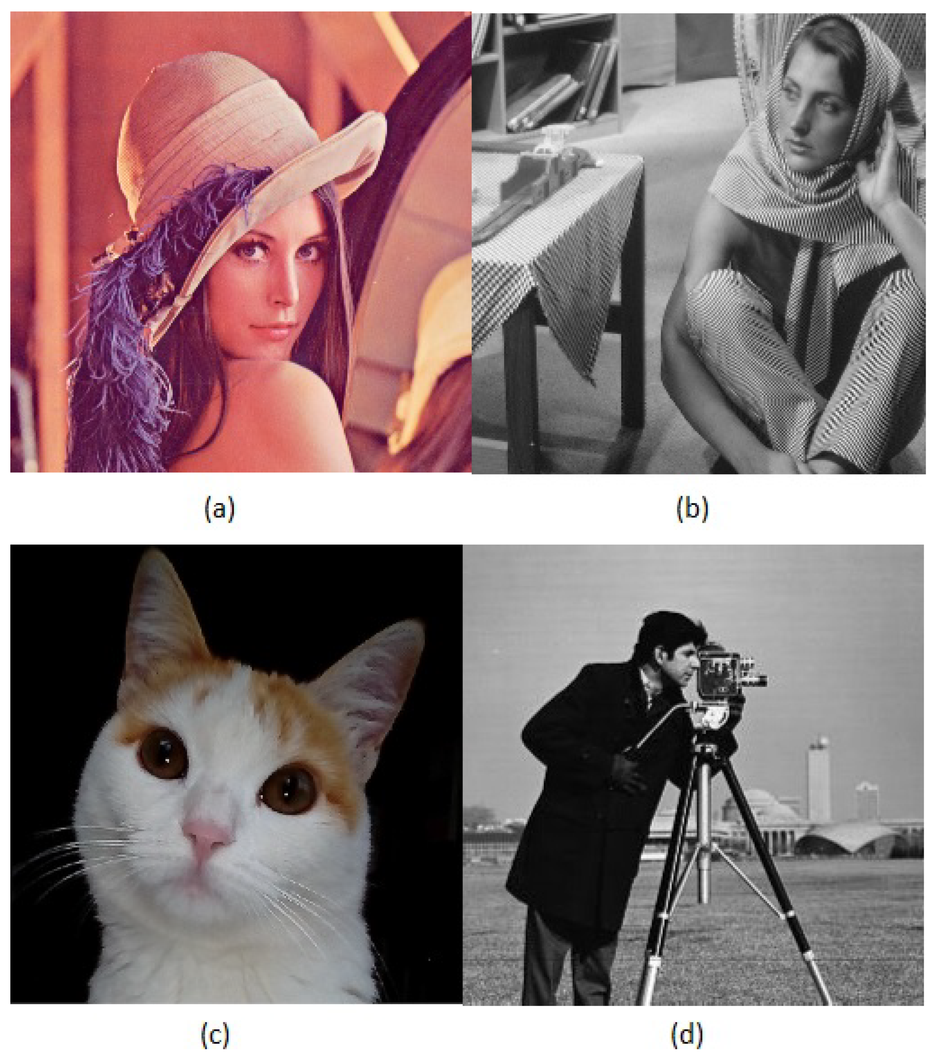
3.6. Images Used to Evaluate ICLEBF

Figure 1 shows the images used in this research to evaluate the encryption quality of the proposed cryptosystem. The size of the images is 512 × 512 pixels, according to the convention used in this kind of research work [46], although they can be of different dimensions.
The Barbara and Cameraman images (Figure 1b and Figure 1d, respectively) are used to test the proposed encryption algorithm because, when using 256-gray-level images, there is a risk of poor-quality encryption if a secret-key cryptosystem is used. In fact, this is why AES is not used as a standard in image encryption, and the AES–CBC [47] cryptosystem is instead employed. Furthermore, in those images, parts are entirely white, and in the other image, parts are completely black.
On the other hand, Figure 1a is widely known in the encryption field; the Lena image. Furthermore, in this research, the image of Vicky in Figure 1c is used, and both images are in color, i.e., the three primary colors appear, red, green, and blue, with 256 levels for each one.
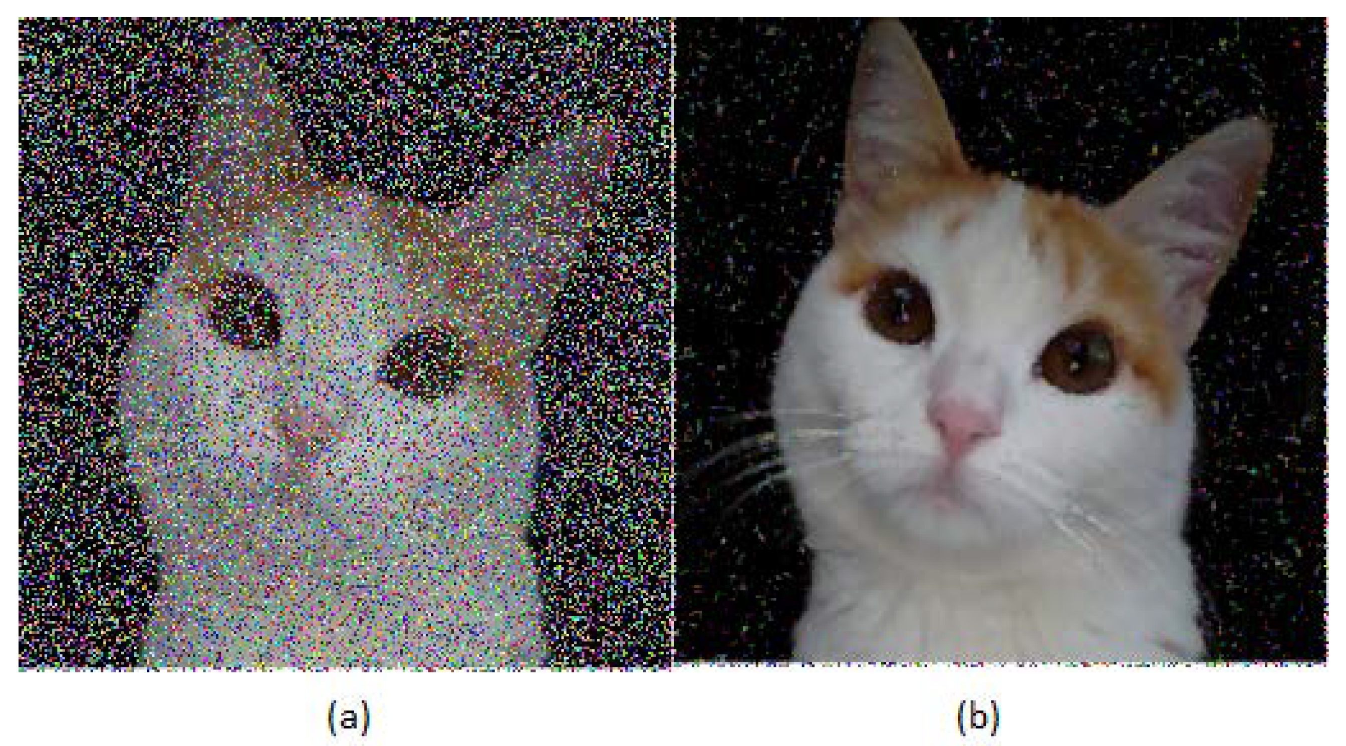
To conclude this section, it is noted that Figure 1c is encrypted with AES–CBC, and then an occlusion noise damage of 40% of the encrypted figure size is applied. This is later decrypted. The previous result is compared with that obtained when the same procedure is carried out, except that Figure 1c is now encrypted with the ICLEBF algorithm. Finally, in the “Result” section, the comparison is shown.

4. Damage in Encrypted Images

This work employs five types of noise and applies them to images encrypted with ICLEBF. These noises are the following: χ 2 , Gaussian, occlusion, additive and multiplicative; considering that in this research, the noise χ 2 is proposed. On the other hand, the parameter Similarity Parameter (SP) defined above is proposed to evaluate the damage in sharpness. In addition, a median filter 5 × 5 is applied to complement the process.

4.1. Noise Generated by the Variable χ 2

This section begins with a description of the noise χ 2 , that is based on the random variable χ 2 = i = 1 k ( o i exp ) 2 exp . Considering that the noise χ 2 is presented in Section 2 and using the central limit theorem, this noise variable is distributed as a normal variable, with a mean μ = 255 and a standard deviation σ = 22.58 .
Furthermore, the images damaged in this research have two domains: spatial and frequency. The process begins with the choice of n points at random in the spatial domain of the encrypted image. These points have an associated intensity in the frequency domain, which we call I c ; furthermore, it satisfies 0 I c 255 . The subscript indicates the primary color type.
Once the n points, denoted as ( x , y ) , have been chosen for each color, a value z c N(0, 1) is randomly chosen. Subsequently, we calculate the value I c according to Equation (44).
I c ( x , y ) = 255 + z c ( x , y ) 42.5
The next step is to assign an integer value to the variable I c , i.e., this variable is discretized. In this sense, we will use the symbols ⌊⌋ and ⌈⌉ as follows: when the decimal part of I c is less than or equal to 0.5, the integer part is taken I c , which is denoted as I c . Otherwise, when the decimal fraction is greater than 0.5, the integer part plus one of I c is taken. The above is denoted as I c .
In this work, the discretized value of I c is denoted as I d c and is calculated according to Equation (45).
I d c ( x , y ) = 255 + z c ( x , y ) 42.5 mod 256
It is necessary to replace the value of I c with I d c to apply the noise to the encrypted image. Furthermore, note that the symbols ⌊⌋ or ⌈⌉ in Equation (45) are used as appropriate. Before concluding this section, it is important to mention that the vast majority of the intensities (95%) are replaced by values that fall within the following ranges: [0, 84] or [170, 255]; i.e., by extreme values.

4.2. Additive and Multiplicative Noises

In the same way, as in the previous section, there are two domains. In this sense, n points ( x , y ) are randomly chosen from the spatial domain, that is, from the encrypted image; each has an associated intensity I c that complies with 0 I c 255 .
In the case of additive noise, for each point ( x , y ) and color, an integer γ ( x , y ) is chosen at random, and then the calculations indicated in Equation (46) are done. To apply the additive noise, proceed as follows: the value of I c is replaced by I c , obtained in Equation (46).
I c ( x , y ) = [ I c ( x 1 , x 2 ) + γ ( x 1 , x 2 ) ] mod 256
The procedure of the multiplicative noise is similar to the additive one. In fact, the value of I c is obtained according to Equation (47). Then, to apply the multiplicative noise shown in Equation (47), the value of I c is replaced by I c .
I c ( x , y ) = [ I c ( x 1 , x 2 ) × γ ( x 1 , x 2 ) ] mod 256

4.3. Gaussian Noise

This part analyzes the application of Gaussian noise, which leads to the random variable x with a standard normal distribution, i.e., x N(0, 1).
In this sense, in the spatial domain, n points ( x 1 , x 2 ) are randomly chosen according to the uniform distribution. These points also have an associated intensity I c , which meets the following condition: 0 I c 255 .
In this work, the intensity I c is calculated according to Equation (48) considering that z N(0, 1). Furthermore, it is mentioned that the values of z are obtained with a standard normal distribution generator; that is, z N(0, 1). In addition, the following rule applies: when the value of z generated with this standard normal distribution is less than −3, this takes the value z = 3 . On the contrary, when the generated value is greater than 3, this takes the value z = 3 . It follows that the range of z is [−3, 3].
I c = 127.5 + z × ( 42.5 )
The symbols , and , are used to discretize the variable I c . In this sense, it proceeds as follows: when the decimal fraction of I c is less than or equal to 0.5, only the integer part is considered, and the above is denoted as I d c = I c . On the other hand, if the decimal fraction is greater than 0.5, then the integer part plus one is taken, and this is denoted as I d c = I c .
From here, it is proposed to apply the Gaussian noise to the encrypted image in the following way: the value of I c is replaced by that of I d c = I c or I d c = I c according to the case. On the other hand, 95% of the substituted values are in the interval [42, 212]; i.e., centered around 127.5.

4.4. Occlusion Noise

The occlusion noise is applied in the following way: the intensity of all points of a concentric parallelogram is replaced by a single color, which in this investigation is a cherry color.
As can be seen, the above is equivalent to producing noise inside the concentric parallelogram. In order to clarify ideas, this procedure is illustrated in Figure 2.

5. Results

First, we will show the results of encrypted images without damage and later the results when damaged. In addition, it starts with the correlation and entropy parameters. Subsequently, the NPCR, UACI, AC, energy, contrast, and homogeneity measurements are presented. Later, the parameters that apply hypothesis tests are described.
Figure 3 shows how the ICLEBF algorithm encrypts. In this sense, it is mentioned that regardless of whether the flat image (original) is in color or 256 levels of gray, the encrypted figure will always be in color. The encrypted image is Figure 1b (Barbara).

5.1. Correlation and Entropy

Table 2 presents the results of the correlation when the test images of Figure 1 are encrypted.
Table 3 shows the entropy results. As pointed out previously, only results are presented in this part. Later, the corresponding analysis will be made.
Table 4 shows a comparative results of Lena entropy with other cryptosystems.

5.2. Results of NPCR, UACI, AC, Energy, Contrast and Homogeneity

Table 5, Table 6 and Table 7 present the results of NPCR, UACI and AC, respectively. On the other hand, the energy, contrast and homogeneity are presented in Table 8, Table 9 and Table 10.

5.3. Discrete Fourier Transform and Goodness-of-Fit Test

This part shows the parameters’ results, including a statistical hypothesis test. Table 11 presents the measurements obtained when the parameter of the discrete Fourier transform is applied to the encrypted images of Figure 1, and Table 12 illustrates the values obtained when using the goodness-of-fit test in the encrypted figures of the four test images.

5.4. Tests on Black or White Images

The purpose of conducting tests on entirely black or white images is because ICLEBF defines a symmetric cryptosystem. Subsequently, the encryption may not perform correctly. For this reason, the measurements of NPCR, UACI, and AC are carried out in the encrypted figures, one of the images in black and the other in white. In this sense, the results are reported in Table 13. Furthermore, the size of both images is set to 512 × 512 pixels.

5.5. Result of Encrypted Images with Noise

We start this section by showing Figure 4, which has three images. The first, Figure 4a presents Barbara’s flat (original) image. In the second one, Figure 4b, Barbara’s image is encrypted with the AES–CBC algorithm, and then multiplicative noise is applied to the encrypted figure at 40% of its size. Finally, in the last Figure 4c, Barbara is encrypted with the ICLEBF algorithm, then multiplicative noise is applied to 40% of the encrypted figure and it is subsequently decrypted.
On the other hand, Figure 5 illustrates the case of the Vicky image shown in Figure 1c, which is encrypted with AES–CBC (Figure 5a), and then occlusion noise is applied to 40% of the encrypted image (Figure 5b). In this sense, Figure 6 shows the case in which the Vicky image is encrypted with the ICLEBF algorithm, and then the occlusion noise is applied to 40% of the encrypted figure, as shown in Figure 6a. It is later deciphered, resulting in Figure 6b.
Regarding the application of the median filter of 5 × 5 to complement the procedure, the deciphered images with noise are evaluated using the SP parameter to know the degree of improvement in sharpness. It is observed in Figure 7b the improvement of the sharpness of Vicky’s image when the median filter 5 × 5 is applied to the damaged image. It is also important to comment that the Vicky image is encrypted with the ICLEBF algorithm. Furthermore, in Table 14 the sharpness evaluation is shown based on the SP parameter results. Different damage sizes χ 2 are applied to the encrypted test images in this case. On the other hand, Table 15 shows the SP parameter results when five types of noise are applied from 40% of the size of the encrypted test images, and the filter 5 × 5 is used to improve sharpness.

6. Discussion

Considering that the security of the ICLEBF algorithm is essential, we begin with possible attacks on the proposed cryptosystem. Later, an attack on the elliptic curve is observed, and then those that damage the encrypted figures.
In this order of ideas, the proposed cryptosystem attacks include the following: differential, linear, brute force, and algebraic. Regarding the differential attack, Table 5, Table 6 and Table 7 show the results of the encrypted figures of the test images. It is observed that their values are in the desired range, i.e., NPCR around 99.6%, UACI values close to 33.3%, and AC around 50%. Therefore, it can be concluded that it resists differential attack. Regarding the linear attack, it is mentioned that the boxes are unknown since they are different in each encryption process, which means that the linear attack cannot be carried out as described in [51]. In addition, due to this same characteristic, the algebraic attack cannot be carried out either. Regarding the brute force attack, the following consideration is made: taking into account that when two points of the curve are known, the proposed cryptosystem can be built; furthermore, considering that the number of solutions is q > 2 512 , it follows that the complexity of the problem is greater than ( 2 512 ) 2 . This is larger than the complexity of AES-256, and has not yet been solved by brute force [52].
The elliptic curve attack leads to the discrete logarithm problem, which consists of discovering the private key m when the public key Q is known. On the other hand, the discrete logarithm problem on the curve is equivalent to factoring a positive integer n in the RSA scheme [21]. In this sense, when the number of solutions q is a prime larger than 2 512 (which is our case), the discrete logarithm problem is equivalent to factoring an n larger than 2 15000 . The above is much larger than the application currently used in the RSA cryptosystem ( 2 4096 [53]).
Two aspects are mentioned regarding the attack on encrypted images using noise: the first refers to a comparison of the proposed algorithm ICLEBF with the algorithm of the AES–CBC standard. Figure 5 and Figure 6 show that ICLEBF better resists the occlusion attack because, after decrypting the damaged image, the original image is still visible. However, this is not the case with AES–CBC. Furthermore, the same happens in Figure 4. Figure 4b illustrates the case when Barbara’s image is encrypted with AES–CBC, then corrupted with multiplicative noise, and deciphered. On the other hand, if the image is encrypted with ICLEBF and the same process is done as before, then Figure 4c is obtained.
The second aspect refers to the application of the median filter 5 × 5 to a decrypted image with corruption. In this sense, Figure 7b illustrates how a damaged image changes when the filter is applied. On the other hand, the IP parameter is applied to damaged images. Table 14 presents the results concerning the extent to which the sharpness deteriorates when χ 2 noise is applied, at different sizes, to the encrypted images of Figure 1. Table 15 shows the extent to which the sharpness improves when the median filter 5 × 5 is applied to the damaged images. It is worth noting that the noise χ 2 of size 40% applied to the Vicky image provides a result of IP 53 % . However, after applying the filter, as shown in Table 15, the IP parameter value is around 93%.
According to the results presented in Table 2, Table 3, Table 4, Table 5, Table 6, Table 7, Table 8, Table 9, Table 10, Table 11 and Table 12, it is affirmed that the image encryption is of sound quality because the color distribution in the encrypted images presents a random behavior. In this sense, the obtained quality is superior to those reported in some recent investigations [2,11,27] and are similar to [1,3,5]. Furthermore, according to the results in Table 13 related to the NPCR, UACI, and AC parameters of the encrypted black and white images, it is observed that they present suitable values [54]. On the other hand, in Table 14, the damages in the encrypted images are evaluated when the noise χ 2 of different sizes are applied to them. This measurement is carried out with the SP parameter. Table 15 evaluates the application of the 5 × 5 filter to images with different types of noise. In this sense, it is highlighted that the Vicky image with noise improves by more than 40 % when the median filter is applied, according to the SP parameter.
Additionally, the algorithm was programmed in Java language, achieving an execution time for encryption/decryption of 0.3 s. This time was registered on a computer with an i9-10900K CPU with 10 cores and Windows 11 operating system.

7. Conclusions

This research proposes a symmetric cryptosystem, ICLEBF, to encrypt color images. The proposed cryptosystem is secure based on two aspects. The first aspect details that the boxes and permutations are dynamic; they are different in each encryption process. The second relates to the number of solutions q of the curve, which in this work is approximately 2 562 . Futhermore, it bears certain advantages over existing cryptosystems, particularly over AES–CBC. Another essential issue to highlight regarding the ICLEBF cryptosystem is that in its construction, an asymmetric cryptosystem was utilized, the elliptic curve, making it possible to distribute its keys. Finally, the main reason behind proposing the current symmetric cryptosystem for the encryption of color images is that this type of cryptosystem will have less impact on quantum computers [18]. This is advantageous because, in this case, only the curve is required and not two cryptosystems, as in the PKI scheme. In addition, it is possible to sign the information. Furthermore, the encryption quality produces outstanding results according to 10 evaluation instruments. Finally, future quantum computers will have a drastic impact on current asymmetric algorithms [18], and thus future work will involve the sending of a seed via a post-quantum cryptosystem [18].

Author Contributions

Conceptualization, methodology, formal analysis, investigation, visualization, V.M.S.-G., R.F.-C. and M.A.C.-L.; writing—review and editing, data curation, software, validation, writing—original draft preparation, V.M.S.-G., R.F.-C., M.A.C.-L. and M.G.V.-C.; resources, supervision, project administration, funding acquisition, V.M.S.-G. All authors have read and agreed to the published version of the manuscript.

Funding

This work was funded in part by the economic support program of the Comisión de Operación y Fomento de Actividades Académicas (COFAA) and the Secretaría de Investigación y Posgrado (SIP) of the Instituto Politécnico Nacional under grant 20220154.

Institutional Review Board Statement

Not applicable.

Informed Consent Statement

Not applicable.

Data Availability Statement

The data that support the findings of this study are available from the corresponding author upon request.

Acknowledgments

The authors would like to thank the Instituto Politécnico Nacional of México (Secretaría Académica, Comisión de Operación y Fomento de Actividades Académicas COFAA, SIP, and CIDETEC), and the CONACyT (SNI) for their support in the development of this work.

Conflicts of Interest

The authors declare no conflict of interest.

Abbreviations

The following abbreviations are used in this manuscript:
ICLEBFImage Cipher utilizing Lorenz Equation and a Bijective Function
NPCRNumber of Pixels Change Rate
UACIUnified Average Changing Intensity
ACAvalanche Criteria
SPSimilarity Parameter
SPNSubstitution Permutation Network
RSARivest–Shamir–Adleman

References

  1. Alexan, W.; ElBeltagy, M.; Aboshousha, A. RGB Image Encryption through Cellular Automata, S-Box and the Lorenz System. Symmetry 2022, 14, 443. [Google Scholar] [CrossRef]
  2. Sani, R.H.; Behnia, S.; Akhshani, A. Creation of S-box based on a hierarchy of Julia sets: Image encryption approach. Multidimens. Syst. Signal. Process. 2022, 33, 39–62. [Google Scholar] [CrossRef]
  3. Hayat, U.; Ullah, I.; Azam, N.A.; Azhar, S. A Novel Image Encryption Scheme Based on Elliptic Curves over Finite Rings. Entropy 2022, 24, 571. [Google Scholar] [CrossRef]
  4. Murtaza, G.; Azam, N.A.; Hayat, U. Designing an Efficient and Highly Dynamic Substitution-Box Generator for Block Ciphers Based on Finite Elliptic Curves. Secur. Commun. Netw. 2021, 2021, 3367521. [Google Scholar] [CrossRef]
  5. Zhou, S.; Zhao, Z.; Wang, X. Novel chaotic colour image cryptosystem with deep learning. Chaos Solitons Fractals 2022, 161, 112380. [Google Scholar] [CrossRef]
  6. Li, T.; Yan, W.; Chi, Z. A new image encryption algorithm based on optimized Lorenz chaotic system. Concurr. Comput. 2022, 34, e5902. [Google Scholar] [CrossRef]
  7. Ren, H.; Niu, S.; Chen, J.; Li, M.; Yue, Z. A Visually Secure Image Encryption Based on the Fractional Lorenz System and Compressive Sensing. Fractal Fract. 2022, 6, 302. [Google Scholar] [CrossRef]
  8. Rashmi, P.; Supriya, M.C.; Hua, Q. Enhanced Lorenz-Chaotic Encryption Method for Partial Medical Image Encryption and Data Hiding in Big Data Healthcare. Secur. Commun. Netw. 2022, 2022, 9363377. [Google Scholar] [CrossRef]
  9. Tang, M.; Zeng, G.; Yang, Y.; Chen, J. A hyperchaotic image encryption scheme based on the triple dislocation of the Liu and Lorenz system. Optik 2022, 261, 169133. [Google Scholar] [CrossRef]
  10. Bhat, J.; Saqib, M.; Moon, A.H. Fuzzy extractor and chaos enhanced elliptic curve cryptography for image encryption and authentication. Int. J. Syst. Assur. Eng. Manag. 2022, 13, 697–712. [Google Scholar] [CrossRef]
  11. Elsaid, S.A.; Alotaibi, E.R.; Alsaleh, S. A robust hybrid cryptosystem based on DNA and Hyperchaotic for images encryption. Multimed. Tools Appl. 2022, 82, 1995–2019. [Google Scholar] [CrossRef]
  12. Li, M.; Wang, M.; Fan, H.; An, K.; Liu, G. A novel plaintext-related chaotic image encryption scheme with no additional plaintext information. Chaos Solitons Fractals 2022, 158, 111989. [Google Scholar] [CrossRef]
  13. Ametepe, A.F.X.; Ahouandjinou, A.S.; Ezin, E.C. Robust encryption method based on AES-CBC using elliptic curves Diffie–Hellman to secure data in wireless sensor networks. Wirel. Netw. 2022, 28, 991–1001. [Google Scholar] [CrossRef]
  14. Banik, A.; Laiphrakpam, D.S.; Agrawal, A.; Patgiri, R. Secret image encryption based on chaotic system and elliptic curve cryptography. Digit. Signal Process 2022, 129, 103639. [Google Scholar] [CrossRef]
  15. Silva-García, V.M.; Flores-Carapia, R.; Rentería-Márquez, C.; Luna-Benoso, B.; Chimal-Eguía, J.C. Image cipher applications using the elliptical curve and chaos. Int. J. Appl. Math. Comput. Sci. 2020, 30, 377–391. [Google Scholar] [CrossRef]
  16. Shen, C.; Panda, S.; Vogelstein, J.T. The Chi-Square Test of Distance Correlation. J. Comput. Graph. Stat. 2022, 31, 254–262. [Google Scholar] [CrossRef]
  17. General de la Nación, A. Manual de digitalización de documentos. Bol. Arch. General Nación 2022, 9, 41–117. [Google Scholar]
  18. Stinson, D.R.; Patterson, M. Cryptography: Theory and Practice, 4th ed.; CRC Press: Boca Raton, FL, USA, 2018; pp. 278–295. [Google Scholar]
  19. Underwood, R.G. Cryptography for Secure Encryption, 1st ed.; Springer: Cham, Switzerland, 2022; pp. 271–296. [Google Scholar]
  20. Zheng, Z. Modern Cryptography, 1st ed.; Springer: Singapore, 2022; Volume 1, pp. 229–251. [Google Scholar]
  21. Silva-García, V.M.; Flores-Carapia, R.; González-Ramírez, M.D.; Vega-Alvarado, E.; Villarreal-Cervantes, M.G. Cryptosystem Based on the Elliptic Curve With a High Degree of Resistance to Damage on the Encrypted Images. IEEE Access 2020, 8, 218777–218792. [Google Scholar] [CrossRef]
  22. Ali, F.; Rather, B.A.; Fatima, N.; Sarfraz, M.; Ullah, A.; Alharbi, K.A.M.; Dad, R. On the Topological Indices of Commuting Graphs for Finite Non-Abelian Groups. Symmetry 2022, 14, 1266. [Google Scholar] [CrossRef]
  23. Aldaya, A.C.; Sarmiento, A.J.C.; Sánchez-Solano, S. SPA vulnerabilities of the binary extended Euclidean algorithm. J. Cryptogr. Eng. 2017, 7, 273–285. [Google Scholar] [CrossRef]
  24. Cohen, S.D.; Kapetanakis, G.; Reis, L. The existence of Fq-primitive points on curves using freeness. Comptes Rendus Math. 2022, 360, 641–652. [Google Scholar] [CrossRef]
  25. Yu, J.; Li, C.; Song, X.; Guo, S.; Wang, E. Parallel Mixed Image Encryption and Extraction Algorithm Based on Compressed Sensing. Entropy 2021, 23, 278. [Google Scholar] [CrossRef] [PubMed]
  26. Zeng, J.; Wang, C.; Ye, G. A Novel Hyperchaotic Image Encryption System Based on Particle Swarm Optimization Algorithm and Cellular Automata. Secur. Commun. Netw. 2021, 2021, 6675565. [Google Scholar] [CrossRef]
  27. Chai, X.; Fu, J.; Gan, Z.; Lu, Y.; Zhang, Y. An image encryption scheme based on multi-objective optimization and block compressed sensing. Nonlinear Dyn. 2022, 108, 2671–2704. [Google Scholar] [CrossRef]
  28. Shannon, C.E. A mathematical theory of communication. Bell Syst. Tech. J. 1948, 27, 379–423. [Google Scholar] [CrossRef] [Green Version]
  29. Panchikkil, S.; Manikandan, V.; Zhang, Y.D. An efficient spatial transformation-based entropy retained reversible data hiding scheme in encrypted images. Optik 2022, 261, 169211. [Google Scholar] [CrossRef]
  30. Kowalska, K.A.; Fogliano, D.; Coello, J.G. On the Revision of NIST 800-22 Test Suites; Cryptology ePrint Archive, Paper 2022/540; Crypta Labs: London, UK, 2022; Available online: https://eprint.iacr.org/2022/540 (accessed on 11 December 2022).
  31. Liu, Z.; Shen, J.; Barfield, R.; Schwartz, J.; Baccarelli, A.A.; Lin, X. Large-Scale Hypothesis Testing for Causal Mediation Effects with Applications in Genome-wide Epigenetic Studies. J. Am. Stat. Assoc. 2022, 117, 67–81. [Google Scholar] [CrossRef]
  32. Bourgade, P.; Mody, K.; Pain, M. Optimal Local Law and Central Limit Theorem for β-Ensembles. Commun. Math. Phys. 2022, 390, 1017–1079. [Google Scholar] [CrossRef]
  33. Pandurangi Ramacharya, B.; Patil, M.R.; Keralkar, S. Fast partial image encryption with fuzzy logic and chaotic mapping. Evol. Intel. 2022, 1, 1–17. [Google Scholar] [CrossRef]
  34. Arab, A.A.; Rostami, M.J.B.; Ghavami, B. An image encryption algorithm using the combination of chaotic maps. Optik 2022, 261, 169122. [Google Scholar] [CrossRef]
  35. Poojary, A.; Kiran Kumar, V.; Nagesh, H. FPGA implementation novel lightweight MBRISI cipher. J. Ambient. Intell. Humaniz. Comput. 2022, 1, 1–13. [Google Scholar] [CrossRef]
  36. Kiran, P.; Parameshachari, B. Resource Optimized Selective Image Encryption of Medical Images Using Multiple Chaotic Systems. Microprocess. Microsyst. 2022, 91, 104546. [Google Scholar] [CrossRef]
  37. Iqbal, N.; Hanif, M.; Rehman, Z.U.; Zohaib, M. On the novel image encryption based on chaotic system and DNA computing. Multimed. Tools Appl. 2022, 81, 8107–8137. [Google Scholar] [CrossRef]
  38. Asif, M.; Asamoah, J.K.K.; Hazzazi, M.M.; Alharbi, A.R.; Ashraf, M.U.; Alghamdi, A.M. A Novel Image Encryption Technique Based on Cyclic Codes over Galois Field. Comput. Intell. Neurosci. 2022, 2022, 1–9. [Google Scholar] [CrossRef]
  39. Guo, S.; Wang, G.; Han, L.; Song, X.; Yang, W. COVID-19 CT image denoising algorithm based on adaptive threshold and optimized weighted median filter. Biomed. Signal Process. Control 2022, 75, 103552. [Google Scholar] [CrossRef] [PubMed]
  40. Fink, E.; Clarke, P.; Spoerk, M.; Khinast, J. Unsupervised real-time evaluation of optical coherence tomography (OCT) images of solid oral dosage forms. J. Real-Time Image Process. 2022, 19, 881–892. [Google Scholar] [CrossRef]
  41. Gallian, J.A. Contemporary Abstract Algebra, 10th ed.; CRC Press: Boca Raton, FL, USA, 2021; pp. 19–21. [Google Scholar]
  42. Lone, M.A.; Qureshi, S. RGB image encryption based on symmetric keys using Arnold transform, 3D chaotic map and affine hill cipher. Optik 2022, 260, 168880. [Google Scholar] [CrossRef]
  43. Shetty, N.P.; Muniyal, B.; Kaithi, R.R.; Yemma, S.C.R. Comparison of Encryption Techniques to Encrypt Private Parts of an Image. In Proceedings of the Advances in Electrical and Computer Technologies; Sengodan, T., Murugappan, M., Misra, S., Eds.; Springer Nature: Singapore, 2022; pp. 535–557. [Google Scholar] [CrossRef]
  44. Chanda, S.; Luhach, A.K.; Alnumay, W.; Sengupta, I.; Sinha Roy, D. A lightweight device-level Public Key Infrastructure with DRAM based Physical Unclonable Function (PUF) for secure cyber physical systems. Comput. Commun. 2022, 190, 87–98. [Google Scholar] [CrossRef]
  45. Yuvaraj, N.; Praghash, K.; Karthikeyan, T. Data Privacy Preservation and Trade-off Balance Between Privacy and Utility Using Deep Adaptive Clustering and Elliptic Curve Digital Signature Algorithm. Wirel. Pers. Commun. 2022, 124, 655–670. [Google Scholar] [CrossRef]
  46. Chai, X.; Wu, H.; Gan, Z.; Han, D.; Zhang, Y.; Chen, Y. An efficient approach for encrypting double color images into a visually meaningful cipher image using 2D compressive sensing. Inf. Sci. 2021, 556, 305–340. [Google Scholar] [CrossRef]
  47. Zhang, Y.; Chen, A.; Chen, B. A unified improvement of the AES algorithm. Multimed. Tools Appl. 2022, 81, 18875–18895. [Google Scholar] [CrossRef]
  48. Feixiang, Z.; Mingzhe, L.; Kun, W.; Hong, Z. Color image encryption via Hénon-zigzag map and chaotic restricted Boltzmann machine over Blockchain. Opt. Laser Technol. 2021, 135, 106610. [Google Scholar] [CrossRef]
  49. Xingyuan, W.; Junjian, Z.; Guanghui, C. An image encryption algorithm based on ZigZag transform and LL compound chaotic system. Opt. Laser Technol. 2019, 119, 105581. [Google Scholar] [CrossRef]
  50. Yaghouti Niyat, A.; Moattar, M.H.; Niazi Torshiz, M. Color image encryption based on hybrid hyper-chaotic system and cellular automata. Opt. Lasers Eng. 2017, 90, 225–237. [Google Scholar] [CrossRef]
  51. Liu, X.; Tong, X.; Wang, Z.; Zhang, M. Uniform non-degeneracy discrete chaotic system and its application in image encryption. Nonlinear Dyn. 2022, 108, 653–682. [Google Scholar] [CrossRef]
  52. Lin, C.H.; Hu, G.H.; Chan, C.Y.; Yan, J.J. Chaos-Based Synchronized Dynamic Keys and Their Application to Image Encryption with an Improved AES Algorithm. Appl. Sci. 2021, 11, 1329. [Google Scholar] [CrossRef]
  53. Yarom, Y.; Genkin, D.; Heninger, N. CacheBleed: A timing attack on OpenSSL constant-time RSA. J. Cryptogr. Eng. 2017, 7, 99–112. [Google Scholar] [CrossRef]
  54. K.U., S.; Mohamed, A. A novel image encryption scheme using both pixel level and bit level permutation with chaotic map. Appl. Soft Comput. 2020, 90, 106162. [Google Scholar] [CrossRef]
Figure 1. Images used for evaluating ICLEBF: (a) Lena, (b) Barbara, (c) Vicky, (d) Cameraman.
Mathematics 11 00599 g001
Figure 2. Occlusion noise in an encrypted image.
Mathematics 11 00599 g002
Figure 3. Barbara image (a) original and (b) ciphered with AICPBD.
Mathematics 11 00599 g003
Figure 4. Flat image of Barbara (a). Decrypted image of Barbara when a multiplicative noise of size 40% is applied to a figure encrypted with AES–CBC (b). Decrypted image of Barbara when a multiplicative noise of size 40% is applied to a figure encrypted with ICLEBF (c).
Mathematics 11 00599 g004
Figure 5. Image (a) is the Vicky cat image ciphered of Figure 1c using AES–CBC with 40% occlusion damage and (b) is the deciphered image.
Mathematics 11 00599 g005
Figure 6. Vicky cat image (a) ciphered using ICLEBF with 40% occlusion damage and (b) is the deciphered image.
Mathematics 11 00599 g006
Figure 7. (a) The Vicky cat image deciphered with 40% occlusion noise, and (b) deciphered with noise and then median filter is applied.
Mathematics 11 00599 g007
Table 1. A mask of 5 × 5 for the median filter.
( x 1 2 , x 2 + 2 ) ( x 1 1 , x 2 + 2 ) ( x 1 , x 2 + 2 ) ( x 1 + 1 , x 2 + 2 ) ( x 1 + 2 , x 2 + 2 )
( x 1 2 , x 2 + 1 ) ( x 1 1 , x 2 + 1 ) ( x 1 , x 2 + 1 ) ( x 1 + 1 , x 2 + 1 ) ( x 1 + 2 , x 2 + 1 )
( x 1 2 , x 2 ) ( x 1 1 , x 2 ) ( x 1 , x 2 ) ( x 1 + 1 , x 2 ) ( x 1 + 2 , x 2 )
( x 1 2 , x 2 1 ) ( x 1 1 , x 2 1 ) ( x 1 , x 2 1 ) ( x 1 + 1 , x 2 1 ) ( x 1 + 2 , x 2 1 )
( x 1 2 , x 2 2 ) ( x 1 1 , x 2 2 ) ( x 1 , x 2 2 ) ( x 1 + 1 , x 2 2 ) ( x 1 + 2 , x 2 2 )
Table 2. Correlation of the encrypted test images of Figure 1.
ColorCorrelationLenaBarbaraVickyCameraman
Horizontal 0.0004 0.0080 0.0011 0.0061
RedVertical 0.0097 0.0086 0.0034 0.0009
Diagonal 0.0069 0.0034 0.0079 0.0133
Horizontal 0.0037 0.0196 0.0170 0.0014
GreenVertical 0.0052 0.0060 0.0006 0.0131
Diagonal 0.0058 0.0065 0.0174 0.0062
Horizontal 0.0044 0.0198 0.0037 0.0030
BlueVertical 0.0116 0.0021 0.0019 0.0012
Diagonal 0.0009 0.0020 0.0042 0.0146
Table 3. Entropy of the encrypted test images of Figure 1.
ColorLenaBarbaraVickyCameraman
Red 7.99919 7.99935 7.99919 7.99932
Green 7.99929 7.99925 7.99928 7.99926
Blue 7.99923 7.99935 7.99927 7.99947
Table 4. Entropy analysis of Lena Figure 1a.
ColorICLEBF System[48][49][50]
Red 7.9992 7.9921 7.9987 7.9972
Green 7.9993 7.9917 7.9991 7.9973
Blue 7.9992 7.9972 7.9983 7.9972
Table 5. NPCR of the test images after encryption.
ColorLenaBarbaraVickyCameraman
Red 99.609 99.606 99.602 99.603
Green 99.614 99.608 99.598 99.620
Blue 99.613 99.604 99.608 99.620
Table 6. UACI of the test images after encryption.
ColorLenaBarbaraVickyCameraman
Red 33.414 33.437 33.478 33.486
Green 33.461 33.562 33.483 33.452
Blue 33.365 33.468 33.421 33.457
Table 7. AC of the test images after encryption.
ColorLenaBarbaraVickyCameraman
Red 49.997 49.994 50.003 49.996
Green 49.996 50.020 49.985 49.961
Blue 49.963 49.981 50.014 49.944
Table 8. Energy of Figure 1 images after encryption.
ColorLenaBarbaraVickyCameraman
Red 0.0156 0.0156 0.0156 0.0156
Green 0.0156 0.0156 0.0156 0.0155
Blue 0.0156 0.0156 0.0155 0.0156
Table 9. Contrast of Figure 1 images after encryption.
ColorLenaBarbaraVickyCameraman
Red 10.501 10.516 10.475 10.472
Green 10.504 10.450 10.514 10.538
Blue 10.526 10.494 10.503 10.503
Table 10. Homogeneity of Figure 1 images after encryption.
ColorLenaBarbaraVickyCameraman
Red 0.388 0.389 0.390 0.389
Green 0.389 0.389 0.389 0.388
Blue 0.389 0.388 0.389 0.389
Table 11. The randomness measurement using the Discrete Fourier Transform (✓ Accept, x Reject), with α = 0.01 .
ColorLenaBarbaraVickyCameraman
Red 0.671 / 0.978 / 0.342 / 0.093 /
Green 0.368 / 0.116 / 0.737 / 0.272 /
Blue 0.191 / 0.214 / 0.182 / 0.469 /
Table 12. Results of the Goodness-of-Fit test (✓ Accept, x Reject), with α = 0.01 .
ColorLenaBarbaraVickyCameraman
Red 242.9 / 256.3 / 259.3 / 243.9 /
Green 252.7 / 229.8 / 254.6 / 251.9 /
Blue 287.5 / 260.7 / 264.2 / 272.3 /
Table 13. NPCR, UACI and AC values for the completely black and completely white images.
ParameterColorBlack ImageWhite Image
Red 99.610 99.588
NPCRGreen 99.606 99.605
Blue 99.603 99.627
Red 33.429 33.384
UACIGreen 33.428 33.520
Blue 33.480 33.410
Red 50.039 50.005
ACGreen 49.950 49.989
Blue 49.986 50.006
Table 14. SP parameter for distinct noise size of the testing images after encryption, utilizing chi square damage.
ColorSize NoiseLenaBarbaraVickyCameraman
20% 80.17 82.12 77.06 81.44
Red 30 % 70.39 73.25 65.49 72.15
40% 60.26 64.31 54.10 62.75
20% 81.66 82.17 76.83 81.45
Green30% 72.49 73.21 64.86 72.08
40% 63.35 64.28 53.30 62.64
20% 83.43 82.12 76.47 81.34
Blue30% 75.14 73.15 64.68 72.12
40% 66.92 64.33 52.89 62.80
Table 15. SP after a 5 × 5 median filter was applied to encrypted images with 40% damage from different noise sources.
ColorNoise TypeLenaBarbaraVickyCameraman
Chi square 92.39 85.76 93.78 92.38
Additive 92.36 85.81 93.76 92.49
RedMultiplicative 92.54 85.93 94.11 92.57
Gaussian 92.43 85.80 93.81 92.41
Occlusion 92.59 85.84 93.86 92.47
Chi square 90.71 85.85 93.61 92.47
Additive 90.72 85.78 93.59 92.51
GreenMultiplicative 90.87 85.93 93.91 92.52
Gaussian 90.76 85.80 93.75 92.40
Occlusion 90.80 85.87 93.69 92.44
Chi square 91.94 85.85 93.42 92.48
Additive 91.96 85.75 93.53 92.45
BlueMultiplicative 92.03 85.94 93.94 92.60
Gaussian 91.93 85.82 93.63 92.40
Occlusion 91.97 85.87 93.57 92.45
Disclaimer/Publisher’s Note: The statements, opinions and data contained in all publications are solely those of the individual author(s) and contributor(s) and not of MDPI and/or the editor(s). MDPI and/or the editor(s) disclaim responsibility for any injury to people or property resulting from any ideas, methods, instructions or products referred to in the content.

