Article

Mathematical Modeling of the State of the Battery of Cargo Electric Vehicles

by
Nikita V. Martyushev
1,*,
Boris V. Malozyomov
2,
Svetlana N. Sorokova
3,
Egor A. Efremenkov
3 and
Mengxu Qi
3
1
Department of Advanced Technologies, Tomsk Polytechnic University, 634050 Tomsk, Russia
2
Department of Electrotechnical Complexes, Novosibirsk State Technical University, 20, Karla Marksa Ave., 630073 Novosibirsk, Russia
3
Department of Mechanical Engineering, Tomsk Polytechnic University, 30, Lenin Ave., 634050 Tomsk, Russia
*
Author to whom correspondence should be addressed.
Mathematics 2023, 11(3), 536; https://doi.org/10.3390/math11030536
Submission received: 28 December 2022 / Revised: 15 January 2023 / Accepted: 17 January 2023 / Published: 19 January 2023

Abstract

:
In this paper, a mathematical simulation model of an electric vehicle traction battery has been developed, in which the battery was studied during the dynamic modes of its charge and discharge for heavy electric vehicles in various driving conditions—the conditions of the urban cycle and movement outside the city. The state of a lithium-ion battery is modeled based on operational factors, including changes in battery temperature. The simulation results will be useful for the implementation of real-time systems that take into account the processes of changing the characteristics of traction batteries. The developed mathematical model can be used in battery management systems to monitor the state of charge and battery degradation using the assessment of the state of charge (SOC) and the state of health (SOH). This is especially important when designing and operating a smart battery management system (BMS) in virtually any application of lithium-ion batteries, providing information on how long the device will run before it needs to be charged (SOC value) and when the battery should be replaced due to loss of battery capacity (SOH value). Based on the battery equivalent circuit and the system of equations, a simulation model was created to calculate the electrical and thermal characteristics. The equivalent circuit includes active and reactive elements, each of which imitates the physicochemical parameter of the battery under study or the structural element of the electrochemical battery. The input signals of the mathematical model are the current and ambient temperatures obtained during the tests of the electric vehicle, and the output signals are voltage, electrolyte temperature and degree of charge. The resulting equations make it possible to assign values of internal resistance to a certain temperature value and a certain value of the degree of charge. As a result of simulation modeling, the dependence of battery heating at various ambient temperatures was determined.

1. Introduction

In recent years, electric energy storage systems have been considered a key element in the technological development of vehicles and renewable energy. Currently, lithium-ion batteries are the de facto standard in the field of power supplies for electric vehicles, uninterruptible power systems, mobile devices and gadgets [1]. Another example of the use of lithium-ion batteries is storage for renewable energy sources (mainly solar panels and wind turbines). For example, in 2011, China installed a storage device based on lithium-ion batteries with a total capacity of 36 MWh, capable of supplying 6 MW of electrical power to the grid for 6 h [2]. An example from the opposite end of the scale is lithium-ion batteries for implantable pacemakers, the load current of which is on the order of 10 μA [3]. The capacity of a single commercially produced lithium-ion cell has long crossed the mark of 500 Ah [4].
The use of lithium-ion batteries requires compliance with the parameters of the discharge and charge of the battery; otherwise, irreversible degradation of capacity, failure and even fire due to self-heating may occur. Therefore, lithium-ion batteries are always used together with a monitoring and control system—SKU or BMS (battery management system) [5]. The battery management system performs protective functions by monitoring temperature, charge/discharge current and voltage, thus preventing over-discharging, overcharging and overheating. The BMS also monitors the state of the battery by evaluating the degree of charge (state of charge, SOC) and the state of fitness (state of health, SOH). An intelligent battery management system (BMS) is essential in virtually any application of lithium-ion batteries.
A battery is a complex physical-chemical, electrochemical and electrical object, the simulation of which can be carried out at different depth levels and by different methods. Its application on heavy-duty electric vehicles is poorly understood. In modeling batteries, two areas should be distinguished: representation of current parameters during the charge/discharge cycle and simulation of the parameters of the functional state of the battery for a long time of operation. The latest versions of MatLab-Simulink have a built-in model with degradation of accumulator parameters, but it is rather complicated. In particular, when simulating the operation of more than one battery, the duration of the count increases significantly [6]. The issues of battery life and battery degradation come to the fore both for developers of battery management systems and for researchers who operate electric vehicles every day. In Appendix A, we provide a description of the block diagram of our mathematical model in Matlab, as well as the initial data that we used in the model.

2. System-Level Description of the Electric Vehicle Battery

From a schematic point of view, the battery appears to be a two-terminal battery. In this paper, we will use its description in the form of a black box, as a system with one input (current in the circuit I ( t ) ) and voltage at the battery terminals U ( t ) . Open-circuit voltage U O C V ( t ) (OCV) is voltage at the battery terminals U T in the absence of current selection I = 0 . The most important parameter is the battery capacity. Q max is defined as the maximum amount of electrical energy (in Ah) that the battery delivers to the load from the moment of full charge to the state of discharge, without leading to premature degradation of the battery. As mentioned earlier, the main function of an intelligent BMS is the estimation of SOC and SOH.
Battery state of charge (SOC) is an indicator characterizing the degree of battery charge: 100%—full charge, 0%—full discharge. Equivalent depth of discharge (DoD) is D O D = 100 % S O C . Usually, SOC is measured as a percentage, but in this paper we will assume that S O C [ 0 , 1 ] . Formally, SOC is expressed as S O C = Q Q max , where Q = 0 t I ( t ) d t is the current charge in the battery [7]. Thus, the current strength I is the current strength in the conductor, equal to the ratio of the charge Q that passed through the cross-section of the conductor to the time interval t during which the current I = q t flowed.
The battery state of health (SOH) is a qualitative indicator that characterizes the current degree of battery capacity degradation. The result of the SOH rating is not a numerical value but the answer to the question: “Does the battery need to be replaced now?” Currently, there is no standard that regulates which battery parameters should be used to calculate SOH. Different BMS manufacturers use different indicators for this—for example, comparing the original and actual battery capacity or internal resistance [8].

2.1. Types of Models for Determining the State of Charge of a Battery

Determination of the SOC is the task of observing the latent states of the system from a given process model and a measured output response from the input. Models intended for use in battery management systems to determine SOC can be classified into two large groups [9]: empirical models that replicate battery behavior from a “black box” position and physical models that simulate the internal electrochemical processes in the battery.

2.2. Empirical Battery Models

The class of empirical models includes a number of different approaches; common features are a significant simplified modeling of physical processes in a battery. Empirical models are the standard for implementing BMS since, on the one hand, they have sufficient simplicity for implementation, and, on the other hand, they have acceptable accuracy for estimating SOC [10]. A quantitative comparison of 28 different empirical models is given in [11]. The main type of empirical model is substitution schemes. The initial prerequisite for empirical modeling is the observation that the dynamics of the battery can be divided into two parts [12]:
Slow dynamics associated with the charge and discharge of the battery;
Fast dynamics associated with the internal impedance of the battery—the active resistance of the electrolyte and electrodes—and also with electrochemical capacities.
The units in a typical time scale are tens of hours for slow dynamics (from full charge to discharge) and tens of minutes for fast dynamics (dispersion of charge carriers in parasitic capacitances and transition of the battery to a steady state). The processes of aging and degradation of the capacitance are modeled as nonstationarity of the system parameters.
In this paper, we will focus on building a battery model under dynamic charge and discharge conditions for electric vehicles in urban traffic and then modeling its state depending on operational factors, including changes in battery temperature. The simulation results will be suitable for real-time implementation in battery management systems to monitor the state of the battery using the assessment of the degree of charge (state of charge, SOC) and the state of fitness (state of health, SOH), which is especially important when designing and operating an intelligent BMS in virtually any application of lithium-ion batteries, providing information on how long the device will run before needing to be recharged (SOC value) and when the battery should be replaced due to loss of capacity (SOH value).

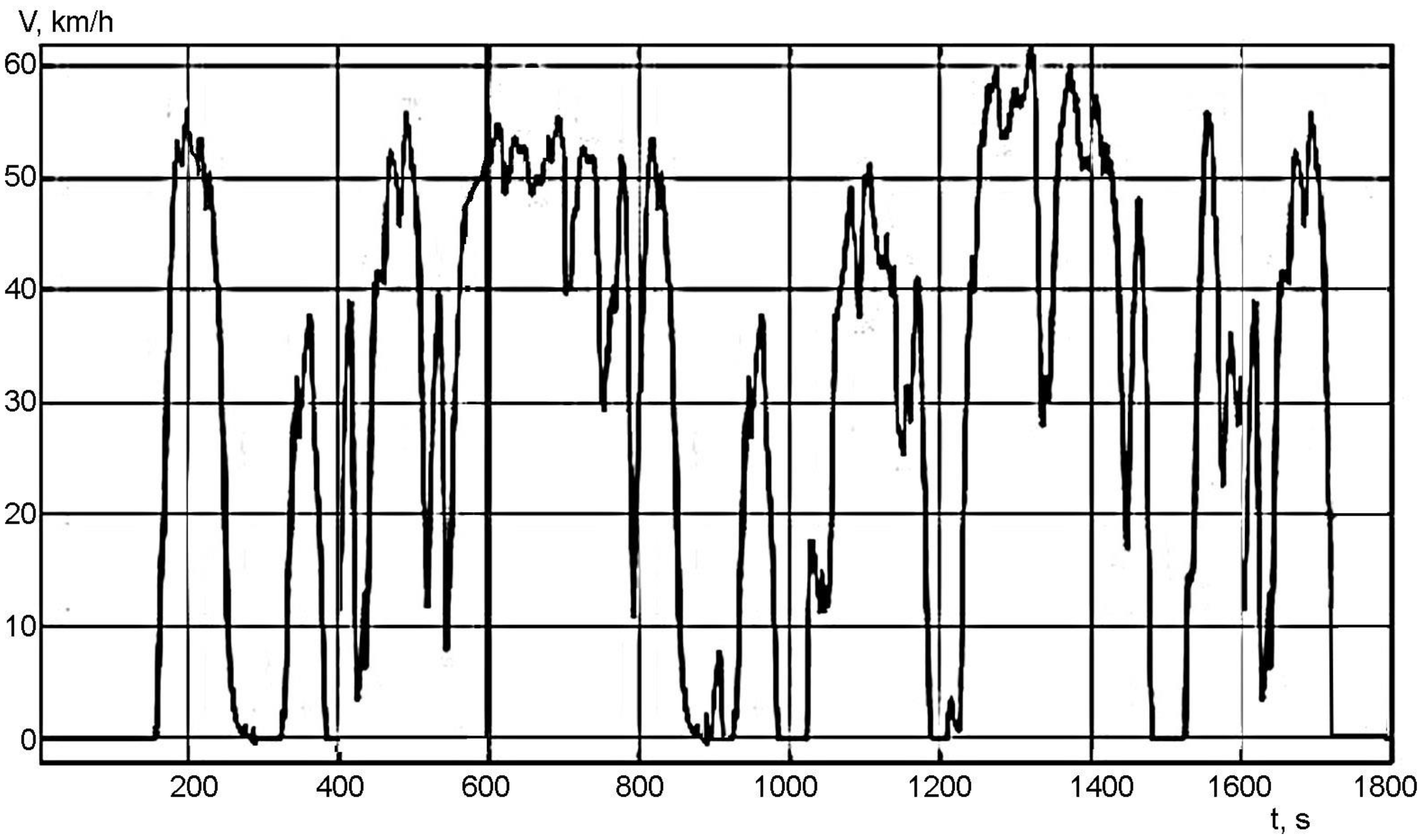
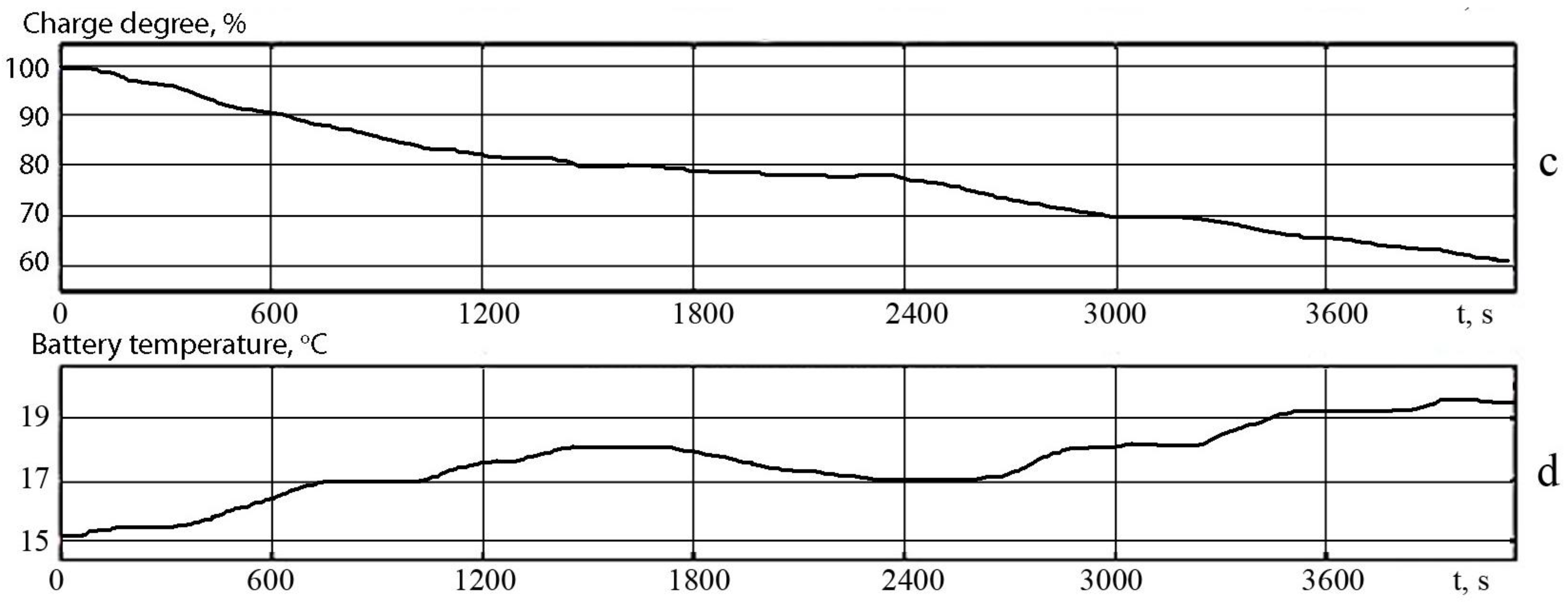
3. Obtaining the Initial Data for the Mathematical Model

In the course of experimental studies, to determine the depth of discharge of the battery, six races were made along predetermined routes. Each race assumed different road conditions and traffic intensity as well as vehicle loading.
The route includes both urban and suburban traffic modes. The maximum speed is 65 km/h; the electric car makes three stops for loading and unloading. During the experiment, 2 rides without load (10,000 kg) and 2 rides with partial load (16,000 kg) were carried out.
Measurements of electrical characteristics were carried out using CAN technology. At the same time, the following indicators were measured and recorded:
The degree of charge of the battery;
Torques of asynchronous electric motors;
Battery voltage;
Frequency of rotation of electric motors;
Temperature of electric motors and inverters.
The electric car has on board equipment that fixes the following specifications:
Ibatbattery current;
Pbatbattery power;
Ubatbattery voltage;
Efficiency is the efficiency of the system;
Wbat is the energy given off by the battery;
SOC is the degree of charge.
Characteristics are obtained using CAN bus communication technology and are recorded throughout the entire cycle.
The experiment was based on two routes that differ in traffic intensity and the amount of cycling of the lithium-ion battery.
On the first route, the electric car at the same time moved partially loaded, and the mass was 16,000 kg. Figure 1 shows a graph of the speed of an electric vehicle along route 1.
Figure 2 shows the characteristics of the traction electric drive system of an electric vehicle when driving along the first route.
The average battery current in the cycle was 140 A (0.7 C). The degree of charge decreased from 85 to 72 percent.
On the second route, the electric car moved partially loaded, and the mass was 16,000 kg. Figure 3 shows a graph of the speed of the electric vehicle along the second route.
Figure 4 shows the characteristics of the electric vehicle traction drive system. The average battery current in the cycle was 120 A (0.6 C). The degree of charge decreased from 72 to 54 percent. Table 1 shows the cycle parameters and energy characteristics. Unlike the abstract driving cycles often used in EV motion and performance simulations, these routes were derived from actual EV motion. This allows one to compare the real characteristics of the movement of the electric vehicles.
As a result of the tests, it was determined that the electric vehicle is capable of moving along the two routes under consideration with a fully charged battery, with a partial load. The depth of discharge was 20%.

4. Simulation of the Processes Occurring in the Battery during the Charge/Discharge Modes

For mathematical modeling of the processes of charge, discharge and charge transfer in the battery, a model of a separate battery was used, which reflects the following processes of energy conversion in the battery:
  • Processes of charge and discharge;
  • Processes of charge transfer between batteries in the battery;
  • Charge, discharge and charge transfer control processes.
When constructing equations relating the parameters of the mathematical model, the authors proposed an equivalent electrical circuit (Figure 5), which connects active and reactive elements, each of which imitates the physicochemical parameters of the battery under study or a structural element of an electrochemical battery [13].
The circuit is a series connection of an EMF source E m and four active resistances R 1 , R 2 , R p , R 0 . To take into account the inertia of the discharge/charge process parallel to the resistor R 1 included the electrical capacitance R 1 required to simulate transient processes when the load is turned on and off.
The characteristics of the battery for the purposes of this study are according to the manufacturer’s specification. The main characteristics of a single battery are:
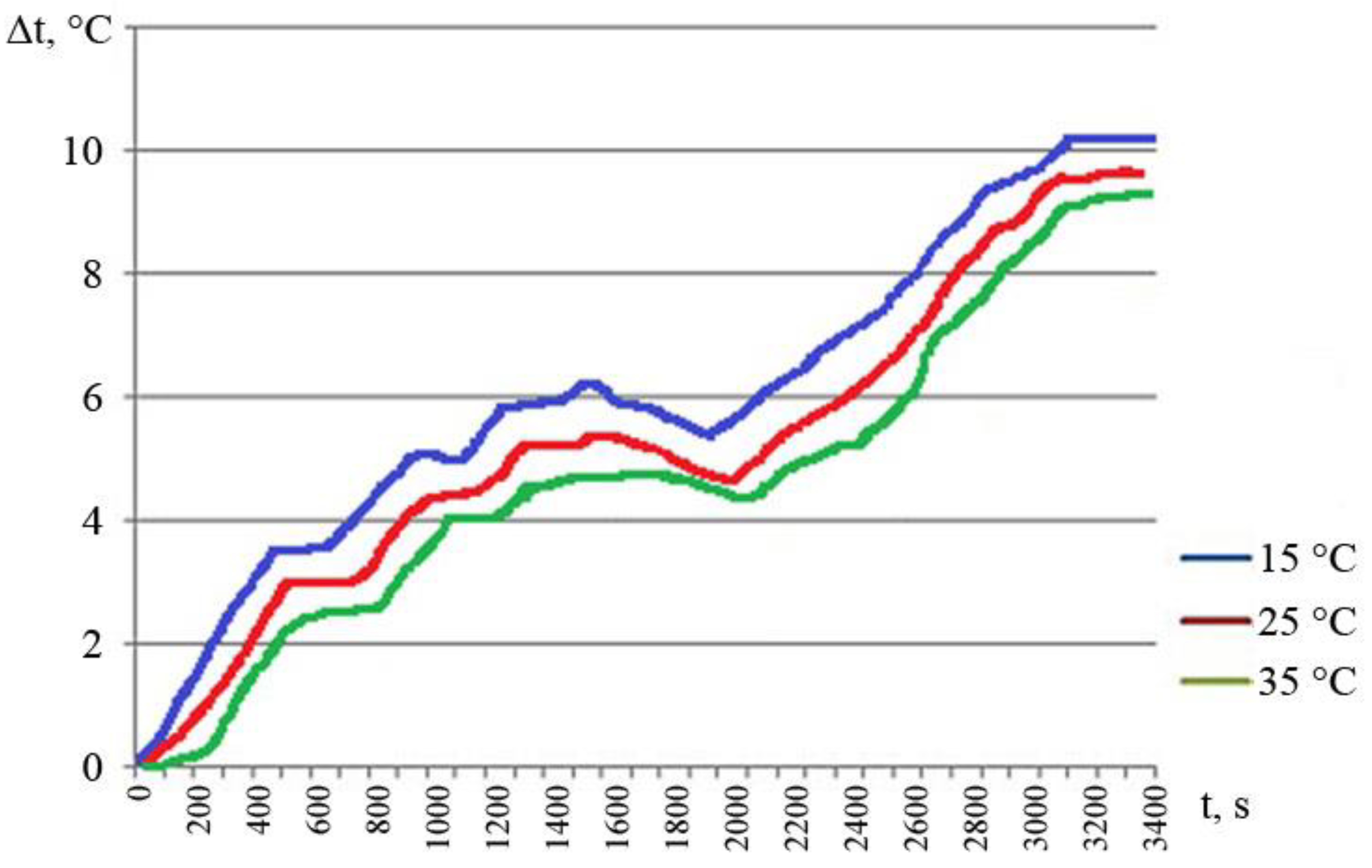
  • The chemical composition of the cathode material of the NMC battery (lithium-nickel-manganese-cobalt-oxide battery (LiNixMnyCozO2, NMC)—an alloy of nickel oxide, manganese, cobalt, and lithium;
  • Cell nominal voltage—3.8 V;
  • Lower voltage level 2.4 V;
  • The upper limit (depending on the charging or discharging process) of the battery open-circuit voltage is 4.2 V, at a temperature of 25 °C [14].
Below is the system of Equation (1) for the equivalent circuit of the battery shown in Figure 5. The mathematical model in this case is used to simulate the parameters of the battery, including the main branch, parasitic branch, capacity and electrolyte temperature:
E m = E m 0 K E ( 273 + θ ) ( 1 S O C ) R 1 = R 10 ln ( D O C ) C 1 = τ 1 R 1 R 2 = R 20 e ( A 21 ( 1 S O C ) ) 1 + e ( A 22 I m I * ) I p = V p n G p 0 e ( V p n ( V ρ s + 1 ) V ρ 0 + A ρ ( 1 θ θ ρ f ) ) Q e ( t ) = Q e _ i n i t + 0 t I m ( τ ) d r C ( I , θ ) = K c C 0 * K t 1 + ( K c 1 ) ( I I * ) δ S O C = 1 Q e C ( 0 , θ ) D O C = 1 Q e C ( I a v g , θ ) I a v g = I m ( τ 1 s + 1 ) θ ( t ) = θ e _ i n i t + 0 t ( P s θ θ α R θ ) C θ d τ P s = V R 1 2 R 1 + I 2 R 0 + I 2 R 2 R 0 = R 00 [ 1 + A 0 ( 1 S O C ) ] ]
The equivalent circuit depends on the battery current and nonlinear circuit elements. The above system of battery equations describes the components within the battery cell block. The system does not model the internal chemical processes of lithium-ion batteries directly—the equivalent circuit empirically approximately describes the processes occurring inside [15,16].
The equivalent circuit consists of two main parts: the main branch (elements R 1 C 1 , R 0 ), which approximately describes the dynamics of the battery under most conditions, and the parasitic branch R p , which describes the behavior of the battery at the end of the charge. The following is a detailed description of each of the circuit branches.
For the main branch, Equation (2) describes the internal electromotive force (EMF) or no-load voltage E m of one battery pack [17]. It is assumed that the value E m will be constant when the battery is fully charged. Voltage E m depends on temperature and battery state of charge (SOC) and is defined as follows:
E m = E m 0 K E ( 273 + θ ) ( 1 S O C )
where E m 0 is the no-load voltage at full charge, V; K E is the temperature coefficient, V/°C; θ is the electrolyte temperature, °C; S O C is the state of charge of the battery, p.u.
R 1 = R 10 ln ( D O C )
Equation (3) describes the change in resistance with charge depth. The resistance increases exponentially as the battery starts to exhaust itself during discharge [18].
The main resistance of the main branch is R 1 , where R 10 is constant, Ohm and D O C is the battery charge depth, r.u.
Equation (4) describes the transient process if the battery current has changed.
Capacity of the main branch C1:
C 1 = τ 1 R 1
where τ 1 = time constant of the main branch, s.
Resistance R 2 is determined by the formula
R 2 = R 20 e ( A 21 ( 1 S O C ) ) 1 + e ( A 22 I m I * )
where R 20 is resistance under normal conditions, Ohm; A 21 , A 22 are constants, r.u.; I m is the current of the main branch, A; I * is the current rated current of the battery, A.
The resistance across the terminals of one battery cell can be expressed as
R 0 = R 00 [ 1 + A 0 ( 1 S O C ) ]
where R 00 is resistance R0 with a completely infected battery (SOC = 1); A 0 is a constant determined by the accumulator parameters [19].
It is assumed that the resistance is constant at different temperatures and depends on the degree of charge [20].
The parasitic branch in the battery equivalent circuit consists of three components: a diode, resistance Rp of the parasitic branch, and a constant voltage source [21]. If the voltage across the diode exceeds the forward voltage Vpn, then the diode behaves as a linear resistor with a low resistance Rp. If the voltage across the diode is less than the forward voltage, then the diode behaves as a linear resistor with a low turn-off Gp. A constant voltage source maintains a constant voltage Vp0 at its output terminals regardless of the current flowing through the source. The output voltage is determined by the battery constant voltage parameter and can be any real value [22].
The value of the discharge current in the parasitic branch Ip is expressed by the dependence
I p = V p n G p 0 e ( V p n ( τ p s + 1 ) V ρ 0 + A ρ ( 1 θ θ ρ f ) )
where V p n is voltage on the parasitic branch, V; G p 0 is a constant determined by the accumulator parameters, s; τ p is the time constant of the parasitic branch, s; V ρ 0 is constant, V; Ap is constant, r.u.; θ is the electrolyte temperature, °C; θf is the freezing temperature of the electrolyte, °C.
Equation (7) describes parasitic current losses that occur during battery charging [22]. The current depends on the temperature of the electrolyte and the voltage of the parasitic branch. The current Ip is small under most conditions, with the exception of charging at high SOC [23]. It should be noted that the constant Gp0, as a rule, takes values greater than 1 s; the value of Gp0 is very small, on the order of 1012 s.
Equation (5) tracks the amount of charge drawn from the battery. It is determined by integrating the current flowing in the main branch in both directions, i.e., during battery charging and discharging [24]. Battery level Qe
Q e ( t ) = Q e _ i n i t 0 t I m ( t ) d t
where Qe_init is the initial value of the charge, A s; Im is the current in the main branch, A; t is the integration time variable, s.
Equation (9) describes the state of the battery capacity C based on the values of the discharge current and electrolyte temperature [25]:
C ( I , θ ) = K c C 0 * K t 1 + ( K c 1 ) ( I I * ) δ
where Kc is a constant; C0* is battery capacity without load at 0 °C, A s; Kt is the temperature coefficient; θ is the electrolyte temperature in °C; I is the discharge current in amperes; I* is the current rated current of the battery, A; δ is a constant determined by the accumulator parameters, r.u.
However, the dependence of capacitance on current is determined only during the discharge. During charging, the discharge current is set to zero in Equation (5) to calculate the total capacity [26].
Equations (10) and (11) describe the state of charge of the SOC and the depth of charge of the DOC of the battery. SOC determines the amount of remaining battery charge, and DOC determines the useful fraction of the remaining charge, taking into account the average discharge current. Large discharge currents cause a premature decrease in battery charge; thus, the DOC parameter is always less than or equal to the SOC parameter [27]:
S O C = 1 Q e C ( 0 , θ )
D O C = 1 Q e C ( I a v g , θ )
where Qe is the battery charge, A s; C is the battery capacity, A s; θ is the electrolyte temperature, °C; Iavg is the current average discharge current, A.
The current average discharge current Iavg is determined by the formula
I a v g = I m ( τ 1 s + 1 )
where Iavg is the current average discharge current, A; Im is the current of the main branch, A; τ 1 is the time constant of the main branch, s.
The change in temperature of the electrolyte in the battery θ is due to resistive losses Ps, taking into account the ambient temperature θa.
The thermal model consists of a first-order differential equation, with parameters for thermal resistance and capacitance:
θ ( t ) = θ e _ i n i t + 0 t ( P s θ θ α R θ ) C θ d τ
where θa is the ambient air temperature, °C; θinit is the initial temperature of the battery (assumed to be equal to the ambient air temperature), °C; Cθ is the thermal capacity, J/°C; τ is the integration time variable, s; Rθ is the thermal resistance, °C/W; t is the simulation time, s; Ps is the power loss at active resistances R from R0 and R2, W.
P s = V R 1 2 R 1 + I 2 R 0 + I 2 R 2
The power loss Ps is the heat loss power with which the battery heating can be calculated. On the basis of the described mathematical equations, a mathematical model will be further formed, which allows taking into account the processes occurring in the battery and taking into account the current profile [28].
The simulation and solution were obtained using the Matlab program (Appendix A). In the section Appendix A.1, we provide a description of the block diagram of the mathematical model in Matlab, the data that we used in the model, the basic equations of the blocks and the implementation of the thermal model in the Matlab program.
In the section Appendix A.2, we provide a logic diagram for switching motion cycles, as well as a charge cycle.

5. Discussion

One of the main criteria for optimizing battery life is temperature. As mentioned earlier, battery operation at low temperatures leads to a sharp decrease in the number of cycles. At positive temperatures, the recommended operating range is 10–35 °C. During the operating mode, the walls of the battery are heated. To determine the temperature after the operation cycle, it is necessary to carry out mathematical modeling. The current profile during a driving cycle on route 1 is reduced to one battery by dividing the total current by the number of cells connected in parallel (Figure 6).
The results of modeling the main characteristics of the battery at an ambient temperature of 15 °C are shown in Figure 6.
The maximum heating of the battery was 25 °C after a driving cycle on routes 1 and 2. The difference between the initial temperature and the temperature at the end of the cycle was 50 °C. The degree of charge decreased from 100% to 60%. The battery voltage dropped to 3.6 V.
Similar studies were carried out for 25 and 35 degrees, respectively, as the most typical operating temperatures for traction batteries. The results are shown in Figure 7 and Figure 8.
As can be seen from the graph, the heating for the cycle was 29.2 °C, and the difference between the initial temperature and the temperature at the end of the cycle was 4.2 °C. This is due to the decrease in internal resistance as the temperature of the battery rises. Another calculation was made at an ambient temperature of 35 °C. This temperature range is critical for the battery; the resource under such conditions is significantly reduced. At an initial temperature of 40 °C, the heating per cycle was 39 °C, and the difference between the initial temperature of the cell and the temperature at the end of the cycle was 4 °C (Figure 9).
The results obtained show the heating of the battery in the absence of air conditioning in the cooling system. Figure 9 shows the temperature difference achieved by the battery when alternating routes 1 and 2.

6. Conclusions

Based on the battery equivalent circuit and the system of equations, a simulation model was created to calculate the electrical and thermal characteristics. The equivalent circuit includes active and reactive elements, each of which imitates the physicochemical parameter of the battery under study or the structural element of the electrochemical battery.
The input signals of the mathematical model are the current and ambient temperatures obtained during the tests of the electric vehicle, and the output signals are the voltage, electrolyte temperature and degree of charge. The resulting equations make it possible to assign values of internal resistance to a certain temperature value and a certain value of the degree of charge.
As a result of simulation modeling, the heating of the battery was determined at various values of the ambient temperature. It was found that at an ambient temperature of 20 °C, the heating at the end of the cycle was 25 °C; at 30 °C, the same parameter took on a value of 4.2 °C; and at 35 °C was 4 °C.
The absence of a forced cooling system in the model makes it possible to determine the degree of heating not only of the outer walls of the accumulator, but also inside the cell. When the charge/discharge cycle is continuous, the temperature of the element does not fall to its original state but, on the contrary, continues to increase. When determining battery life, a temperature range of more than 45 °C is not calculated, as battery life is significantly reduced. As a result of simulation modeling, a tool was obtained for calculating battery heating under various environmental conditions. During operation, the maximum heating will not exceed 50 °C, which allows us to conclude that the range recommended for battery operation will be provided.
The simulation results will be useful to researchers and developers of autonomous power sources for electric vehicles and other devices for the implementation of real-time systems that take into account the processes of changing the characteristics of traction batteries. The developed mathematical model can be used in battery management systems to monitor the state of charge and battery degradation using the assessment of the state of charge (SOC) and the state of health (SOH). This is especially important when designing and operating a smart battery management system (BMS) in virtually any lithium-ion battery application, providing information about how long the device will run before it needs to be charged (SOC value) and when the battery should be replaced due to loss of battery capacity (SOH value). Based on the equivalent circuit of the battery and the system of equations, a simulation model was created to calculate the electrical and thermal characteristics.

Author Contributions

Conceptualization, B.V.M. and N.V.M.; methodology, S.N.S. and E.A.E.; software, M.Q.; validation, S.N.S. and B.V.M.; formal analysis, N.V.M.; investigation, E.A.E.; resources, E.A.E.; data curation, S.N.S.; writing—original draft preparation, B.V.M.; writing—review and editing, N.V.M.; visualization, M.Q. All authors have read and agreed to the published version of the manuscript.

Funding

This research received no external funding.

Institutional Review Board Statement

Not applicable.

Informed Consent Statement

Not applicable.

Data Availability Statement

The data presented in this study are available from the corresponding authors upon reasonable request.

Conflicts of Interest

The authors declare no conflict of interest.

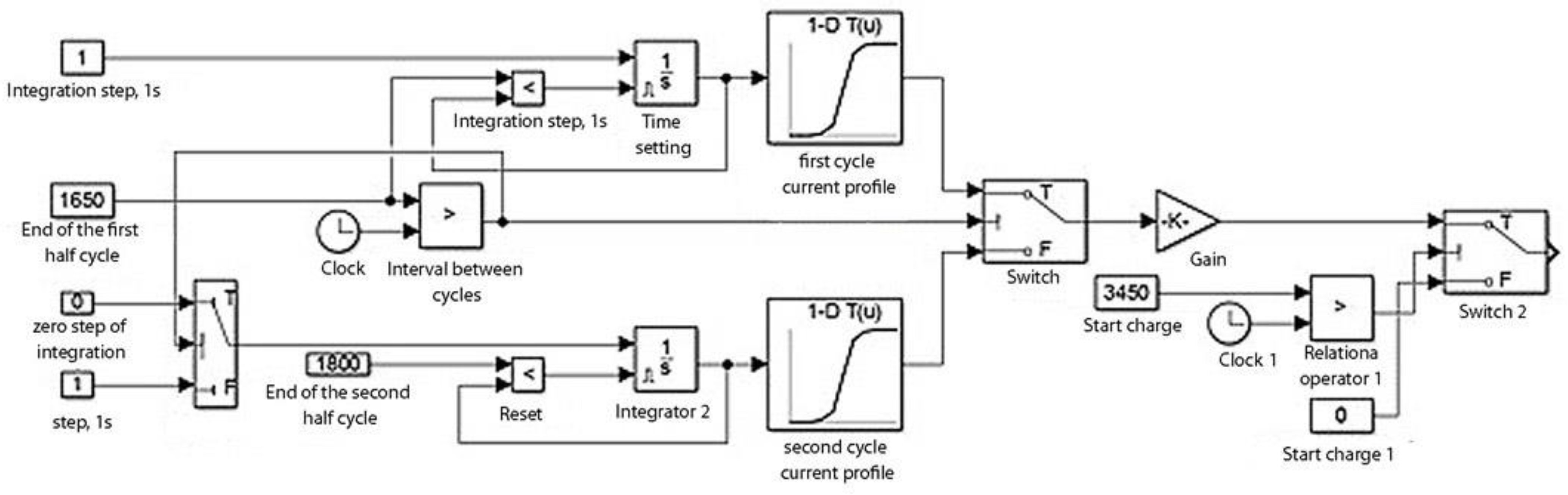
Appendix A. Modeling Blocks and Data Used in the Matlab Program

Appendix A.1. Block Diagram of the Mathematical Model of the Battery

In this section, we provide a description of the block diagram of the mathematical model in Matlab, the data that we used in the model, the basic equations of the blocks, and the implementation of the thermal model in the Matlab program.
The mathematical model of processes in the battery was developed in Matlab (Figure A1). The capacitance model calculates the state of charge (SOC) and depth of charge of the battery, the voltage model calculates the resistance as a function of the state of charge and the depth of charge, and the thermal model calculates the internal temperature [29].
The input signals of the mathematical model are current and ambient temperature, and the output signals are voltage, electrolyte temperature and degree of charge [30].
Figure A1. Block diagram of the mathematical model in Matlab.
Mathematics 11 00536 g0a1
The description of the blocks of the mathematical model of the battery is presented below.
Em_Table—EMF source, its input and output parameters:
inputs
T = {293.15,’K’} % T:right
end
outputs
C = {31,’A*hr’} %C:left
SOC = {1,’1’} %SOC:left
end
Basic Block Equations:
equations
% Charge deficit calculation, preventing SOC > 1
If Qe < 0 && i > 0 Qe.der == 0;
else Qe.der == -i;
end
% Perform the capacity table lookup C == tablelookup(Temp_Table,C_Table,T,...
interpolation = linear,extrapolation = nearest)
% SOC Equation SOC == 1–Qe/C;
% Electrical equation by table lookup v == tablelookup(SOC_Table,Temp_Table,Em_Table,SOC,T,...
interpolation = linear,extrapolation = nearest)
end
Block C1—equivalent capacitance of the RC circuit, input and output parameters:
inputs
T = {293.15,’K’}; %T:left SOC = {1,’1’}; %SOC:left
end
parameters (Size = variable) C_Table = {ones(5,3),’F’}
% Matrix of capacitance values, C(SOC,T) SOC_Table = {[0;0.1;0.5;0.9;1],’1 ‘} % State of charge (SOC) breakpoints Temp_Table = {[273.15 293.15 313.15],’K’} % Temperature (T) breakpoints
end
Block equations:
equations let
% Perform the table lookup C =
tablelookup(SOC_Table,Temp_Table,C_Table,SOC,T,...
interpolation = linear,extrapolation = nearest)
in
% Electrical equation i == C * v.der; end end
Block R1—equivalent resistance of the RC circuit, input and output parameters:
inputs
T = {293.15,’K’}; %T:left SOC = {1,’1’}; %SOC:left
end
outputs pow = {0,’W’}; %POW:right
end
Block Equations:
let
% Perform the table lookup
R = tablelookup(SOC_Table,Temp_Table,R_Table,SOC,T,…
interpolation = linear,extrapolation = nearest)
in
% Electrical Equations
v == i*R; pow == v*i;
end
end
Block R0 is equivalent internal resistance; input and output parameters are similar to block R1.
The resulting equations allow for assigning internal resistance values to a certain temperature value and a certain value of the degree of charge (Table A1).
Table A1. Parameters of a typical lithium-ion battery based on NMC technology.
Cell Temperature0 °C30 °C45 °CState of Charge (SZ), %
Available battery capacity18.00817.62517.639
Battery voltage at different states of charge2.522.732.540
2.632.822.4510
2.873.123.2125
3.393.513.5450
3.713.93.9175
44490
4.14.24.31100
Figure A2 shows a graph of the open-circuit voltage versus the battery state of charge.
Figure A2. Battery open-circuit voltage (OCV).
Mathematics 11 00536 g0a2
In order to apply the TAB current obtained during the operation of the electric vehicle to the input, it is necessary to form data tables in which the values of the currents in the cycle will be indicated, depending on the time. In addition, a full cycle of movement along the route provides for one stop after passing the halfway point.
The thermal model block represents a thermal model that contains a heat source, a temperature sensor and a battery mass; see Figure A3.
Figure A3. Thermal model in the MATLAB program.
Mathematics 11 00536 g0a3
The description of the blocks is given for the thermal model below:
inputs
S = { 0, ‘K’ }; %S:bottom
end nodes
A = foundation.thermal.thermal; %A:bottom B = foundation.thermal.thermal; %B:top
end
variables (Access = private) Q = { 0, ‘J/s’ }; T = { 0, ‘K’ };
end branches
Q : BQ -> AQ;
end equations
T == BT–AT;
T == S;
end
end
The thermal model allows for calculating the heating of the battery, the air intake for cooling of which is carried out directly from the environment. The ambient temperature corresponds to the temperature of the interaction of the battery walls with the air of the cooling system. When using an air conditioner in the cooling system, the temperature of the blown air will correspond to the temperature of the conditioned air. In this case, the airflow rate must be selected in accordance with the power and operating mode of the compressor. In this work, the flow rate was not taken into account; this allows one to more accurately determine the temperature inside the cell, because there is no forced heat extraction. Based on the obtained mathematical model, data on the heat release of the battery cell in the motion cycle are calculated [31].

Appendix A.2. Modeling Blocks of the Charge/Discharge Modes of an Electric Vehicle Battery

We provide a logic diagram for switching motion cycles, as well as a charge cycle. To simulate the load cycle of the battery, it is necessary to set the alternation of several charge/discharge modes in accordance with the routes of the electric vehicle. The alternation of cycles is necessary to determine the time intervals during which it is necessary to charge the battery. With the help of the alternation of motion cycles, the heating and the depth of discharge of the battery are determined [32]. When the set depth of discharge is reached, the battery is charged with the rated current. These algorithms will allow simulating the movement of an electric vehicle, taking into account a fast charge at the final stops, as well as choosing the best option for installing charging stations along the route to improve the battery resource [33]. The logic diagram for switching between cycles is shown in Figure A4.
Figure A4. Logic diagram for switching motion cycles, as well as the charge cycle.
Mathematics 11 00536 g0a4
The logical scheme presents two main cycles, according to which the calculation of battery modes is performed. The current profiles correspond to the first and second routes.
The formation of time intervals can be done using the “clock” block, but if the cycles alternate one after the other, a timer must be used. The timer consists of an integrator block whose step is one second (Figure A5).
Figure A5. Forming a timer in Matlab.
Mathematics 11 00536 g0a5
The block also contains a counter reset, the input of which accepts a logical zero and a logical one, in the case of setting the reset of the counter for the time interval for which the battery is discharged. The exit from the time setting block is compared with the required end time of the first cycle (end of the first and second route).
In the logic diagram, the battery charge current and the duration of its operation can be configured. In the real tests, the charge was formed after two complete cycles of movement.

References

  1. Waldmann, T.; Kasper, M.; Fleischhammer, M.; Wohlfahrt-Mehrens, M. Temperature dependent aging mechanisms in Lithium—Ion batteries—A Post—Mortem study. J. Power Sources 2014, 363, 129–135. [Google Scholar] [CrossRef]
  2. Isametova, M.E.; Nussipali, R.; Martyushev, N.V.; Malozyomov, B.V.; Efremenkov, E.A.; Isametov, A. Mathematical Modeling of the Reliability of Polymer Composite Materials. Mathematics 2022, 10, 3978. [Google Scholar] [CrossRef]
  3. Xia, B.; Wang, S.; Tian, Y.; Sun, W.; Xu, Z.; Zheng, W. Experimental research on the linixcoymnzo2 lithium-ion battery characteristics for model modification of SOC estimation. Inf. Technol. J. 2014, 13, 2395–2403. [Google Scholar] [CrossRef] [Green Version]
  4. Shchurov, N.I.; Myatezh, S.V.; Malozyomov, B.V.; Shtang, A.A.; Martyushev, N.V.; Klyuev, R.V.; Dedov, S.I. Determination of Inactive Powers in a Single-Phase AC Network. Energies 2021, 14, 4814. [Google Scholar] [CrossRef]
  5. Li, X.; Jiang, J.; Zhang, C.; Wang, L.Y.; Zheng, L. Robustness of SOC estimation algorithms for EV lithium-ion batteries against modeling errors and measurement noise. Math. Probl. Eng. 2015, 2015, 719490. [Google Scholar] [CrossRef] [Green Version]
  6. Tian, Y.; Xia, B.; Wang, M.; Sun, W.; Xu, Z. Comparison study on two model-based adaptive algorithms for SOC estimation of lithium-ion batteries in electric vehicles. Energies 2014, 7, 8446–8464. [Google Scholar] [CrossRef] [Green Version]
  7. Tseng, K.-H.; Liang, J.-W.; Chang, W.; Huang, S.-C. Regression models using fully discharged voltage and internal resistance for state of health estimation of lithium-ion batteries. Energies 2015, 8, 2889–2907. [Google Scholar] [CrossRef] [Green Version]
  8. Shchurov, N.I.; Dedov, S.I.; Malozyomov, B.V.; Shtang, A.A.; Martyushev, N.V.; Klyuev, R.V.; Andriashin, S.N. Degradation of Lithium-Ion Batteries in an Electric Transport Complex. Energies 2021, 14, 8072. [Google Scholar] [CrossRef]
  9. Hafsaoui, J.; Sellier, F. Electrochemical model and its parameters identification tool for the follow up of batteries aging. World Electric. Veh. J. 2010, 4, 386–395. [Google Scholar] [CrossRef]
  10. Prada, E.; Di Domenico, D.; Creff, Y.; Sauvant-Moynot, V. Towards advanced BMS algorithms development for (p)hev and EV by use of a physics-based model of Li-Ion Battery Systems. World Electric. Veh. J. 2013, 6, 807–818. [Google Scholar] [CrossRef]
  11. Varini, M.; Campana, P.E.; Lindbergh, G. A semi-empirical, electrochemistry-based model for Li-ion battery performance prediction over lifetime. J. Energy Storage 2019, 25, 100819. [Google Scholar] [CrossRef]
  12. Ashwin, T.R.; McGordon, A.; Jennings, P.A. Electrochemical modeling of li-ion battery pack with constant voltage cycling. J. Power Sources 2017, 341, 327–339. [Google Scholar] [CrossRef]
  13. Somakettarin, N.; Pichetjamroen, A. A study on modeling of effective series resistance for lithium-ion batteries under life cycle consideration. IOP Conf. Ser. Earth Environ. Sci. 2019, 322, 012008. [Google Scholar] [CrossRef]
  14. Kuo, T.J.; Lee, K.Y.; Chiang, M.H. Development of a neural network model for SOH of LiFePO4 batteries under different aging conditions. IOP Conf. Ser. Mater. Sci. Eng. 2019, 486, 012083. [Google Scholar] [CrossRef]
  15. Davydenko, L.; Davydenko, N.; Bosak, A.; Bosak, A.; Deja, A.; Dzhuguryan, T. Smart Sustainable Freight Transport for a City Multi-Floor Manufacturing Cluster: A Framework of the Energy Efficiency Monitoring of Electric Vehicle Fleet Charging. Energies 2022, 15, 3780. [Google Scholar] [CrossRef]
  16. Mamun, K.A.; Islam, F.R.; Haque, R.; Chand, A.A.; Prasad, K.A.; Goundar, K.K.; Prakash, K.; Maharaj, S. Systematic Modeling and Analysis of On-Board Vehicle Integrated Novel Hybrid Renewable Energy System with Storage for Electric Vehicles. Sustainability 2022, 14, 2538. [Google Scholar] [CrossRef]
  17. Chao, P.-P.; Zhang, R.-Y.; Wang, Y.-D.; Tang, H.; Dai, H.-L. Warning model of new energy vehicle under improving time-to-rollover with neural network. Meas. Control. 2022, 55, 1004–1015. [Google Scholar] [CrossRef]
  18. Pusztai, Z.; K’orös, P.; Szauter, F.; Friedler, F. Vehicle Model-Based Driving Strategy Optimization for Lightweight Vehicle. Energies 2022, 15, 3631. [Google Scholar] [CrossRef]
  19. Mariani, V.; Rizzo, G.; Tiano, F.; Glielmo, L. A model predictive control scheme for regenerative braking in vehicles with hybridized architectures via aftermarket kits. Control Eng. Pract. 2022, 123, 105142. [Google Scholar] [CrossRef]
  20. Hensher, D.A.; Wei, E.; Liu, W. Battery electric vehicles in cities: Measurement of some impacts on traffic and government revenue recovery. J. Transp. Geogr. 2021, 94, 103121. [Google Scholar] [CrossRef]
  21. Li, S.; Yu, B.; Feng, X. Research on braking energy recovery strategy of electric vehicle based on ECE regulation and I curve. Sci. Prog. 2020, 103, 0036850419877762. [Google Scholar] [CrossRef] [PubMed]
  22. Laadjal, K.; Cardoso, A.J.M. Estimation of Lithium-Ion Batteries State-Condition in Electric Vehicle Applications: Issues and State of the Art. Electronics 2021, 10, 1588. [Google Scholar] [CrossRef]
  23. Arango, I.; Lopez, C.; Ceren, A. Improving the Autonomy of a Mid-Drive Motor Electric Bicycle Based on System Efficiency Maps and Its Performance. World Electric. Veh. J. 2021, 12, 59. [Google Scholar] [CrossRef]
  24. Mei, J.; Zuo, Y.; Lee, C.H.; Wang, X.; Kirtley, J.L. Stochastic optimization of multi-energy system operation considering hydrogen-based vehicle applications. Adv. Appl. Energy 2021, 2, 100031. [Google Scholar] [CrossRef]
  25. Wu, X. Research and Implementation of Electric Vehicle Braking Energy Recovery System Based on Computer. J. Phys. Conf. Ser. 2021, 1744, 022080. [Google Scholar] [CrossRef]
  26. Istomin, S. Development of a system for electric power consumption control by electric rolling stock on traction tracks of locomotive depots. IOP Conf. Ser. Mater. Sci. Eng. 2020, 918, 012157. [Google Scholar] [CrossRef]
  27. Domanov, K.; Shatohin, A.; Nezevak, V.; Cheremisin, V. Improving the technology of operating electric locomotives using electric power storage device. E3S Web Conf. 2019, 110, 01033. [Google Scholar] [CrossRef]
  28. Debelov, V.V.; Endachev, D.V.; Yakunov, D.M.; Deev, O.M. Charging balance management technology for low-voltage battery in the car control unit with combined power system. IOP Conf. Ser. Mater. Sci. Eng. 2019, 534, 012029. [Google Scholar] [CrossRef]
  29. Widmer, F.; Ritter, A.; Duhr, P.; Onder, C.H. Battery lifetime extension through optimal design and control of traction and heating systems in hybrid drivetrains. ETransportation 2022, 14, 100196. [Google Scholar] [CrossRef]
  30. Liu, X.; Zhao, M.; Wei, Z.; Lu, M. The energy management and economic optimization scheduling of microgrid based on Colored Petri net and Quantum-PSO algorithm. Sustain. Energy Technol. Assess. 2022, 53, 102670. [Google Scholar] [CrossRef]
  31. Tormos, B.; Pla, B.; Bares, P.; Pinto, D. Energy Management of Hybrid Electric Urban Bus by Off-Line Dynamic Programming Optimization and One-Step Look-Ahead Rollout. Appl. Sci. 2022, 12, 4474. [Google Scholar] [CrossRef]
  32. Zhou, J.; Feng, C.; Su, Q.; Jiang, S.; Fan, Z.; Ruan, J.; Sun, S.; Hu, L. The Multi-Objective Optimization of Powertrain Design and Energy Management Strategy for Fuel Cell–Battery Electric Vehicle. Sustainability 2022, 14, 6320. [Google Scholar] [CrossRef]
  33. Martyushev, N.V.; Malozyomov, B.V.; Khalikov, I.H.; Kukartsev, V.A.; Kukartsev, V.V.; Tynchenko, V.S.; Tynchenko, Y.A.; Qi, M. Review of Methods for Improving the Energy Efficiency of Electrified Ground Transport by Optimizing Battery Consumption. Energies 2023, 16, 729. [Google Scholar] [CrossRef]
Figure 1. Dependence of speed on time on the first route.
Mathematics 11 00536 g001
Figure 2. Energy characteristics of the electric vehicle of the first route: (a) Ibat is the battery current; (b) Ubat is the battery voltage; (c) SOC is the degree of charge; (d) Pbat is the battery power; (e) Wbat is the energy given off by the battery; (f) efficiency is the efficiency of the system.
Mathematics 11 00536 g002
Figure 3. The graph of the change in the speed of an electric vehicle depending on the time along the second route.
Mathematics 11 00536 g003
Figure 4. Energy characteristics of the electric vehicle of the second route: (a) Ibat is the battery current; (b) Ubat is the battery voltage; (c) SOC is the degree of charge; (d) Pbat is the battery power; (e) Wbat is the energy given off by the battery; (f) efficiency is the efficiency of the system.
Mathematics 11 00536 g004
Figure 5. Equivalent electrical circuit of the model of the electrochemical cell of the battery.
Mathematics 11 00536 g005
Figure 6. Time waveforms of the main characteristics of the battery in cycles at an ambient temperature of 15 °C: (a) battery discharge/charge current; (b) voltage of battery; (c) battery charge degree; (d) battery temperature.
Mathematics 11 00536 g006aMathematics 11 00536 g006b
Figure 7. Graphs of the main characteristics of the battery in cycles at an ambient temperature of 25 °C: (a) battery discharge/charge current; (b) voltage of battery; (c) battery charge degree; (d) battery temperature.
Mathematics 11 00536 g007aMathematics 11 00536 g007b
Figure 8. Graphs of the main characteristics of the battery in cycles at an ambient temperature of 35 °C: (a) battery discharge/charge current; (b) voltage of battery; (c) battery charge degree; (d) battery temperature.
Mathematics 11 00536 g008
Figure 9. Battery heating at different ambient temperatures.
Mathematics 11 00536 g009
Table 1. Control cycle parameters and test results electric vehicle.
RouteDistance, kmAverage Speed, km/hEnergy in the Cycle, kWRecovery Energy, kWhEnergy
Consumption, kW∙h/km
First route12.9534.8513.93.111.11
Second route16.127.6622.442.941.38
Disclaimer/Publisher’s Note: The statements, opinions and data contained in all publications are solely those of the individual author(s) and contributor(s) and not of MDPI and/or the editor(s). MDPI and/or the editor(s) disclaim responsibility for any injury to people or property resulting from any ideas, methods, instructions or products referred to in the content.

