Adaptive Load Incremental Step in Large Increment Method for Elastoplastic Problems

Abstract

As a force-based finite element method (FEM), large increment method (LIM) shows unique advantages in material nonlinearity problems. In LIM for material nonlinearity analysis, adaptive load incremental step is a fundamental step for its successful application. In this work, a strategy to automatically refine the load incremental step is proposed in the framework of LIM. The adaptive load incremental step is an iterative process based on the whole loading process, and the location and number of post-refined incremental steps are determined by the posteriori error of energy on the pre-refined incremental steps. Furthermore, the iterative results from the pre-refined incremental steps can be utilized as the initial value to calculate the result for the post-refined incremental steps, which would significantly improve the computational accuracy and efficiency. The strategy is demonstrated using a two-dimensional example with a bilinear hardening material model under cyclic loading, which verifies the accuracy and efficiency of the strategy in LIM. Compared with the displacement-based FEM, which relies upon a step-by-step incremental approach stemming from flow theory, the adaptive load incremental step based on the whole loading process of LIM can avoid the cumulative errors caused by step-by-step in global stage and can quantify the accuracy of results. This work provides a guidance for the practical application of LIM in nonlinear problems.

1. Introduction

The finite element method (FEM) is a powerful numerical method to solve approximate solution of problems and has been widely used in many areas of engineering [1,2,3,4,5]. Material nonlinearity problems involve a history-dependent response, and therefore, a series of increments are usually conducted in FEM to solve these problems [6,7]. Most commonly, the choice of increment number and size have a significant effect on the accuracy and convergence of results [8]. To avoid the influence of artificially selected incremental steps on the result accuracy, the adaptive load incremental step has been introduced in FEM [9,10,11].

Based on the main unknown variables, FEM has been divided into two categories; the displacement-based method [12,13] and the force-based method [14,15]. For elastoplastic problems, the displacement-based FEM relies upon a step-by-step incremental approach at a global (system) stage stemming from flow theory [6,7], and its system equations at the global stage is changing with material nonlinearity, thus, the error accumulation and computational inefficiencies are still challenging problems. Based on the theory of the displacement-based FEM frame, the adaptive load increment step is achieved by automatically adjusting the size of each step in sequence [9,10,11]. The above shortcomings still exist. Thus, some researchers re-resorted to the force-based FEM [14,15,16,17]. As a typical force-based FEM, the large increment method (LIM) has some unique advantages for elastoplastic problems [15]. In LIM, the equations are separated into the global stage equilibrium and compatibility equations and the local (element) stage physical equations. Thus, the material nonlinearity is treated at the local stage, separately. Moreover, the global equilibrium and compatibility equations remain consistent during the whole loading process in the case of small deformation. Owing to these features, for elastoplastic problems, an overall iterative process in the local stage is implemented to obtain final results in LIM. Thus, based on the features of LIM in dealing with material nonlinearity in the local stage and the consistent global equilibrium and compatibility equations, the computational inefficiencies and error accumulation of results caused by the step-by-step process at the global stage of FEM can be impressed, and thus, further exploring the adaptive load incremental step strategy in LIM constitutes valuable research.

LIM was proposed by Zhang and Liu [15] for material nonlinear problems. In recent years, LIM has been extended for solving truss and beam structures [18,19,20,21] and 2D and 3D continua [14,15,22,23,24,25] with nonlinear materials under monotonic and cycle loading [14,15,18,19,20,21,24,25,26]. These works have proved that LIM has great advantages and shows a good application prospect for material nonlinear problems. For elastoplastic problems, the allocation of the incremental steps on the whole loading process has a significant effect on the accuracy of results and computational efficiency. In previous studies [14,15,18,21,23,26], the incremental steps were selected evenly on the loading process for simplicity. In this case, two shortcomings have been observed as follows: (1) incremental steps cannot be rationally allocated to ensure the accuracy of results and the computational efficiency, and (2) the accuracy of the results can hardly be quantitatively evaluated. The location of the adaptive load incremental steps can be automatically adjusted according to the quantification of impact of each step on the results, and the desired accuracy can be obtained with as little computation cost as possible. Therefore, an adaptive load incremental step strategy and a quantification estimation method in LIM need to be explored.

To this end, this paper proposes an adaptive load incremental step strategy in LIM for elastoplastic material problems based on the posteriori error estimation of energy. The strategy in LIM can avoid the error accumulation caused by the step-by-step process at the global stage and can quantify the accuracy of results. Before proposing the adaptive load incremental step strategy, the procedure of LIM for elastoplastic material problems is described in Section 2. Then, the posteriori error estimation of energy and the adaptive load incremental step procedure are discussed. Furthermore, a numerical example with bilinear hardening material under cyclic loading is presented to validate the proposed strategy. Finally, the conclusions are drawn.

2. LIM for Elastoplastic Material Problems

As the foundation, the procedure of LIM for elastoplastic material problems is briefly described in this section. More details on LIM can be found in works of Liu et al. [15,19,23].

2.1. Governing Equations in LIM

For a continuum body Ω, its boundary is represented as ∂Ω. The continuum body is subjected to the body force f in Ω, and the external force t is exerted on the boundary ∂Ω. The continuum body is divided into finite elements. The stress σ and displacement u at each point in any element Ω^e can be expressed in terms of the element generalized force variables and element nodal displacement variables. In each element, the stress vector σ can be represented as [18,19]

$$\sigma =Z{F}^e,$$

(1)

where Z is the stress shape function and F^e is the elemental generalized inner forces (an m-dimensional vector). The displacement field is same as the displacement-based finite element method [2], and the displacement field in each element can be written as

$$u=N{d}^{\mathrm{e}},$$

(2)

where u is the displacement vector, N is the displacement shape function, and d^e denotes the nodal displacement (an n-dimensional vector). The strain vector ε in each element is obtained as

$$\mathsf{\epsilon }=Lu=LN{d}^{\mathrm{e}}=B{d}^{\mathrm{e}},$$

(3)

where L is the differential operator, and B is the strain-displacement matrix in element.

Using the principle of virtual work in an element domain Ω^e, the equilibrium equations are represented as

$${\displaystyle {\int }_{{\mathsf{\Omega }}^{\mathrm{e}}}\mathsf{\sigma }\delta \mathsf{\epsilon } \mathrm{d}\Omega }={\displaystyle {\int }_{{\mathsf{\Omega }}^{\mathrm{e}}}f\delta u \mathrm{d}\mathsf{\Omega }}+{\displaystyle {\int }_{\partial {\mathsf{\Omega }}^{\mathrm{e}}}t\delta u \mathrm{dS}},$$

(4)

where f and t are the body force in Ω^e and the surface force on ∂Ω^e, respectively, and δε and δu are the virtual strain and virtual displacement, respectively. Substituting Equations (1) and (3) into Equation (4), the element equilibrium equations can be derived as [15]

$$C^{\mathrm{e}}{F}^{\mathrm{e}}=P^{\mathrm{e}},$$

(5)

where the elemental equilibrium matrix C^e and the equivalent force vector of the element P^e are

$$C^{\mathrm{e}}={\displaystyle {\int }_{{\mathsf{\Omega }}^{\mathrm{e}}}{B}^{\mathrm{T}}Z \mathrm{d}}\mathsf{\Omega },$$

(6)

and

$$P^{\mathrm{e}}={\displaystyle {\int }_{{\mathsf{\Omega }}^{\mathrm{e}}}{N}^{\mathrm{T}}f \mathrm{d}\mathsf{\Omega }}+{\displaystyle {\int }_{\partial {\mathsf{\Omega }}^{\mathrm{e}}}{N}^{\mathrm{T}}t \mathrm{dS}},$$

(7)

respectively. The equilibrium equations of the system are obtained by assembling all the elemental equilibrium matrices as [15]

$$CF=P,$$

(8)

where C is the equilibrium matrix of the system, F is the generalized inner force vector of the system, and P is the external load vector. The equilibrium matrix C is an M × N matrix (M ≤ N), where M is the degree of freedom of the system, and N is the number of unknown generalized inner forces of the system. For a statically determinate system, the equilibrium matrix C is a square matrix with M = N, the generalized inner force vector F can be obtained directly by the full rank linear equations in Equation (8). However, the system is usually statically indeterminate. In this case, the equilibrium matrix C of is a non-square matrix with M < N, and the equilibrium equations are not enough to determine the generalized inner force vector F.

For the statically indeterminate system, the compatibility condition is considered. According to the principle of complementary virtual work and using the Equations (1) and (3), there is

$${\displaystyle {\int }_{{\mathsf{\Omega }}^{\mathrm{e}}}\delta {\mathsf{\sigma }}^{\mathrm{T}}\left(\mathsf{\epsilon }-\mathsf{{\rm B}}{\mathbf{d}}^{\mathbf{e}}\right) \mathrm{d}\mathsf{\Omega }=0}.$$

(9)

Furthermore, it can be re-written as

$${\displaystyle {\int }_{{\mathsf{\Omega }}^{\mathrm{e}}}{Z}^{\mathrm{T}}\mathsf{\epsilon } \mathrm{d}\mathsf{\Omega }}=\left({\displaystyle {\int }_{{\mathsf{\Omega }}^{\mathrm{e}}}{Z}^{\mathrm{T}}B \mathrm{d}\mathsf{\Omega }}\right)d^{\mathrm{e}}.$$

(10)

Thus, the compatibility equations of the element can be expressed as

$${\mathsf{\delta }}^e={(C^{\mathrm{e}})}^{\mathrm{T}}{d}^e,$$

(11)

where,

$${\mathsf{\delta }}^{\mathrm{e}}={\displaystyle {\int }_{{\mathsf{\Omega }}^{\mathrm{e}}}{Z}^{\mathrm{T}}\mathsf{\epsilon } \mathrm{d}\mathsf{\Omega }}.$$

(12)

Therefore, the compatibility equations of the system can be assembled as

$$C^{\mathrm{T}}d=\mathsf{\delta },$$

(13)

where d is the nodal displacement vector of the system, and δ is the generalized deformation vector of the system.

To quantify the compatibility condition of the system, the theory of the generalized inverse of matrix [27] is introduced. Based on this theory, the equilibrium equations of the system Equation (8) can be re-written as

$$F=C_{\mathrm{R}}^{-1}P+\left(I-C_{\mathrm{R}}^{-1}C\right)X,\hspace{1em}\forall X\in R^N,$$

(14)

where,

$$C_{\mathrm{R}}^{-1}=C^{\mathrm{T}}{\left(C{C}^{\mathrm{T}}\right)}^{-1},$$

(15)

where ${\mathbf{C}}_{\mathrm{R}}^{-1}$ is the generalized right inverse of C. The special solution of the generalized inner forces

$$F_0=C_{\mathrm{R}}^{-1}P.$$

(16)

Based on the generalized right inverse of matrix ${\mathbf{C}}_{\mathrm{R}}^{-1}$, two N × N matrices are defined as

$$\begin{array}{l}\mathsf{\alpha }=C_{\mathrm{R}}^{-1}C\\ \mathsf{\beta }=I_{N\times N}-C_{\mathrm{R}}^{-1}C\end{array}$$

(17)

Using Equation (17) to eliminate the nodal displacement d, the compatibility equations of the system Equation (13) can be re-written as

$$\mathsf{\delta }=C^{\mathrm{T}}d=C^{\mathrm{T}}{\left(C{C}^{\mathrm{T}}\right)}^{-1}C{C}^{\mathrm{T}}d=\mathsf{\alpha }\mathsf{\delta },$$

(18)

and

$$\mathsf{\beta }\mathsf{\delta }=\left(I-C^{\mathrm{T}}{\left(C{C}^{\mathrm{T}}\right)}^{-1}C\right)C^{\mathrm{T}}d=\mathsf{\delta }-\mathsf{\delta }=0.$$

(19)

Thus, a quantitative criterion of compatibility conditions can be defined as

$$\mathsf{\Gamma }\left(\mathsf{\delta }\right)=\frac{‖\mathsf{\beta }\mathsf{\delta }‖}{‖\mathsf{\delta }‖},$$

(20)

where $\mathsf{\Gamma }\left(\mathsf{\delta }\right)$ is the compatibility error. If $\mathsf{\Gamma }\left(\mathsf{\delta }\right)=0$, the generalized deformation of the system exactly satisfies the compatibility equations. The smaller $\mathsf{\Gamma }\left(\mathsf{\delta }\right)$ leads to a better compatibility condition.

For elastoplastic material, the constitutive equations need to take the load history into account. Thus, based on the plastic theory [7], the expressions F^e and δ^e should be regarded as the function of the loading process. The elemental constitutive equation at a material point is expressed as

$${\mathsf{\delta }}^{\mathrm{e}}={\mathsf{\Phi }}^{\mathrm{e}}\left(F^{\mathrm{e}},{\mathsf{\epsilon }}_{\mathrm{p}}^{\mathrm{e}}\right),$$

(21)

where ${\mathsf{\epsilon }}_{\mathrm{p}}^{\mathrm{e}}$ represents the elemental strain with the plasticity history, and

$${\mathsf{\Phi }}^{\mathrm{e}}\left(F^{\mathrm{e}},{\mathsf{\epsilon }}_{\mathrm{p}}^{\mathrm{e}}\right)={\displaystyle {\int }_{{\mathsf{\Omega }}^{\mathrm{e}}}{Z}^{\mathrm{T}}\varphi ({\mathsf{\sigma }}^{\mathrm{e}},{\mathsf{\epsilon }}_{\mathrm{p}}^{\mathrm{e}})} \mathrm{d}\mathsf{\Omega },$$

(22)

where, ${\mathsf{\Phi }}^{\mathrm{e}}$ is the element flexibility matrix and ϕ represents the relation between stress and strain of the material. The generalized deformation vector of the system δ is obtained by assembling all the elemental generalized deformation vectors. For elastic material, the constitutive equations are independent of load history, and thus the elemental strain with the plasticity history ${\mathsf{\epsilon }}_{\mathrm{p}}^{\mathrm{e}}$ can be ignored.

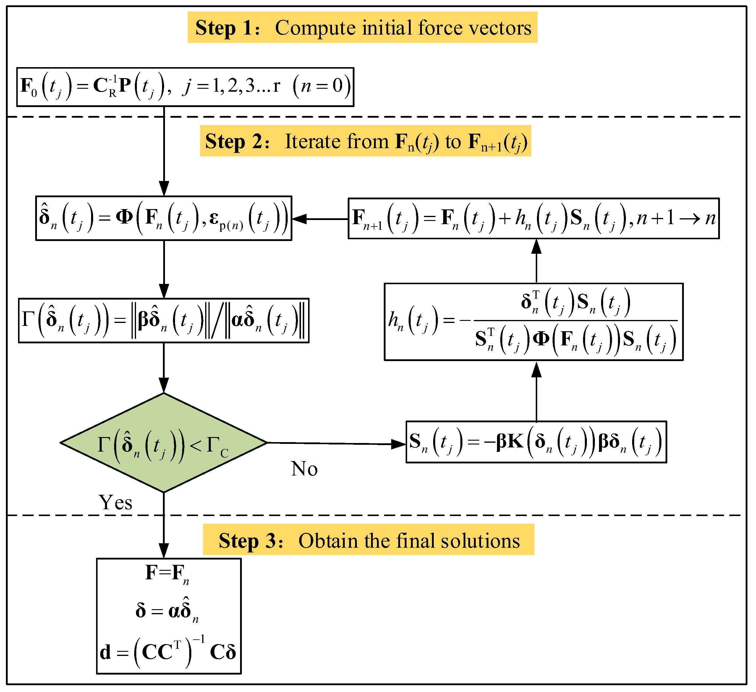
2.2. Overall Procedure of LIM

For nonlinear elastic material problems, the current strain state is uniquely determined by the current stress state and is independent of the stress history. In LIM, the loading process need not be divided and can be deemed as one large step, which is the connotation of the “large increment method”. At this incremental step, the governing equations in LIM can be established, as discussed in Section 2.1. For the statically indeterminate systems, based on the generalized inverse matrix theory, the general solutions of generalized inner forces can be obtained from the non-square equilibrium equations. Further, the generalized deformation of the system can be obtained from the constitutive equations and the special solution of generalized inner forces. The generalized inner force is searched from the general solutions and it is considered as the final result until the generalized deformation satisfies the compatibility condition. Therefore, the search process can be deemed as an optimization process. The deformation compatibility is taken as the optimization objective, and the equilibrium equations and constitutive equations are taken as the constrained conditions. Thus, the conjugate gradient method [28] is introduced for the constrained optimization problem.

However, for elastoplastic material problems, the current strain state not only depends on the current stress state but also depends on the history records of stress and strain in the constitutive equations. Here, the loading process is considered as pseudotime (t) process. To consider the loading history, the loading process needs to be divided into multiple incremental steps along the axis of time, t₀ = 0 < t₁ < t₂ <…< t_r. Thus, the corresponding external load vector can be written as P(t_j) at each incremental step, where j is the number of incremental steps. The computational procedure of LIM for elastoplastic material problems at each incremental step is the same as that for elastic material problems, except for the constitutive equations. The overall computational procedure of LIM for plastic material problems is carried out as shown in Figure 1.

• Step 1: Compute initial force vectors.

For each incremental step, the special solution of the generalized inner force vector F₀(t_j) is obtained by the equilibrium equations

$$F_0\left(t_j\right)=C_{\mathrm{R}}^{-1}P\left(t_j\right), j=1,2,3\dots r,$$

(23)

which will be taken as the initial values (n = 0).

• Step 2: Iterate from F_n(t_j) to F_n+1(t_j).

(a) Based on the F_n(t_j), the generalized deformation vector ${\widehat{\mathsf{\delta }}}_n\left(t_j\right)$ at each incremental step can be computed by the constitutive equations with the load history,

$${\widehat{\mathsf{\delta }}}_n\left(t_j\right)=\mathsf{\Phi }\left(F_n\left(t_j\right),{\mathsf{\epsilon }}_{\mathrm{p}(n)}\left(t_j\right)\right), j=1,2,\dots ,r.$$

(24)

Here, ε_p(n)(t_j) is the plastic strain at time t_j, which needs to be solved by plastic flow rule according to the plastic strain ε_p(n)(t_j−1) at time t_j and stress σ_(n)(t_j) obtained. In the calculation of this incremental step, the strain history of elastoplastic materials is incorporated.

(b) For each incremental step, the compatibility error of the system is checked by

$$\mathsf{\Gamma }\left({\widehat{\mathsf{\delta }}}_n\left(t_j\right)\right)=\frac{‖\mathsf{\beta }{\widehat{\mathsf{\delta }}}_n\left(t_j\right)‖}{‖{\widehat{\mathsf{\delta }}}_n\left(t_j\right)‖},j=1,2,\dots ,r.$$

(25)

If the compatibility error of the system at each incremental step $\mathsf{\Gamma }\left({\widehat{\mathsf{\delta }}}_n\left(t_j\right)\right)<{\mathsf{\Gamma }}_{\mathrm{C}}$ (Γ_C is the predetermined critical compatibility error and Γ_C = 10⁻⁶ is adopted in this paper), the deformation is considered to be sufficiently compatible, and the iteration is stopped and Step 3 starts. Otherwise, the generalized deformation vector is not compatible enough, and F_n(t_j) needs to be modified to improve the compatibility of the deformation vector.

(c) F_n(t_j) is improved by the conjugate gradient method. The search direction is calculated at each incremental step,

$$S_n\left(t_j\right)=-\mathsf{\beta }{K}_n\left({\mathsf{\delta }}_n\left(t_j\right)\right)\mathsf{\beta }{\mathsf{\delta }}_n\left(t_j\right),\hspace{1em}j=1,2,\dots ,r,$$

(26)

where $K_n\left({\mathsf{\delta }}_n\left(t_j\right)\right)$ is the current stiffness matrix obtained by calculating the inverse of the flexibility matrix ${\mathsf{\Phi }}_n\left(F_n\left(t_j\right)\right)$. Determine the search step length at each incremental step

$$h_n\left(t_j\right)=-\frac{{\mathsf{\delta }}_n^{\mathrm{T}}\left(t_j\right)S_n\left(t_j\right)}{S_n^{\mathrm{T}}\left(t_j\right){\mathsf{\Phi }}_n(F_n\left(t_j\right))S_n\left(t_j\right)},\hspace{1em}j=1,2,\dots ,r.$$

(27)

(d) The $F_{n+1}\left(t_j\right)$ is computed as

$$F_{n+1}\left(t_j\right)=F_n\left(t_j\right)+h_n\left(t_j\right)S_n\left(t_j\right),\hspace{1em}j=1,2,\dots ,r.$$

(28)

Replace n+1 with n and return to the start of Step 2.

• Step 3: Compute the final results.

  $$\begin{array}{c}F=F_n\\ \mathsf{\delta }=\mathsf{\alpha }{\widehat{\mathsf{\delta }}}_n\\ d={\left(C{C}^{\mathrm{T}}\right)}^{-1}\mathbf{C}\mathsf{\delta }\end{array}$$

  (29)

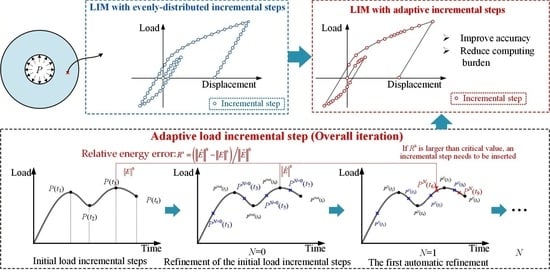
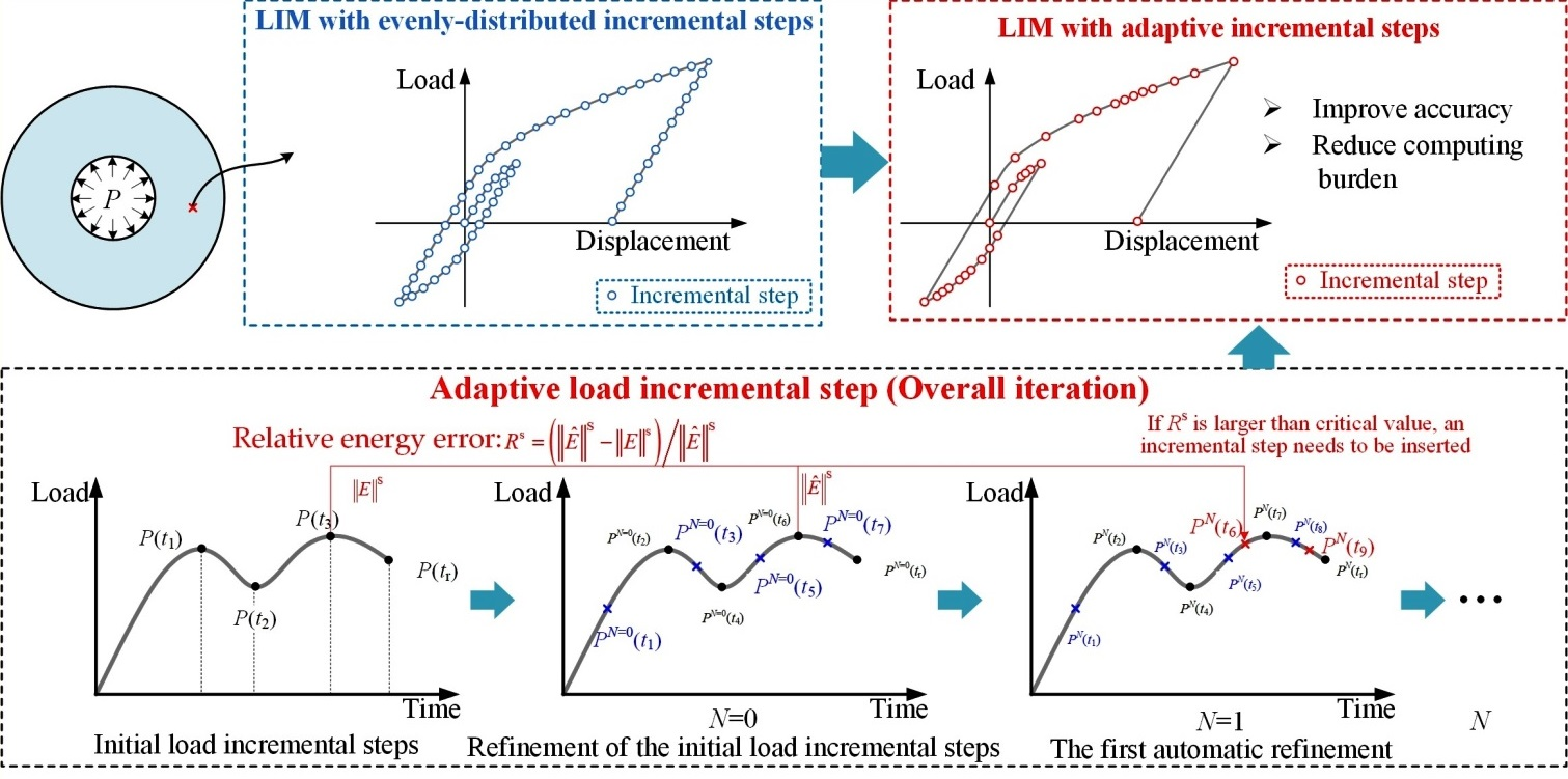
3. Adaptive Load Incremental Step Strategy in LIM

Generally, the incremental steps in LIM are chosen evenly on the loading process for simplicity [15,18,21,23,26]. In this case, more incremental steps would usually make the results more accurate but will lead to a higher number of calculations. For elastoplastic materials, the allocation of the load incremental steps has a significant effect on the final result. If the effect of load incremental step on the final results is used to automatically allocate the incremental steps, both the computational accuracy and efficiency are improved. Thus, in this section, a method to estimate the effect extent is first introduced, and then an adaptive load incremental step strategy is proposed.

3.1. Posteriori Error Estimation

To evaluate the effect extent of a certain incremental step on the final result, the posteriori error estimation of the system energy is introduced [29,30]. For simplicity, the relative energy error of the system of a certain incremental step is introduced as

$$R^{\mathrm{s}}=\frac{{‖e‖}^{\mathrm{s}}}{{‖E‖}^{\mathrm{s}}+{‖e‖}^{\mathrm{s}}}$$

(30)

where ${‖E‖}^{\mathrm{s}}$ is the total system energy at this incremental step obtained by the pre-refined loading sequence, and ${‖e‖}^{\mathrm{S}}$ is the energy error. The total energy ${‖E‖}^{\mathrm{s}}$ can be derived by

$${‖E‖}^{\mathrm{s}}={\displaystyle \sum _{i=1}^m{‖E‖}^{{\mathrm{e}}_i}},$$

(31)

where ${‖E‖}^{{\mathrm{e}}_i}$ is the energy of i-th element and m is the total element number of the system; it can be calculated by [30]

$${‖E‖}^{{\mathrm{e}}_i}=\frac{1}{2}{\displaystyle {\int }_{{\mathsf{\Omega }}^{{\mathrm{e}}_i}}{\left({\mathsf{\sigma }}^{\mathrm{e}}\right)}^{\mathrm{T}}{D}^{-1}{\mathsf{\sigma }}^{\mathrm{e}} \mathrm{d}{\mathsf{\Omega }}^{{\mathrm{e}}_i}}.$$

(32)

The energy error ${‖e‖}^{\mathrm{S}}$ is expressed as

$${‖e‖}^{\mathrm{S}}={‖\widehat{E}‖}^{\mathrm{S}}-{‖E‖}^{\mathrm{S}},$$

(33)

in which ${‖\widehat{E}‖}^{\mathrm{S}}$ is the total system energy obtained by the post-refined loading sequence. The greater the error R^s, the greater the effect extent on the final results.

3.2. Adaptive Load Incremental Step Procedure of LIM

According to the effect extent obtained by posteriori error estimation of the system energy, more incremental steps are allocated to the segment of loading process that has a greater effect on the results, by contrast, less incremental steps are allocated to the segment of loading process that has a smaller effect on the results. In this case, the calculation capacity can be allocated more reasonably to achieve higher calculation accuracy with lower calculation amount. Combined with the characteristics of LIM, an adaptive load incremental step procedure is proposed as shown in Figure 2.

• Step 1: Compute energy error for each initial incremental step.

(a) Initial group of incremental steps with a relatively large increment size are arranged evenly on the loading process as shown in Figure 2(i). The results with the initial incremental steps are calculated by LIM, as presented in Section 2.

(b) The refined group of incremental steps (N = 0) are obtained by the uniform refinement of the initial load incremental steps as shown in Figure 2(ii). Then, the results with the refined incremental steps are calculated by LIM.

(c) The energy error for each initial incremental step is calculated by Equation (30) based on the results with pre-refined and post-refined incremental steps, as described in Section 3.1.

• Step 2: Refine incremental steps.

(a) Whether there is a need to add more incremental steps is determined based on energy errors of each incremental step. If the energy error R^s at all incremental steps is less than the given critical energy error R_C, the adaptive load incremental step procedure is stopped. If the energy error on a certain incremental step R^s(t_j) is greater than the given critical energy error R_C, an incremental step is inserted before the incremental step, such as P^N(t₆) and P^N(t₉) inserted before P^N(t₇) and P^N(t_r), respectively, as shown in Figure 2(iii). Generally, the initial value of generalized inner forces of the inserted incremental steps to preform LIM are assumed as the special solutions of the generalized inner forces F₀. However, for improving the computational efficiency, the special solutions of the generalized inner forces on the inserted incremental steps are replaced by that derives from the post-refined generalized inner forces, i.e.,

$$F_0^{*}{}^{N+1}=\frac{F^N\left(t_{j-1}\right)+F^N\left(t_j\right)}{2}$$

(34)

The computational efficiency is compared between the special solutions F₀ and the derived solutions by the post-refined generalized inner forces ${\mathrm{F}}_0^{*N+1}$ in Section 4.

(b) After refining the incremental steps, the results are calculated by LIM and the energy error is computed. Replace N + 1 with the number of refinement N and return to the start of Step 2 until the refinement is not needed.

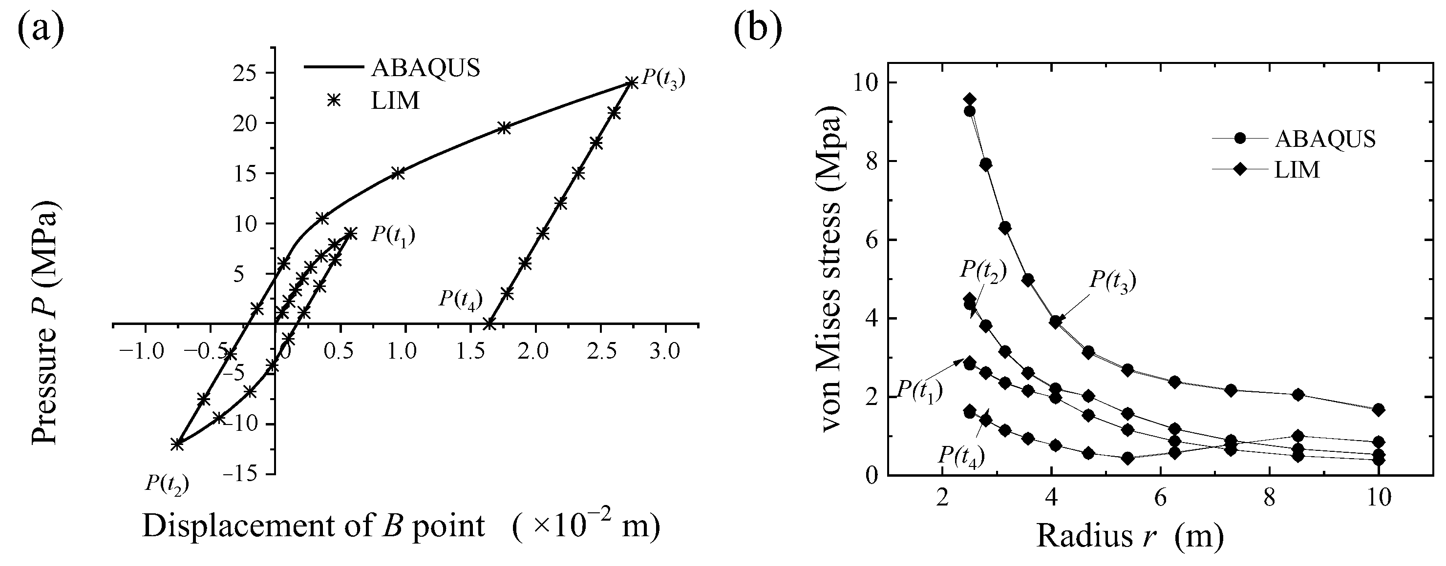
4. Numerical Example and Discussion

A numerical example is presented to verify the adaptive load incremental step of LIM in this section. A two-dimensional thick wall cylinder with bilinear hardening material model [7,20] under cyclic loading with four turning points is analyzed for taking plasticity into account [20,21], as shown in Figure 3. The material parameters are Young’s modulus E_e = 2 GPa, Poisson’s ratio ν = 0.3, tangent modulus after yield E_p = 0.5 GPa, and yield stress σ_y = 2 MPa. Because of the symmetry of the thick wall cylinder, a quarter of a thick wall cylinder is considered, as shown in Figure 3b. The structure is divided by four-node continuum plane stress element with seven generalized inner forces (CPS4S7), for which more details about the element type can be found in the work of Long and Liu [31]. Before discussing the adaptive load incremental step, it is necessary to study the validity of LIM, its convergence of load incremental steps, and the efficiency of the refined generalized inner forces.

Firstly, the results of LIM are compared with those obtained by ABAQUS’s four-node bilinear plane stress element with full integration (CPS4) to show its validity. The mesh generation and material model are the same as the LIM. The cyclic pressures are distributed to each node on the inner wall. The periodic boundary conditions are applied on the edges of the quarter of thick wall cylinder by circumferential displacement of constraining nodes. The displacement of point B is obtained directly in ABAQUS results. The evenly-distributed 2¹³ incremental steps are adopted both in LIM and ABAQUS to solve the case of the thick wall cylinder. The load-displacement diagram on point B and the von Mises stress along the radius of cylinder on four turning points of cyclic loading are shown in Figure 4a,b, respectively. The results of LIM and ABAQUS show good consistency, which indicates the validity of LIM.

Secondly, the convergence of the number of evenly-distributed incremental steps in LIM is analyzed. The stress using 2¹³ evenly-distributed incremental steps is taken as the reference stress, and the relative stress errors along the radius of the thick wall cylinder on four turning points of cyclic loading are shown in Figure 5. Combined with the numerical stress errors on the last loading point P(t₄) as shown in

Table 1. Comparisons of number of incremental steps and maximum stress error on P(t₄) between the adaptive method and evenly-distributed method.

RC	Adaptive Method			Evenly-Distributed Method
	Number of Incremental Steps r	Maximum Stress Error (%)	Computing Time (s)	Number of Incremental Steps r	Maximum Stress Error (%)	Computing Time (s)
0.03	58	1.361	150	8	4.214	12
0.02	88	1.270	296	16	2.905	54
0.01	168	0.412	516	32	2.173	127
0.009	188	0.377	566	64	1.427	322
0.008	210	0.353	610	128	0.678	902
0.007	228	0.131	650	256	0.327	4650
0.006	306	0.109	905	512	0.184	13,521

, the relative stress error is convergent with the increase of the number of incremental steps.

Thirdly, the results obtained by taking the special generalized inner forces F₀ and the refined generalized inner forces ${\mathrm{F}}_0^{*}$ as the initial value to perform LIM are compared. For simplicity, the thick wall cylinder is analyzed by applying a pressure P = 30 MPa, and the incremental steps are evenly-distributed. As shown in

Table 2. Comparison of results using different initial generalized internal forces.

Refinement Number N	Incremental Steps r	Initial Compatibility Error Γ(δ)		Number of Iterations n
		Special Solutions F0	Refined Solutions ${\mathrm{F}}_0^{*}$	Special Solutions F0	Refined Solutions ${\mathrm{F}}_0^{*}$
1	8	0.235	0.045	27	22
2	16	0.235	0.048	29	25
3	32	0.235	0.018	31	23
4	64	0.235	0.008	38	30
5	128	0.235	0.006	36	21
6	256	0.235	0.0002	37	25
7	512	0.235	0.0001	48	17
8	1024	0.235	0.00005	111	14

, as the refinement number N increases, the initial compatibility error Γ(δ) obtained by the refined generalized inner forces ${\mathrm{F}}_0^{*}$ decreases, whereas the Γ(δ) obtained by the special generalized inner forces remains constant. In addition, the number of iterations n in LIM using the special generalized inner forces increases with the incremental step number, however, the number of iterations n using the refined generalized inner forces is approximately invariant, or even reduced. The results indicate that the efficiency using refined generalized inner forces ${\mathrm{F}}_0^{*}$ as the initial generalized inner forces is higher.

Lastly, but most importantly, the validity, efficiency, and characteristics of the adaptive load incremental strategy in LIM are studied in the following. The number and size of the incremental steps are adjusted automatically according to the relative energy error R_C. The number of incremental steps and maximum stress error at the last step P(t₄) with different critical relative energy error R_C are shown in Table 1. With the decrease in critical relative energy errors R_C, the number of incremental steps increases, and the maximum stress error on P(t₄) decreases. The comparison of computing cost of the adaptive method and the evenly-distributed method are shown in Table 1, and the procedures of adaptive load increment method in LIM are realized by MATLAB code. With the decrease in the maximum stress error on P(t₄), the computing time increases for both adaptive method and evenly-distributed method. However, the adaptive method can obtain higher accuracy with lower computing time compared with the evenly-distributed method. The computational efficiency is sharply improved by the adaptive method.

In addition, the relative stress errors along the radius of the thick wall cylinder on four turning points of cyclic loading with different critical relative energy error R_C are shown in Figure 6. The relative stress errors decrease with the decrease in the critical relative energy error.

The location distribution of the adaptive load incremental steps is shown in Figure 7. It is found that more incremental steps are distributed in the plastic segments of the material. This means that the plastic section of the material has a greater effect on the final result.

Different element types are considered to further confirm efficiency of the proposed adaptive method. The thick wall cylinder is divided by a four-node continuum plane stress element with five generalized inner forces (CPS4S5) [31]. A monotonic pressure loading path is loaded in the inner wall. This method still improves the computation efficiency sharply. More details can be found in Appendix A.

5. Discussion and Conclusions

This paper proposes and implements an adaptive load incremental step strategy in the framework of LIM for elastoplastic material problems. By introducing the posteriori error estimation of energy, the automatic refinement procedure for the load incremental steps is established. The initial value of refined incremental steps to perform LIM are derived from the final results obtained by the pre-refined incremental steps to improve the efficiency. The efficiency and characteristics of the adaptive load incremental step in LIM are verified by the bilinear material problems under cyclic loading. The strategy improves the accuracy of results and computational efficiency by allocating the incremental steps rationally. Additionally, the accuracy of the result can be quantitatively evaluated.

For adaptive increment step in LIM, some large increment steps are initially given, and then the additional increment steps will be inserted according to the impact degree of each step on results. For the adaptive increment step in the traditional displacement method, an increment step is initially given, and then the size of next step will be adjusted according to the convergence and convergence speed. Thus, the two adaptive increment step methods used in LIM and traditional displacement method are completely different strategies.

Compared with the adaptive load incremental step of displacement-based FEM, LIM exhibits two major advantages for elastoplastic material problems. (1) LIM can significantly reduce the calculation burden, especially for the cases of a large number of elements. In LIM, the governing equations are separated into two categories, the global equilibrium and compatibility equations and the local constitutive equations. Thus, the establishment of the global equilibrium equations and the calculation of the inverse of the equilibrium matrix only need one time for all of the procedures in the case of small deformations, which can significantly reduce the calculation burden. (2) The error accumulation in the displacement-based FEM is well restrained, owning to the replacement of the step-by step procedure at the global stage by the refine procedure in LIM. In addition, the two categories of governing equations endow LIM with greater advantages in parallel computation with the adaptive load incremental steps.

There are essential differences between LIM and the displacement finite element method in terms of initial unknown variables and calculation processes. Based on the features of LIM, the following points should be considered when exploring future potential, (1) the exploration of LIM basic theory, such as the development of standard element library and material library, (2) geometrically nonlinear analysis, and (3) the stochastic finite element.

References

1. Molina, A.; Curiel-Sosa, J.L. A multiscale finite element technique for nonlinear multi-phase materials. Finite Elem. Anal. Des. 2015, 94, 64–80. [Google Scholar] [CrossRef] [Green Version]
2. Zienkiewicz; Taylor, R.C. The Finite Element Method; McGraw Hill: New York, NY, USA, 1989. [Google Scholar]
3. Arkov, D.P.; Kochetkova, O.V.; Gureeva, N.A.; Matveyev, A.S.; Shiryaeva, E.V. Simulation of the stress-strain state of shells under internal pressure using the mixed finite element method, taking into account physical nonlinearity. IOP Conf. Ser. Mater. Sci. Eng. 2020, 873, 012032. [Google Scholar] [CrossRef]
4. Du, X.; Dang, S.; Yang, Y.; Chai, Y. The Finite Element Method with High-Order Enrichment Functions for Elastodynamic Analysis. Mathematics 2022, 10, 4595. [Google Scholar] [CrossRef]
5. Xu, Y.; Li, H.; Chen, L.; Zhao, J.; Zhang, X. Monte Carlo Based Isogeometric Stochastic Finite Element Method for Uncertainty Quantization in Vibration Analysis of Piezoelectric Materials. Mathematics 2022, 10, 1840. [Google Scholar] [CrossRef]
6. Simo, J.C.; Hughes, T.J.R. Computational Inelasticity; Springer: Berlin/Heidelberg, Germany, 1997. [Google Scholar]
7. Chen, H. Elasticity and Plasticity; China Architecture & Building: Beijing, China, 2005. [Google Scholar]
8. Cook, R.D.; Malkus, D.S.; Plesha, M.E. Concepts and Applications of Finite Element Analysis; Wiley: Hoboken, NJ, USA, 1989. [Google Scholar]
9. Tracey, D.M.; Freese, C.E. Adaptive load incrementation in elastic-plastic finite element analysis. Comput. Struct. 1981, 13, 45–53. [Google Scholar] [CrossRef]
10. Abbo, A.J.; Sloan, S. An automatic load stepping algorithm with error control. Int. J. Numer. Methods Eng. 1996, 39, 1737–1759. [Google Scholar] [CrossRef]
11. Fernandes, M.; Cardoso, C.O.; Mansur, W.J. An adaptive load stepping algorithm for path-dependent problems based on estimated convergence rates. Comput. Model. Eng. Sci. 2017, 113, 325–342. [Google Scholar]
12. Zahavi, E. The Finite Element Method in Machine Design; Prentice Hall: Hoboken, NJ, USA, 1992. [Google Scholar]
13. Bathe, K.J. Finite Element Procedures; Klaus-Jurgen Bathe: Cambridge, MA, USA, 2006. [Google Scholar]
14. Kaljevi, I.; Patnaik, S.N.; Hopkins, D.A. Development of finite elements for two-dimensional structural analysis using the integrated force method. Comput. Struct. 1996, 59, 691–706. [Google Scholar] [CrossRef] [Green Version]
15. Zhang, C.; Liu, X. A large increment method for material nonlinearity problems. Adv. Struct. Eng. 1997, 1, 99–110. [Google Scholar] [CrossRef]
16. Neuenhofer, A.; Filippou, F.C. Geometrically nonlinear flexibility-based frame finite element. J. Struct. Eng. 1998, 124, 704–711. [Google Scholar] [CrossRef]
17. Santos, H. Variationally consistent force-based finite element method for the geometrically non-linear analysis of Euler–Bernoulli framed structures. Finite Elem. Anal. Des. 2012, 53, 24–36. [Google Scholar] [CrossRef]
18. Barham, W.; Aref, A.J.; Dargush, G.F. Development of the large increment method for elastic perfectly plastic analysis of plane frame structures under monotonic loading. Int. J. Solids Struct. 2005, 42, 6586–6609. [Google Scholar] [CrossRef] [Green Version]
19. Barham, W.S.; Aref, A.J.; Dargush, G.F. Flexibility-based large increment method for analysis of elastic–perfectly plastic beam structures. Comput. Struct. 2005, 83, 2453–2462. [Google Scholar] [CrossRef]
20. Barham, W.; Aref, A.; Dargush, G. On the elastoplastic cyclic analysis of plane beam structures using a flexibility-based finite element approach. Int. J. Solids Struct. 2008, 45, 5688–5704. [Google Scholar] [CrossRef] [Green Version]
21. Barham, W.S.; Idris, A.A. Flexibility-based large increment method for nonlinear analysis of Timoshenko beam structures controlled by a bilinear material model. Structures 2021, 30, 678–691. [Google Scholar] [CrossRef]
22. Aref, A.J.; Guo, Z.Y. Framework for finite-element-based large increment method for nonlinear structural problems. J. Eng. Mech. -Asce 2001, 127, 739–746. [Google Scholar] [CrossRef]
23. Jia, H.-x. Large increment method for elastic and elastoplastic analysis of plates. Finite Elem. Anal. Des. 2014, 88, 16–24. [Google Scholar] [CrossRef]
24. JIa, X.; Long, D.; Liu, X. Development of the Large Increment Method in Analysis for Thin and Moderately Thick Plates. J. Shanghai Jiaotong Univ. 2014, 19, 265–273. [Google Scholar] [CrossRef]
25. JIa, X.; Liu, X. Force-Based Quadrilateral Plate Bending Element for Plate Using Large Increment Method. J. Donghua Univ. 2015, 32, 345–350. [Google Scholar] [CrossRef]
26. Bordas; Alain, S.P. An element nodal force-based large increment method for elastoplacisity. AIP Conf. Proc. 2010, 1233, 1401–1405. [Google Scholar]
27. Ben-Israel, A.; Greville, T. Generalized Inverse: Theory and Application; Springer Science & Business Media: Berlin/Heidelberg, Germany, 1974. [Google Scholar]
28. Press, W.H.; Flannery, B.P.; Teukolsky, S.A.; Vetterling, W.T. Numerical Recipes in C: The Art of Scientific Computing; University Press: Cambridge, UK, 1989. [Google Scholar]
29. Zienkiewicz, O.C.; Zhu, J.Z. A simple error estimator and adaptive procedure for practical engineerng analysis. Int. J. Numer. Methods Eng. 1987, 24, 337–357. [Google Scholar] [CrossRef]
30. Guo, Z.Y.; Zhao, Y.J.; Chen, Z.H.; Liao, M.M.; Li, Z.L.; Liu, B. A Mesh Adaptive Procedure for Large Increment Method. Int. J. Appl. Mech. 2015, 7, 1550061. [Google Scholar] [CrossRef]
31. Long, D.; Liu, X. Development of 2D Hybrid Equilibrium Elements in Large Increment Method. J. Shanghai Jiaotong Univ. 2013, 18, 205–215. [Google Scholar] [CrossRef]
Figure 1. Computational procedure of LIM for elastoplastic problems.
Mathematics 11 00524 g001
Figure 2. Adaptive load incremental step procedure of LIM.
Mathematics 11 00524 g002
Figure 3. Thick wall cylinder problem: (a) thick wall cylinder subjected to internal load, (b) the finite element mesh and symmetrical boundary condition, (c) stress-strain diagram for bilinear material model, and (d) cyclic pressure loading path.
Mathematics 11 00524 g003
Figure 4. Comparison of LIM and ABAQUS: (a) load-displacement diagram and (b) von Mises stress along radius.
Mathematics 11 00524 g004
Figure 5. Convergence analysis of the number of incremental steps on four turning points of cyclic loading: (a) P (t1), (b) P (t2), (c) P (t3), and (d) P (t4).
Mathematics 11 00524 g005
Figure 6. The relative stress errors along the radius of the thick wall cylinder on four turning points of cyclic loading with different critical relative energy error RC: (a) P (t1), (b) P (t2), (c) P (t3), and (d) P (t4).
Mathematics 11 00524 g006
Figure 7. Location distribution of the adaptive load incremental steps in LIM. (RC = 0.01).
Mathematics 11 00524 g007