Demand Forecasting of Spare Parts Using Artificial Intelligence: A Case Study of K-X Tanks

Abstract

The proportion of the inventory range associated with spare parts is often considered in the industrial context. Therefore, even minor improvements in forecasting the demand for spare parts can lead to substantial cost savings. Despite notable research efforts, demand forecasting remains challenging, especially in areas with irregular demand patterns, such as military logistics. Thus, an advanced model for accurately forecasting this demand was developed in this study. The K-X tank is one of the Republic of Korea Army’s third generation main battle tanks. Data about the spare part consumption of 1,053,422 transactional data points stored in a military logistics management system were obtained. Demand forecasting classification models were developed to exploit machine learning, stacked generalization, and time series as baseline methods. Additionally, various stacked generalizations were established in spare part demand forecasting. The results demonstrated that a suitable selection of methods could help enhance the performance of the forecasting models in this domain.

1. Introduction

Demand forecasting is widely performed in various fields, such as electric power, finance, and service. Forecast models associated with spare part consumption are significant, especially in the equipment management and sustainment industry [1]. In general, the cost of spare parts occupies a considerable proportion of the equipment maintenance cost [2]. Demand forecasting for spare parts in the military is an essential factor in equipment utilization. High demand forecasting accuracy for spare parts can improve equipment utilization and cost efficiency [3]. Therefore, big-data-based methods to forecast the demand for spare parts have received considerable attention in the fourth industrial revolution [4]. Securing adequate spare parts is crucial for ensuring the uninterrupted operation of different types of equipment, reducing budgets, and efficiently managing the munitions field. Thus, considerable research has been conducted to forecast the demand for spare parts [5]. Many countries pursue an increased operating rate of new and existing weapon systems to ensure national security and reasonable defense budgeting. Thus, in the event of equipment failure, timely and prompt acquisition and replacement of spare parts are required [6]. It is necessary to forecast the demand for consumable spare parts at least one year before their total consumption. Through such forecasting frameworks, a country can obtain the necessary amounts of spare parts for year X in the year X-1. Therefore, the forecasting accuracy for the demand for spare parts is a critical factor in ensuring the equipment’s operating rate, reducing the procurement and maintenance periods, and enhancing budget efficiency [3].

Notably, as modern weapon systems become more technologically and cost-intensive, the asset value of the equipment and the budget for repairing accessories are continuously increasing. Generally, the demand for spare parts differs according to the type of equipment and is intermittent and irregular. Moreover, the lifetime of spare parts introduced for equipment is often more significant than that of the equipment [7]. These aspects can increase the maintenance cost of modern weapon systems. Therefore, a scientific and accurate demand forecasting model must be developed to optimize equipment utilization and inventory costs. Consequently, the accuracy of the demand forecasting models for spare parts must be increased [8]. Many researchers have attempted to increase demand forecasting accuracy for spare parts. The most commonly used technique is the time series. Three to eight technologies, such as the moving average method and the exponential smoothing method, can be combined to increase efficiency.

In contrast to the existing time series techniques, this study applied artificial intelligence (AI) techniques to enhance the forecasting accuracy of the demand for spare parts for the K-X tank, which is the first domestic and core third generation tank since the Republic of Korea Army was built. Consequently, the accuracy was improved by applying several models and previous time series techniques [9]. Currently, AI is a key technology of the fourth industrial revolution. Therefore, this study adopted meta-learning techniques recently applied to big data. Time series techniques, data mining, and attention recurrent neural networks (RNNs) were used based on a meta-learning algorithm. The key objectives of the study can be summarized as follows:

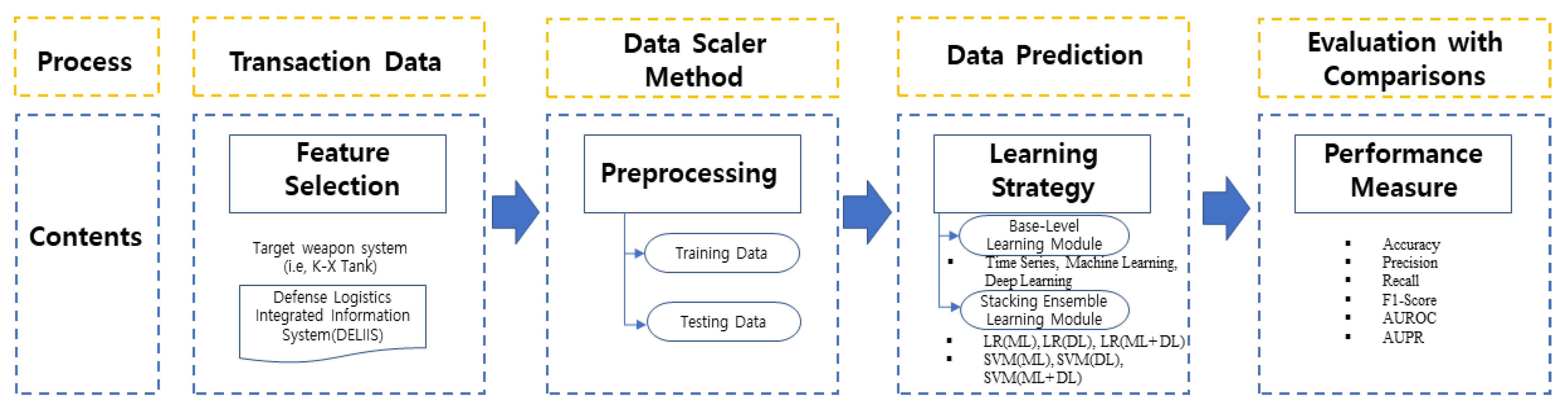
• To investigate various spare part demand forecasting models associated with classification methods, more specifically time series analysis, data mining, and deep learning, based on stacking and pairing spare parts and demand datasets.
• To identify the model with the highest forecasting accuracy based on statistical analyses.
• To highlight future research directions to ensure better management and spare part demand forecasting in the defense and logistics sectors.

The rest of the paper is organized as follows. Section 2 reviews the existing studies on time series, machine learning, and stacked generalization. The proposed model, data extraction techniques, and variables are elaborated on in Section 3. Section 4 presents a comparative analysis of the results of each technique. Finally, the concluding remarks and highlights are presented in Section 5.

2. Literature Review

2.1. Time Series

Time series analyses are widely employed in many demand forecasting domains and represent representative quantitative techniques to forecast changes from historical patterns [10]. A few researchers used first- and second-order exponential smoothing methods to estimate the number of traffic-accident-related injuries and fatalities in Jordan from 1981 to 2016. The results were compared to those obtained using methods based on the mean absolute percentage error, mean absolute deviation, and mean squared deviation. The second-order exponential smoothing method exhibited excellent performance [11]. Our demand forecast model for repair units involved 5–8 time series techniques for each military domain, with 3 techniques used for the Army. Models used by most South Korean troops involve 5–9 time series techniques. In this methodology, the actual demands for year X after implementing the year X-1 demand forecast are compared, and a relatively simple demand forecasting technique is compared to the private technique [5,6].

2.2. Machine Learning

In this study, we applied data mining and deep learning methodologies. Data mining involves generating knowledge by investigating, analyzing, and modeling useful information and relations from big data [12]. Data mining methods include decision trees (DTs), Bayesian networks, and support vector machines (SVM). In the DT-based approach, information is analyzed based on decision-making rules to sort the information into tree structures, classify the concerned class into many classes, or make predictions [13].

Deep learning involves deep neural networks consisting of links. Such networks imitate human neural networks and are composed of numerous layers [14,15]. A multi-layer perceptron (MLP) is an orthodromic artificial neural network in which single-layer perceptron networks are connected in multiple layers. An MLP can overcome the disadvantage of single-layer perceptron systems that cannot manage data that cannot be linearly separated [16,17]. Moreover, to enhance MLP approaches, RNNs that involve a circulation structure have been developed. In such frameworks, the information of a specific instance is stored in each memory block and transmitted according to the following schedule. RNNs perform excellently in processing sequential data, such as text, voice, and time series data [18]. Using the long short-term memory (LSTM) algorithm, RNNs can eliminate the problem of long-term dependency, and such frameworks have thus been applied in various fields [19]. Gated recurrent units (GRU) represent the modified model of LSTM; such models do not involve the issue of gradient vanishing and involve a less complex calculation process [20].

A convolutional neural network (CNN) is one of the techniques that corrects problems that occur when processing data such as images or videos in a deep neural network [21]. Previous studies applied CNNs to solve the urban functions and socioeconomic status with short-term travel demand forecast patterns. The methodology that improved the accuracy of travel demand prediction by combining deep learning architecture with a traditional CNN was applied to this study [22].

2.3. Stacked Generalization

Stacked generalization is a learning method based on one-shot learning. In this framework, a model performs rapid learning when one-shot data are provided using the rich factor data instead of the classification analysis method [23]. Related techniques include the bagging technique, which can reduce the variance, and the AdaBoosting technique, which minimizes the bias [24]. Stacked generalization aims to assemble different models, thereby reinforcing the strengths of each model and supplementing their weaknesses in establishing a highly accurate model. The commonly used models include SVM, DT, and random forests [25]. Stacked generalization, also known as meta-learning, estimates the generalized error of the training dataset by using several classification algorithms to reduce these errors and forecast the final test dataset [26]. In particular, stacked generalization involves two steps. In the first step, the forecasts are obtained by training various classification algorithms (Level-0 models). In the second step, these forecasts are gathered to form a meta-training set, and forecasts are obtained using the final classification algorithm (Level-1 model). Generally, higher performance can be achieved by learning the values predicted using Level-0 models and classifying them using Level-1 models than by using only Level-0 models [27].

Existing studies have highlighted that AI technology is significant in the fourth industrial revolution, as it can support future-oriented decision-making and big data. However, the South Korean military still depends on the time series technique, in which only past demand data is used. Previously, data other than demand data could not be considered. However, since establishing an information system in 2009, additional information can be accumulated, and the variables can be further examined. Moreover, machine learning techniques can enhance demand forecast accuracy in various fields. This study establishes a meta-learning technique combining RNNs and a machine learning classification approach considering time series.

3. Problem Description and Methodology

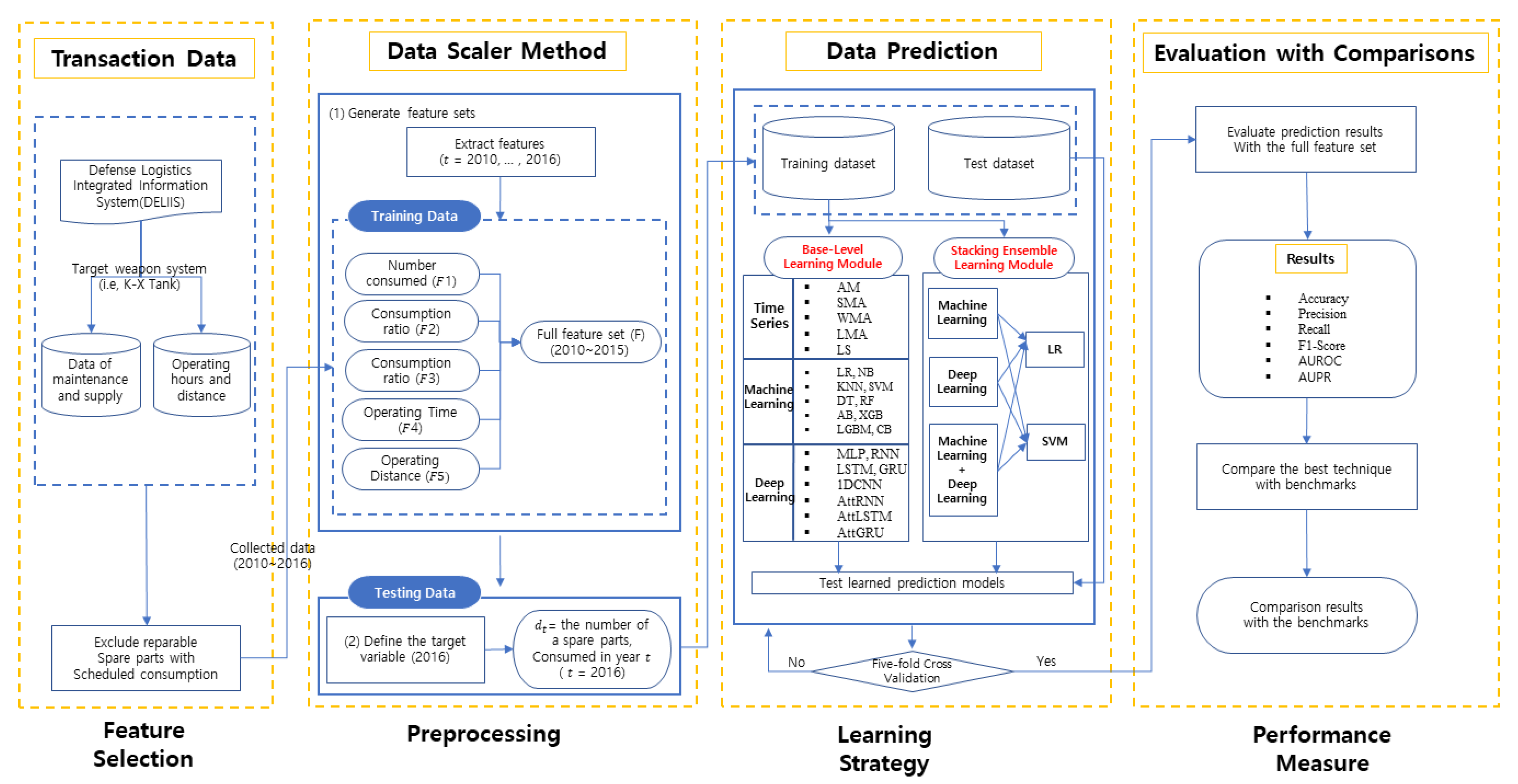
3.1. Data Collection

Since 2009, the Republic of Korea Army has been building an information system for the supply and maintenance of spare parts by using the latest information technologies and focusing on the main equipment of weapon systems. The integrated information support system, Defense Logistics Integrated Information System, is used by maintenance-related departments from the organization units of the Army, Navy, and Air Force from the Ministry of Defense. The system includes 1,053,422 transactional data points, derived from the maintenance table of the device maintenance information system of the Air Force, involving 22 variables, including maintenance data, the number of repair accessories consumed on the repair day, and component count per vehicle. The data for the target airplanes of this study were reorganized based on item type, and 10,714 spare parts were considered. In addition, variables associated with the data for yearly consumption were extracted. The target variable to be predicted corresponded to the data associated with the requirement for each item in 2017, consisting of 10,714 items. To balance the distribution of the target variable in terms of item requirement, the items included 5357 needed items and 5357 unneeded items. The 35 variables in the data corresponded to the units consumed, units procured, consumption ratios, operating times, and operating distances for seven years (2010–2016), as shown in

Table 1. Feature description.

Variable (Number of the Unit)	Meaning	Type of Variable
Number consumed (6)	Sum of spare parts consumed per item by year	Independent Variable (2010–2015)
Number procured (6)	Sum of spare parts procured per item by year
Consumption ratio (6)	Consumption ratio of spare parts consumed per item by year (Consumption ratio = number consumed/number procured)
Equipment operation time (6)	Operating time of equipment by year
Equipment operation distance (6)	Equipment operating distance by year
Number consumed (1)	Demand forecasting of spare parts consumed per item in 2016 (Binary; 0, 1)	Dependent Variable (2016)

. These variables were not independent because of the time series tendency. In particular, classification problems with time series characteristics differ from typical classification problems because the variables are specified in a specific order. We used deep learning and meta-learning, which are excellent methods for processing sequentially occurring data, to solve this problem.

3.2. Proposed Stacking Ensemble Learning System

The proposed stacking ensemble learning system consisted of a base-level learning module and a stacking ensemble learning module. The base-level learning module determined the probability of the predicted result to prepare a meta-dataset. Five-fold cross-validation was performed to prevent over-fitting when constructing a meta-dataset. See Figure 1, which represents the overview of the process.

Base-Level Learning Module. The base-level learning module can be divided into machine learning methods that do not consider time series and deep learning methods that consider time series. The machine learning methods include traditional statistical models, such as logistic regression (LR) and naive Bayes (NB), and a distance-based model, k-nearest neighbor (KNN). It also included a model that finds the hyperplane with the most significant margin between classes, the SVM model, and the tree-based bagging or boosting models, such as DTs, RFs, AdaBoost (AB), XGBoost (XGB), LightGBM (LGBM), and CatBoost (CB). Additionally, we considered the characteristics of 11 models, including the MLP.

An RNN algorithm was used as a deep learning technique to reflect the time series tendency. In particular, RNNs, GRUs, and LSTM, commonly used RNN algorithms, and AttRNN, attention GRU (AttGRU), and attention LSTM (AttLSTM) were applied with the attention mechanism to focus on features related to the target. Moreover, a 1D convolutional neural network (1DCNN) that extracts features through the convolution operation was used, leading to seven deep learning algorithms.

Stacking Ensemble Learning Module. The meta-dataset created through the learning of the base-level learning module included numerical data that expressed prediction values as probabilities. In the stacking ensemble learning module, a relatively simple linear model is usually used to combine the results predicted by the base-level learning module and the confidence [17]. Therefore, LR and SVM were used as machine learning techniques to train the meta-dataset in this study’s stacking ensemble learning module. See Figure 2 for more details on the stacking ensemble learning module. The result was computed by training the meta-dataset using the stacking ensemble learning module.

4. Experimental Study

4.1. Experimental Design

The data used in this study exhibited a time series characteristic. To reflect this time series tendency, training data were obtained by splitting the data into years to enhance the robustness of the learned model. Given that the objective was to forecast the repair accessory demand in 2017, data from 2010 to 2015 were used as input variables and trained to forecast the demand for spare parts in 2016. Subsequently, the final performance was evaluated by forecasting the demand for spare parts in 2017 using 2011 to 2016 as input variables.

Performance Indicators. The accuracy, precision, recall, and F1-score, typically used in classification problems, were used as evaluation indicators. In addition, we examined the area under the receiver operating characteristic curve (AUROC) and the area under the precision–recall curve (AUPR), which can illustrate the robustness of the model. AUROC is a real number between 0.5 and 1, and if it is closer to 1, it is better than the model. The x-axis of AUPR becomes a recall, and the y-axis becomes precision. The AUPR below it becomes the area. The Equations for each evaluation indicator are as follows:

Actual: Yes, Predicted: Yes = TP (True Positive),

Actual: Yes, Predicted: No = FP (False Positive),

Actual: No, Predicted: Yes = FN (False Negative),

Actual: No, Predicted: No = TN (True Negative)

Accuracy rate = (TP + TN)/(TP + FP + FN + TN)

Recall = TP/(TP + FN), Precision = TP/(TP + FP),

Specificity = TN/(TN + FP), F1-Score = 2 × Recall × Precision/(Recall + Precision)

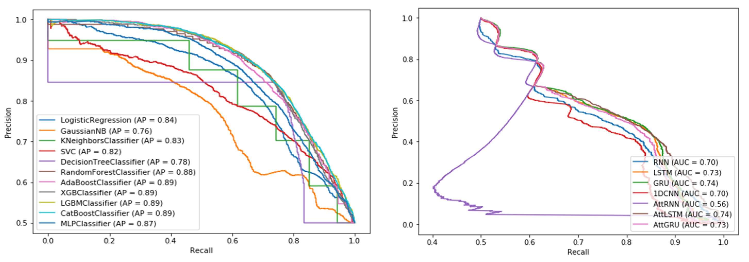
4.2. Classification Results of the Base Model

The base model consisted of time series, machine learning, and deep learning techniques. The goal of this research was to suggest a model that predicts the demand for an entire year, based on previous data for spare parts, for six years. Since lag data based on spare parts is used for verification and evaluation, cross-validation was performed by randomly classifying five folds. For the fairness of the experiment, the spare parts to be evaluated over time were always selected from the same group. The methodology of the base model transformed the state of the spare parts into representations of binary integers [0, 1] according to the occurrence of the item.

As indicated in

Table 2. Performance values of base models.

Model	Method	Accuracy	Precision	Recall	F1-Score	AUROC	AUPR	ET (Sec)
AM	Time series	0.692	0.776	0.692	0.706	0.690	0.620	0.002
SMA		0.725	0.771	0.725	0.731	0.720	0.650	0.001
WMA		0.548	0.914	0.548	0.649	0.550	0.520	0.001
LMA		0.575	0.790	0.575	0.626	0.610	0.560	0.002
LS		0.540	0.860	0.540	0.627	0.540	0.520	0.003
LR	Machine learning	0.743	0.886	0.556	0.684	0.820	0.840	0.884
NB		0.593	0.914	0.206	0.336	0.740	0.760	0.908
KNN		0.771	0.786	0.744	0.765	0.840	0.830	1.100
SVM		0.716	0.811	0.564	0.665	0.810	0.820	2.490
DT		0.801	0.838	0.747	0.79	0.790	0.780	2.521
RF		0.800	0.834	0.75	0.79	0.860	0.880	2.908
AB		0.791	0.839	0.721	0.775	0.860	0.890	3.139
XGB		0.801	0.857	0.722	0.784	0.860	0.890	4.344
LGBM		0.802	0.858	0.723	0.785	0.870	0.890	4.600
CB		0.801	0.853	0.727	0.785	0.870	0.890	9.811
MLP	Deep learning	0.775	0.829	0.692	0.754	0.840	0.870	12.407
RNN		0.646	0.614	0.787	0.69	0.700	0.700	7.902
LSTM		0.646	0.614	0.787	0.69	0.730	0.730	8.928
GRU		0.646	0.614	0.787	0.69	0.740	0.740	7.916
1DCNN		0.621	0.609	0.673	0.64	0.700	0.700	5.261
AttRNN		0.616	0.607	0.662	0.633	0.560	0.560	2.026
AttLSTM		0.646	0.614	0.787	0.69	0.740	0.740	4.576
AttGRU		0.646	0.614	0.787	0.69	0.730	0.730	4.295

, the machine learning-based model outperformed the traditional univariate time series model. In particular, the tree-based model exhibited excellent overall performance in terms of the accuracy and the F1-score. Figure 3 and Figure 4 show that the AUROC and AUPR scores were also significantly high. The deep learning-based model exhibited a high recall value. Execution time (ET) is the time required relative to the number of operations required to perform operations based on input values and algorithm changes. Given the ETs from the results, the suggested methodology can be applied in real time.

4.3. Classification Results Obtained Using the Stacking Ensemble Model

Three models were established for the stacking ensemble model, based solely on the machine learning algorithm (ML), solely on the deep learning algorithm (DL), and on a combination of ML and DL (ML + DL). Overall, the stacking ensemble model outperformed the base model in terms of the accuracy and the F1-score, as indicated in

Table 3. Performance values of the stacking ensemble models.

Model	Accuracy	Precision	Recall	F1-Score	AUROC	AUPR	ET (Sec)
LR (ML)	0.805	0.850	0.742	0.792	0.880	0.900	0.022
LR (DL)	0.647	0.614	0.789	0.691	0.750	0.730	1.060
LR (ML + DL)	0.805	0.849	0.742	0.792	0.880	0.900	1.109
SVM (ML)	0.804	0.868	0.716	0.785	0.840	0.830	0.690
SVM (DL)	0.647	0.615	0.790	0.691	0.750	0.760	3.161
SVM (ML + DL)	0.804	0.872	0.713	0.784	0.840	0.830	1.622

. Moreover, Figure 5 shows that the AUROC and AUPR scores were enhanced for the stacking model. Among the proposed stacking ensemble models, the LR (ML) and LR (ML + DL) models, both of which exhibited the highest performance, achieved an accuracy of 80.5% and an F1-score of 79.2%.

The LR fared better in the stacking ensemble learning module than the SVM in terms of recall and the F1-score, despite the SVM’s superior accuracy and precision. The precision and recall values were slightly superior to SVM (ML + DL) and SVM (DL) when the time series deep learning model was used. The deep learning-based stacking ensemble model gave a high recall, identical to the base model. Utilizing a suitable stacking ensemble learning module while considering the necessary evaluation indicators is essential in this context.

5. Conclusions

Time series, machine learning, deep learning, and stacked generalization techniques were applied to forecast the demand for spare parts. The stacked generalization techniques outperformed the existing time series method.

A significant portion of the munitions inventory is spare parts, accounting for a high percentage of the inventory. Therefore, a small improvement in forecasting for spare parts can ensure significant cost savings and higher wartime preparedness. For models with high accuracy, data expansion is required by considering intermittent demand forecasting and applying the M4 (day, month, quarter, half, year) competition methodology. Until now, only structured data were considered, but unstructured data will also be considered to increase the accuracy of future demand forecasts.

References

1. Adams, J.L.; Abell, J.B.; Isaacson, K.E. Modeling and Forecasting the Demand for Aircraft Recoverable Spare Parts; No. RAND/R-4211-AF/OSD; Rand Corp.: Santa Monica, CA, USA, 1993. [Google Scholar]
2. Fisher, M.; Hammond, J.; Obermeyer, W.; Raman, A. Configuring a supply chain to reduce the cost of demand uncertainty. Prod. Oper. Manag. 1997, 6, 211–225. [Google Scholar] [CrossRef]
3. Kim, J. Text mining-based approach for forecasting spare parts demand of K-X tanks. In Proceedings of the 2018 IEEE International Conference on Industrial Engineering and Engineering Management (IEEM), Bangkok, Thailand, 16–19 December 2018; pp. 1652–1656. [Google Scholar]
4. Bousdekis, A.; Apostolou, D.; Mentzas, G. Predictive maintenance in the 4th industrial revolution: Benefits, business opportunities, and managerial implications. IEEE Eng. Manag. Rev. 2019, 48, 57–62. [Google Scholar] [CrossRef]
5. Regatteri, A.; Gamberi, M.; Gamberini, R.; Manzini, R. Managing lumpy demand for aircraft spare parts. J. Air Transp. Manag. 2005, 11, 426–431. [Google Scholar] [CrossRef]
6. Kim, J.; Lee, H.; Choi, S. Machine learning based approach for demand forecasting anti-aircraft missiles. In Proceedings of the 2018 5th IEEE International Conference on Industrial Engineering and Applications (ICIEA), Singapore, 26–28 April 2018; pp. 367–372. [Google Scholar]
7. Sánchez, A.; Sunmola, F. Factors influencing effectiveness of lean maintenance repair and overhaul in aviation. In Proceedings of the International Symposium on Industrial Engineering and Operations Management, Rabat, Morocco, 11–13 April 2017; pp. 855–863. [Google Scholar]
8. Brown, B.B. Characteristics of Demand for Aircraft Spare Parts; Rand Corporation: Santa Monica, CA, USA, 1956. [Google Scholar]
9. Ulrich, M.; Jahnke, H.; Langrock, R.; Pesch, R.; Senge, R. Classification-based model selection in retail demand forecasting. Int. J. Forecast. 2022, 38, 209–223. [Google Scholar] [CrossRef]
10. Chatfield, C. Time-Series Forecasting; Chapman and Hall/CRC: London, UK, 2000. [Google Scholar]
11. Rahamneh, A. Using single and double exponential smoothing for estimating the number of injuries and fatalities resulted from traffic accidents in Jordan (1981–2016). Middle-East J. Sci. Res. 2017, 25, 1544–1552. [Google Scholar]
12. Hand, D.J. Principles of data mining. Drug Saf. 2007, 30, 621–622. [Google Scholar] [CrossRef] [PubMed]
13. Kass, G.V. An exploratory technique for investigating large quantities of categorical data. Appl. Stat. 1980, 29, 119–127. [Google Scholar] [CrossRef] [Green Version]
14. Bengio, Y.; Courville, A.; Vincent, P. Representation learning: A review and new perspectives. IEEE Trans. Pattern Anal. Mach. Intell. 2013, 35, 1798–1828. [Google Scholar] [CrossRef] [PubMed] [Green Version]
15. Schmidhuber, J. Deep learning in neural networks: An overview. Neural Netw. 2014, 61, 85–117. [Google Scholar]
16. Werbos, P.J. Backpropagation through time: What it does and how to do it. Proc. IEEE 1990, 78, 1550–1560. [Google Scholar] [CrossRef] [Green Version]
17. Kumpati, S.N.; Kannan, P. Identification and control of dynamical systems using neural networks. IEEE Trans. Neural Netw. 1990, 1, 4–27. [Google Scholar]
18. Mikolov, T.; Karafiát, M.; Burget, L.; Cernocký, J.; Khudanpur, S. Recurrent neural network based language model. Interspeech 2010, 2, 1045–1048. [Google Scholar]
19. Hochreiter, S.; Schmidhuber, J. Long short-term memory. Neural Comput. 1997, 9, 1735–1780. [Google Scholar] [CrossRef] [PubMed]
20. Chung, J.; Gulcehre, C.; Cho, K.; Bengio, Y. Empirical evaluation of gated recurrent neural networks on sequence modeling. arXiv 2014, arXiv:1412.3555. [Google Scholar]
21. Yamashita, R.; Nishio, M.; Do, R.K.G.; Togashi, K. Convolutional neural networks: An overview and application in radiology. Insights Imaging 2018, 9, 611–629. [Google Scholar]
22. Li, X.; Xu, Y.; Zhang, X.; Shi, W.; Yue, Y.; Li, Q. Improving short-term bike sharing demand forecast through an irregular convolutional neural network. Transp. Res. Part C Emerg. Technol. 2023, 147, 103984. [Google Scholar] [CrossRef]
23. Vilalta, R.; Drissi, Y. A perspective view and survey of meta-learning. Artif. Intell. Rev. 2002, 18, 77–95. [Google Scholar] [CrossRef]
24. Breiman, L. Bagging predictors. Mach. Learn. 1996, 24, 123–140. [Google Scholar] [CrossRef] [Green Version]
25. Wolpert, D.H. Stacked generalization. Neural Netw. 1992, 5, 241–259. [Google Scholar] [CrossRef]
26. Ting, K.M.; Witten, I.H. Issues in stacked generalization. J. Artif. Intell. Res. 1999, 10, 271–289. [Google Scholar] [CrossRef] [Green Version]
27. Ma, Z.; Wang, P.; Gao, Z.; Wang, R.; Khalighi, K. Ensemble of machine learning algorithms using the stacked generalization approach to estimate the warfarin dose. PLoS ONE 2018, 13, e0205872. [Google Scholar] [CrossRef] [PubMed]
Figure 1. Overview of the demand forecasting process.
Mathematics 11 00501 g001
Figure 2. Overview of demand forecasting mechanism based on the stacked generation.
Mathematics 11 00501 g002
Figure 3. Comparison of the area under the receiver operating characteristic curve (AUROC) for the base model.
Mathematics 11 00501 g003
Figure 4. Comparison of the area under the precision–recall curve (AUPR) for the base model.
Mathematics 11 00501 g004
Figure 5. Comparison of the area under the receiver operating characteristic curve (AUROC) and area under the precision–recall curve (AUPR) for the stacking ensemble model.
Mathematics 11 00501 g005