SimSST: An R Statistical Software Package to Simulate Stop Signal Task Data ^†

Abstract

The stop signal task (SST) paradigm with its original roots in 1948 has been proposed to study humans’ response inhibition. Several statistical software codes have been designed by researchers to simulate SST data in order to study various theories of modeling response inhibition and their assumptions. Yet, there has been a missing standalone statistical software package to enable researchers to simulate SST data under generalized scenarios. This paper presents the R statistical software package “SimSST”, available in Comprehensive R Archive Network (CRAN), to simulate stop signal task (SST) data. The package is based on the general non-independent horse race model, the copulas in probability theory, and underlying ExGaussian (ExG) or Shifted Wald (SW) distributional assumption for the involving go and stop processes enabling the researchers to simulate sixteen scenarios of the SST data. A working example for one of the scenarios is presented to evaluate the simulations’ precision on parameter estimations. Package limitations and future work directions for its subsequent extensions are discussed.

1. Introduction

This introduction is divided into five subsections as follows: Section 1.1 provides a brief review of the stop signal task. Section 1.2 presents the horse race model (independent/generally non-independent) as one of the main methods in which the stop signal task is studied. Section 1.3 provides a summary of two key parametric reaction times distributions in which the underlying processes in the horse race model in this work are modeled. Section 1.4 discusses the motivations behind the “SimSST” statistical software package. Finally, Section 1.5 presents the study outline.

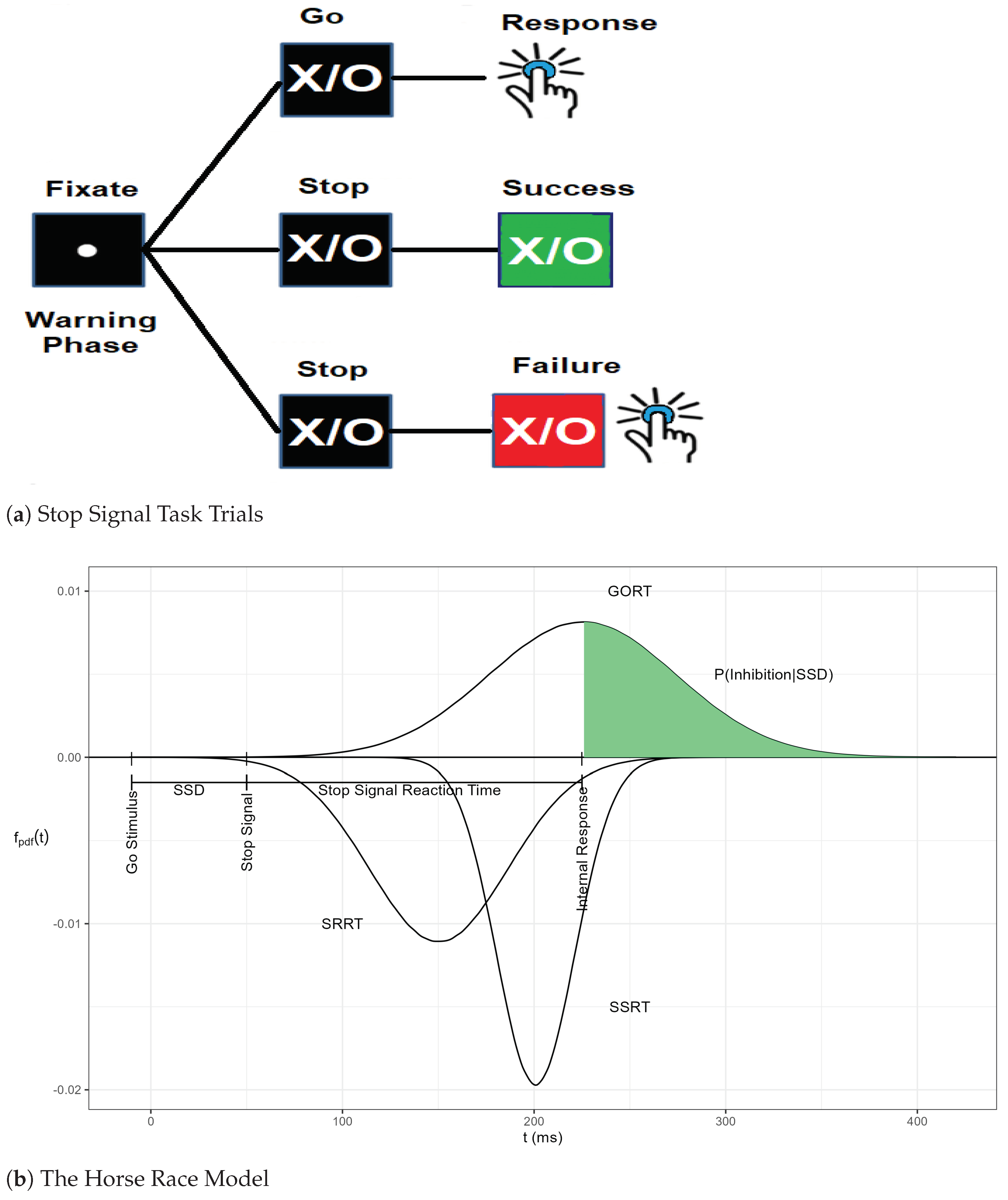
1.1. Stop Signal Task

The concept of “Response Inhibition” refers to the situations in which the current ongoing course of actions or thoughts must be changed, controlled, or stopped [1]. The inhibition can be either proactive or reactive [2,3], and the paradigms commonly used for its study are the go/no-go task (GNGT) [4] and the stop signal task (SST) [5,6,7]. The earliest model of the SST was proposed by Vince in 1948, and more complete versions were proposed in the following decades for two-choice tasks, go and stop trials [7,8]. The experiment starts with a fixation period on the computer screen. In the go tasks, a random series of X or O symbols are shown to the participant on the computer screen. The participant is then instructed to press the correct gamepad button associated with either X or O. Approximately 25% (i.e., probability of stop signal delay $p_{ss}=0.25$) of these trials have a stop signal after taking a short time of delay, which is called a stop signal delay time (SSD). The participant is instructed with an auditory beep sign to withhold pressing the game device buttons. The outcome from stop trials is categorized into one of successful inhibition (i.e., withholding pressing the device button) or failed inhibition (i.e., already have been pressing the device). Figure 1a presents the stop signal task.

The stop signal task has been proposed through four methods: the deadline model [9], the independent horse race model [10], the interactive horse race model [11], and the Hanes–Carpenter model [12]. We focus on the independent horse race model in details in the next section and its generalized non-independent version.

1.2. The Horse Race Model

The race model is founded on the notion of the race between two go process (GORT) and the stop process (SSRT) that is initiated upon triggering stop signal delay (SSD). Here, if $GORT>SSD+SSRT,$ then a successful inhibition of the primary go task is executed. Otherwise, a failed inhibition of the primary go task is recorded. The GORT in this type of trial is called the signal respond reaction times (SRRT). Figure 1b illustrates the complete independent horse race model. There are three presumptions:

First, there is stochastic independency (Stoch. Ind.) where GORT in go trials and SSRT in stop trials are independent (i.e., GORT ⊥ SSRT).

Second, there is contextual independency where GORT in go trials and GORT in stop trials have the same distribution (i.e., $GORT\stackrel{d}{=}\left(GORT\right|SSD)$).

Third, there is a non-constant status for SSRT as a random variable.

We refer to the general non-independent horse race model as a complete horse race model in which the assumption of the stochastic independency of GORT and SSRT processes is relaxed. Since a non-zero Spearman correlation implies statistical dependence, [13] (Proposition 7.1.3(i)), we will quantify the dependence of GORT and SSRT in terms of their non-zero Spearman correlation.

The entire distribution of SSRT can be modeled with non-parametric Frequentist methods [14] or Bayesian Parametric Approaches (BPA) with various features such as Individual BPA (IBPA) and Hierarchical BPA (HBPA) [15] and mixture methods [16]. In the next section, we discuss two useful distributions to model GORT and SSRT: Exponentially modified Gaussian (ExG) and Shifted Wald (SW).

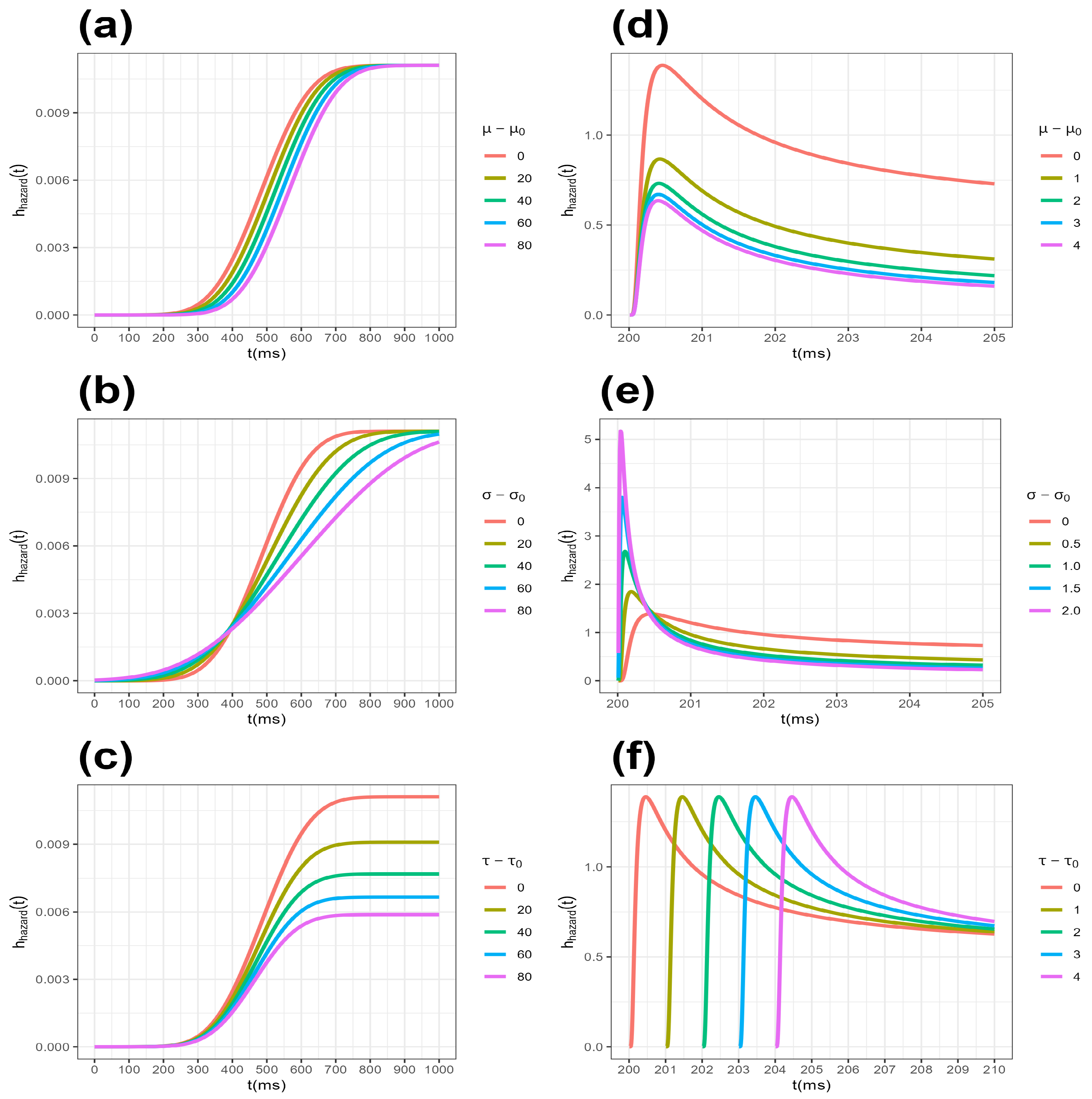
1.3. The Key Reaction Times Distributions

Distributions proposed to model reaction time can be grouped into two families [17,18,19,20,21,22,23,24,25]. One is the family of convolutionary distributions such as Exponentially modified Gaussian (ExG) and Exponentially modified Wald (ExW) [19,20]. The other is the family of non-convolutionary distributions such as Gumbel, Weibull, Lognormal, Gamma and Shifted Wald (SW) distributions [21,22,23,24,25]. Our work in this paper focuses on the ExG distribution from the convoluntionary family with a monotonically increasing hazard function and the SW distribution from the non-convolutionary family with a peaked hazard function.

Table 1. A summary of Exponentially modified Gaussian (ExG) and Shifted Wald (SW) distributions’ key features.

Distribution	$\mathbf{ExG}(\mathit{\mu },\mathit{\sigma },\mathit{\tau })$	$\mathbf{SW}(\mathit{\mu },\mathit{\sigma },\mathit{\tau })$
Representation	$N(\mu ,{\sigma }^2)\oplus Exp\left(\tau \right)$	$Wald(\mu ,{\sigma }^2)\oplus {\delta }_{\tau }$
Domain	$t\in \mathbb{R}$	$t\in {\mathbb{R}}_{\tau }^{+}$
Parameters	$\mu \in \mathbb{R},\sigma \in {\mathbb{R}}^{+},\tau \in {\mathbb{R}}^{+}$	$\mu \in {\mathbb{R}}^{+},\sigma \in {\mathbb{R}}^{+},\tau \in {\mathbb{R}}_0^{+}$
PDF	$\frac{1}{\tau }exp(-\frac{t-\mu }{\tau }+\frac{{\sigma }^2}{2{\tau }^2})\mathsf{\Phi }(\frac{t-\mu }{\sigma }-\frac{\sigma }{\tau })$	$\frac{1}{\sqrt{2\pi }\sigma {(t-\tau )}^{\frac{3}{2}}}exp(-\frac{{(t-\tau -\mu )}^2}{2{\sigma }^2{\mu }^2(t-\tau )})$
CDF	$\mathsf{\Phi }\left(\frac{t-\mu }{\sigma }\right)-exp(-\frac{t-\mu }{\tau }+\frac{{\sigma }^2}{2{\tau }^2})\mathsf{\Phi }(\frac{t-\mu }{\sigma }-\frac{\sigma }{\tau })$	$\mathsf{\Phi }\left(\frac{t-\tau -\mu }{\sigma \mu \sqrt{t-\tau }}\right)+exp\left(\frac{2}{\mu {\sigma }^2}\right)\mathsf{\Phi }\left(\frac{-(t-\tau )-\mu }{\sigma \mu \sqrt{t-\tau }}\right)$
Mean	$\mu +\tau$	$\mu +\tau$
Variance	${\sigma }^2+{\tau }^2$	${\mu }^3{\sigma }^2$
Skewness	$2{\sigma }^{-3}{\tau }^3{(1+{\sigma }^{-2}{\tau }^2)}^{\frac{-3}{2}}$	$3{\left(\mu {\sigma }^2\right)}^{\frac{1}{2}}$
Kurtosis	$3(1+2{\sigma }^{-2}{\tau }^2+3{\sigma }^{-4}{\tau }^4){(1+{\sigma }^{-2}{\tau }^2)}^{-2}$	$15\mu {\sigma }^2+3$
Hazard Function	↗	↷

Note: Φ is the CDF of the standard normal distribution.

presents key information regarding ExG and SW distributions.

Note that both ExG and SW are three parametric, right-skewed, leptokurtic, and, generally non-members of the exponential family. However, they differ in terms of domains and functional behaviors. For example, ExG is defined on all real values, while SW is defined on only non-negative real values (or real values not smaller than $\tau \ge 0$). In addition, the ExG hazard function is monotonically increasing, while the SW hazard function is peaked at some values in the domain. Figure 2 presents these distributions hazard function behaviors under a variety of scenarios of their associated parameter changes.

1.4. Motivation

Until the early 2020s, several studies have tested various hypotheses in the stop signal paradigm concerning inhibition functions, the validity of assumptions of the horse race model, and a new index estimation of SSRT using simulations [26,27,28,29,30,31,32]. One may find the codes used for the simulations of the stop signal task in C [26], Matlab [27], R [28,29,30], and Python [31,32]. However, the authors believe further improvement is needed for the following reasons.

First, based on our literature review, we could not find a standalone statistical software package that allows researchers to simulate the stop signal task data effectively, easily, and timely.

Second, the scripts noted above are based on the assumptions that conceptualize the go-and-stop processes using the ExG distribution, which violates peak hazard behavior observed in many empirical reaction times. This violation ultimately restricts the use of their implementations.

Third, either fixed SSD or the tracking methods are written in the scripts noted above—there are no tools allowing researchers to work simultaneously with both methods yet.

Fourth, the above methods all use an independent horse race model, yet no statistical software code has been proposed until now to simulate the generally non-independent horse race model.

Finally, R provides a flexible and rich environment to work with other data simulation packages successfully established in various medical fields, such as psychology and neuroscience [33,34,35,36,37,38]. In addition, the researchers can take advantage of open-source and free software across platforms with active community development [39,40].

Hence, the authors’ main motivation to present the R package, SimSST [41], available on CRAN is to enable the researchers to simulate the stop signal task data easier, freely, faster, more efficient, effectively, and with continuous community support.

1.5. Study Outline

This paper is organized as follows. We start by providing minimal but required theories and instructions for installing the SimSST package. The main functions simulating SST data with fixed SSD and tracking methods are then illustrated. Next, we present a simulation study for estimating the parameters used in distributions of modeling GORT and SSRT using the package. Finally, we discuss the contribution of the SimSST package to the stop signal task study, current limitations, and future development plans.

2. The SimSST Package

2.1. The Background and Installation

The “SimSST” package is based on the general non-independent horse-race model. Each round of simulations is carried out with the following steps:

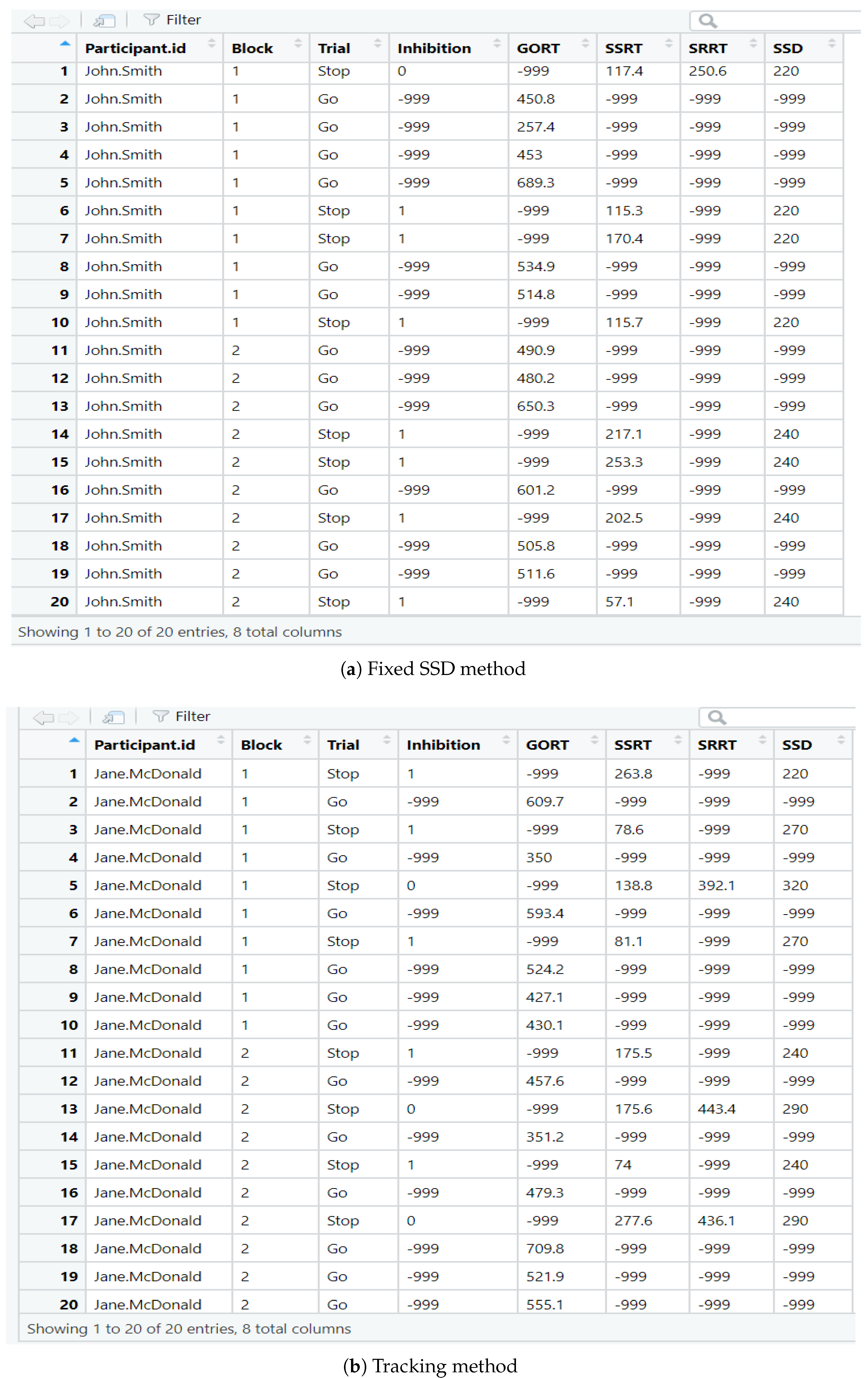
• Set the simulation method (fixed SSD or tracking).
• Set the stochastic independency status of GORT and SSRT processes (Yes or No).
• Set distribution type for GORT and SSRT and also set starting SSD (one of seven distributions: ExW, ExG, SW, Gumbel, Weibull, Lognormal and Gamma).
• Simulate each process (either independently or using Copulas).
• Test if the response from the first stop trial meets $SSRT+SSD<GORT$. If so, the trial is marked as successful inhibition. Otherwise, failed inhibition.
• Test and record the status of all successive stop trials.

  (a)

  Fixed SSD Method—Repeat checking if the following stop trial status is similar to the first one without a change in the value of SSD in each stop trial.

  (b)

  Tracking Method—Check the status of the first stop trial. If a stop is successful, add a redesigned constant d (e.g., 50 ms) to the SSD to check the status of the second stop trial. Otherwise, subtract d (e.g., 50 ms) from the SSD to check that trial status. Repeat this algorithm for the successive stop trials until the end.

The simulation process presented above may involve 2 × 2 × $7^2=196$ potential scenarios.

Table 2. A summary of potential simulation scenarios by R package “SimSST” (version 0.0.5.2).

Scenario	Method	Stoch. Ind.	GORT	SSRT	Function
1	Fixed SSD	Yes	ExG	ExG	simssfixed()/simssgen()
2				SW	simssfixed()/simssgen()
3			SW	ExG	simssfixed()/simssgen()
4				SW	simssfixed()/simssgen()
5		No	ExG	ExG	simssgen()
6				SW	simssgen()
7			SW	ExG	simssgen()
8				SW	simssgen()
9	Tracking	Yes	ExG	ExG	simsstrack()/simssgen()
10				SW	simsstrack()/simssgen()
11			SW	ExG	simsstrack()/simssgen()
12				SW	simsstrack()/simssgen()
13		No	ExG	ExG	simssgen()
14				SW	simssgen()
15			SW	ExG	simssgen()
16				SW	simssgen()

presents sixteen (2 × 2 × $2^2=16$) scenarios offered by the package SimSST (version 0.0.5.2).

The package “SimSST” depends on three R packages: “gamlss.dist” [42], “MASS” [43], and, “dplyr” [44], and it was developed under R-4.1.3 [45]. The package (version 0.0.5.2) is available from the Comprehensive R Archive Network (CRAN) at https://CRAN.R-project.org/package=SimSST (accessed on 9 January 2023). The following code chunk shows how to install and load the package:

line #1:> install.packages("SimSST", dependencies=TRUE)

line #2:> library(SimSST)

The “SimSST” package involves three major multi-variate functions simssfixed(), simsstrack() and simssgen(). The first two are based on an independent horse-race model, and the third one is based on a general non-independent horse-race model. Details are described in the coming sections. The reader may try to type ?simssfixed, ?simsstrack or ?simssgen in R for the details.

2.2. The Fixed SSD Based Simulated SST Data

The function simssfixed() simulates the SST data based on the independent horse race model and the fixed SSDs and needs the following nine input parameters to simulate SST data. For given $b\ge 1$, id is a b-sized character vector for participants’ IDs. The parameters block, n, and m are b-sized numeric vectors of block numbers, total trials per block, and stop trials per block, respectively. SSD.b is a b-sized vector of initial stop signal delays on each block. The dist.go and theta.go parameters are b-sized character vectors, specifying the type of GORT distributions, and a $b\times 3$ numeric matrix having the specification of their distributions, respectively. Similarly, dist.stop and theta.stop are a b-sized numeric vector specifying the type of SSRT distributions and a $b\times 3$ numeric matrix having the specification of their distributions. The function general code in R is:

simssfixed(pid,block,n,m,SSD.b,dist.go,theta.go,dist.stop,theta.stop)

2.3. The Tracking Method Based Simulated SST Data

The function simsstrack() similarly simulates the SST data based on the independent horse race model and the tracking method in which at each stage a constant of 50 ms is added or subtracted to the following SSDs. Its parameters are the same as those of the former function simssfixed() and its code in R is the following:

simsstrack(pid,block,n,m,SSD.b,dist.go,theta.go,dist.stop,theta.stop)

2.4. The General Tracking Method Based Simulated Correlated SST Data

The functions simssfixed() and simsstrack() proposed in the package “SimSST” have two limitations. First, both are based on the stochastic independence of GORT and SSRT processes. Recent studies have shown a severe violation of the assumptions needed for the independent horse race paradigm [46]. Solutions to overcome this issue are considering SSDs from 200 ms and incorporation of the Spearman’s rank correlation [47] for the case of the relaxation of the assumption of stochastic independence between GORT and SSRT. (Note that for simulation purposes, the Pearson correlation is an inappropriate parameter as it may not be preserved under monotonic transformations of the original simulated data [47].) Second, there is no mechanism to connect the functions simssfixed() and simsstrack(). In particular, we know that replacing the constant added (subtracted) value of 50 ms to the SSD in the subsequent stop trials with 0 converts simsstrack() function to the simssfixed(). To solve these limitations, we may consider the generalized simulation function simssgen() based on the theory of copulas with eleven parameters as follows:

simssgen(pid,block,n,m,SSD.b,dist.go,theta.go,dist.stop,theta.stop,rho,d)

where in which the first nine parameters are exactly as those in the functions simssfixed() and simsstrack() and the additional parameters $rho$ and d refer to b-sized numeric vectors of the Spearman correlation of GORT and SSRT processes and the b-sized numeric vectors of measure of added (subtracted) constant to the initial SSD values, respectively. In particular, denoting the first nine parameters with “−”, we will have:

$$\begin{array}{ccc}\hfill simssgen(-,rho={\left(0\right)}_{b\times 1},d={\left(0\right)}_{b\times 1})& =& simssfixed(-)\hfill \end{array}$$

(1)

$$\begin{array}{ccc}\hfill simssgen(-,rho={\left(0\right)}_{b\times 1},d={\left(50\right)}_{b\times 1})& =& simsstrack(-).\hfill \end{array}$$

(2)

As the first working example for the fixed SSD-based simulated SST data, let us consider a participant John Smith for two rounds (i.e., blocks) of stop signal task trials, each of size ten trials, including four random stop trials. We assume that for these rounds of SST trials, the initiating stop signal delays are 220 ms and 240 ms, respectively. A further assumption is that the GORT and SSRT are independently distributed as $ExG(\mu =440,\sigma =90,\tau =90)$ and $ExG(\mu =120,\sigma =80,\tau =70)$, respectively. The R code given bellow produces the simulated dataset presented in Figure 3a (note that the probability of stop signal is given by $p_{ss}=m/n=0.40$):

line #1:> mySSTdata1<- simssgen(

               pid = c("John.Smith", "John.Smith"),

               block = c(1,2),

               n = c(10,10),

               m = c(4,4),

               SSD.b = c(220,240),

               dist.go = c("ExG", "ExG"),

               theta.go = as.matrix(rbind(c(440,90,90),c(440,90,90))),

               dist.stop = c("ExG", "ExG"),

               theta.stop = as.matrix(rbind(c(120,80,70),c(120,80,70))),

               rho=c(0,0),

               d=c(0,0))

line #2:> mySSTdata1

As the second working example for the tracking method-based simulated SST data, we now consider another participant called Jane McDonald with the same parameter specification used for the former participant, John Smith. Then, with given tracking method in which $d=+50$ ms, the R code given below produces Figure 3b:

line #1:> mySSTdata2<- simssgen(

               pid = c("Jane.McDonald", "Jane.McDonald"),

               block = c(1,2),

               n = c(10,10),

               m = c(4,4),

               SSD.b = c(220,240),

               dist.go = c("ExG", "ExG"),

               theta.go = as.matrix(rbind(c(440,90,90),c(440,90,90))),

               dist.stop = c("ExG", "ExG"),

               theta.stop = as.matrix(rbind(c(120,80,70),c(120,80,70))),

               rho=c(0,0),

               d=c(50,50))

line #2:> mySSTdata2

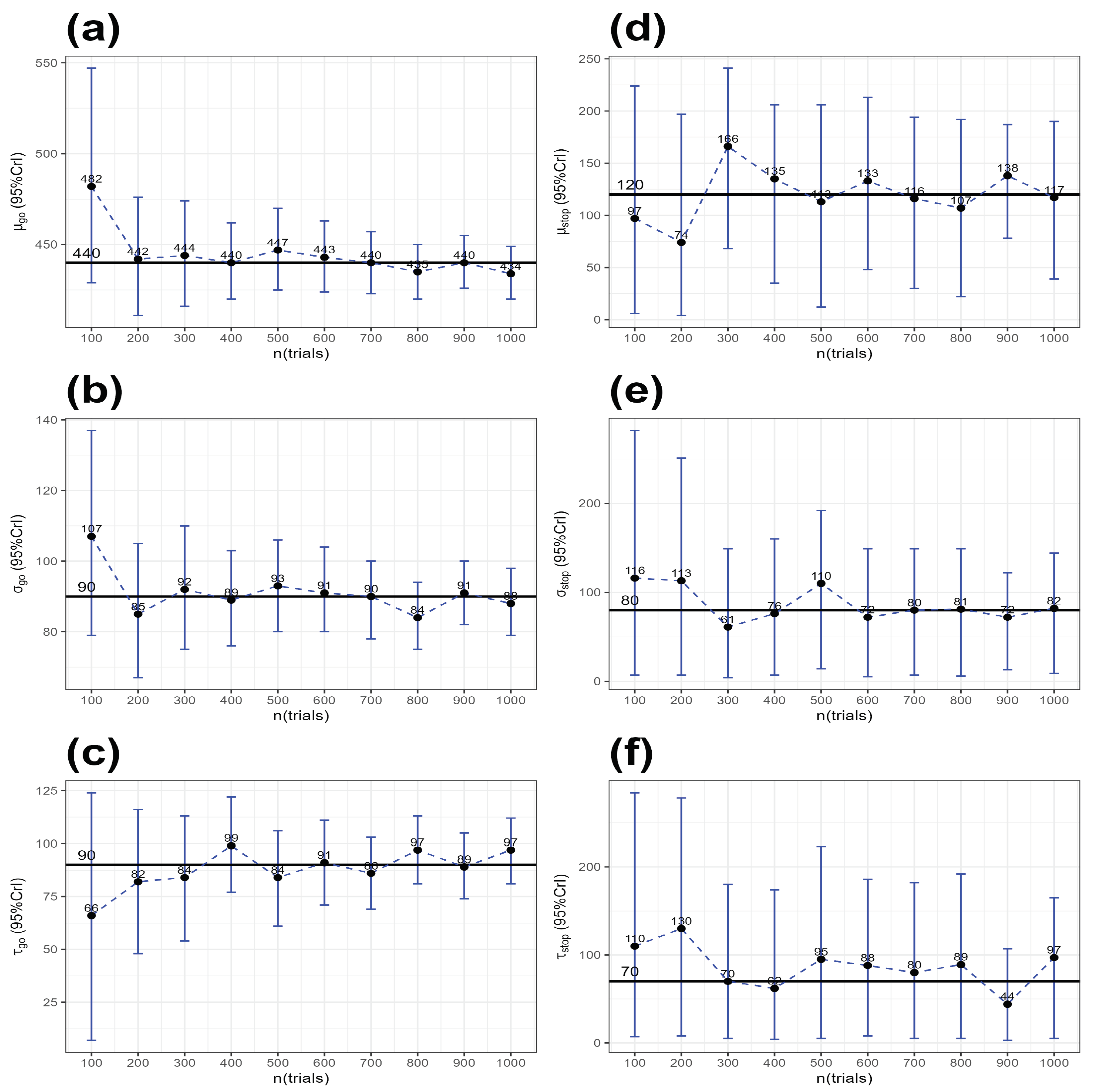
2.5. Simulation Study: An Example

This section provides an example (scenario #9 in Table 2) showing the analysis of SST trial data generated by the SimSST package. Consider a single participant for one block of trials with the following input parameters (we assume that the proportion of stop stimuli is $p_{ss}=m/n=0.25$).

Method:	Tracking
Stoch. Ind. Status:	Independent
Initial SSD:	220 ms
d parameter:	50 ms
total trials:	$n=100$ k $(1\le k\le 10)$
stop trials:	$m=25$ k $(1\le k\le 10)$
GORT distribution:	ExGaussian(ExG)
${\theta }_{go}=({\mu }_{go},{\sigma }_{go},{\tau }_{go})$	$(440,90,90)$
SSRT distribution:	ExGaussian(ExG)
${\theta }_{stop}=({\mu }_{stop},{\sigma }_{stop},{\tau }_{stop})$	$(120,80,70).$

We now generates the first of ten simulated data using the function simsstrack in the SimSST package.

line #1:> library(SimSST)

line #2:> SimSST_Data1 <- simssgen(

                pid = c("FNLN1"),

                block = 1,

                n = 100,

                m = 25,

                SSD.b = 220,

                dist.go = "ExG",

                theta.go = as.matrix(rbind(c(440,90,90))),

                dist.stop = "ExG",

                theta.stop = as.matrix(rbind(c(120,80,70))),

                rho=0,

                d=50)

line #3:> SimSST_Data1

After saving all ten datasets in .csv format, we convert them as input to the BEESTS software [48] with the following minor modifications: (i) Record positive SRRT values in the GORT column, (ii) Rename the columns of Trial, Inhibition, SSD and GORT to ss-presented, inhibited, ssd and rt, respectively, and (iii) Sort the dataset using the ss-presented column in ascending order. We provide the R code in Appendix A to avoid these tedious manual modifications. The reader can access the simulated datasets in the supplementary materials.

We now have the BEESTS formatted data for analysis. The following prior specification and MCMC setting are used to apply the standard BEESTS IBPA [15,48]:

Prior Setting Information:
${\mu }_{go}\sim Uniform[1,1000]:$	start value: 500
${\sigma }_{go}\sim Uniform[1,500]:$	start value: 150
${\tau }_{go}\sim Uniform[1,500]:$	start value: 150
${\mu }_{stop}\sim Uniform[1,1000]:$	start value: 300
${\sigma }_{stop}\sim Uniform[1,500]:$	start value: 150
${\tau }_{stop}\sim Uniform[1,500]:$	start value: 150
MCMC Setting Information:
Number of chains:	3
Samples:	50,000
Burn in:	5000
Thining:	5
Limits of Integration:	1–10,000
With Trigger Failure(WTF):	No.

Figure 4 shows each parameter estimate of GORT and SSRT with their 95% CrI fitted by the BEESTS IBPA. We confirmed that for all cases, the parameters used for generating the SST trial dataset are captured by the 95% CrI. Note that the estimation of the GORT parameters can generally be improved by increasing the total trial sample size, resulting in a narrower 95% CrI. On the other hand, estimating the parameters associated with SSRT generally produces a wider 95% CrI, and some oscillations for the ${\tau }_{stop}$ parameter are found.

Simulation performance is discussed using ten mean posterior estimates of each the six parameters $\theta \in ({\mu }_{go},{\sigma }_{go},{\tau }_{go},{\mu }_{stop},{\sigma }_{stop},{\tau }_{stop}).$ We tested $H_0:\theta ={\theta }_{0}vs.H_1:\theta \ne {\theta }_0$, where ${\theta }_0$ is the predefined true parameter value used for generating data, using one-sample t-test and one sample Wilcoxon signed-rank test. As reported in

Table 3. A summary of one sample t-test and one sample Wilcoxon signed-ranked test for each of individual parameters ($n=10$).

${\mathit{H}}_0:\mathit{\theta }={\mathit{\theta }}_0$
${\mathit{H}}_{\mathbf{1}}:\mathbf{\theta }\ne {\mathbf{\theta }}_{\mathbf{0}}$
$\mathbf{\theta }={\mathbf{\theta }}_{\mathbf{0}}$	${\mathbf{\mu }}_{\mathbf{go}}=\mathbf{440}$	${\mathbf{\sigma }}_{\mathbf{go}}=\mathbf{90}$	${\mathbf{\tau }}_{\mathbf{go}}=\mathbf{90}$	${\mathbf{\mu }}_{\mathbf{stop}}=\mathbf{120}$	${\mathbf{\sigma }}_{\mathbf{stop}}=\mathbf{80}$	${\mathbf{\tau }}_{\mathbf{stop}}=\mathbf{70}$
(a) t-test
$\widehat{\theta }(95\%CI)$	445(435,454)	91(86,96)	88(81,94)	120(102,138)	86(72,100)	86(69,104)
Sig.(2-sided)	0.305	0.629	0.436	0.961	0.332	0.061
PE(%)	1.1	1.1	2.2	0.0	7.5	22.9
(b) Wilcoxon test
$\widehat{\theta }(95\%CI)$	443(435,464)	90(87,98)	89(81,94)	120(102,138)	87(71,110)	89(66,110)
Sig.(2-sided)	0.447	0.953	0.721	1.000	0.635	0.076
PE(%)	0.7	0.0	1.1	0.0	8.8	27.1

Note: Percentage Error (PE) was calculated as $PE=|\widehat{\theta }-{\theta }_0/{\theta }_0|\times \mathrm{100\%}$.

, all six parameters are not significantly different from the one assumed given non-multiplicity (note that we have stronger evidence for non-significant results as well when controlling for multiplicity with Holm’s method for $m=6,$ [49]). However, relatively high PE values associated with the parameter ${\tau }_{stop}$ are shown in both tests. This result might be attributed to the small stop trials sample size and wider prior distributions specified in the BEESTS IBPA. This finding cautions the researchers to choose more informative stop priors than those used in the standard BEESTS IBPA.

3. Discussion

3.1. Summary and Contributions

We provide an R package, SimSST, which is the first statistical software package implementation of simulating stop signal task data since its concept was introduced in 1948. The package can simulate data (1) using either a fixed SSD or tracking method and/or (2) either stochastically independent or dependent GORT and SSRT processes and/or (3) either monotone increasing hazard or peaked hazard reaction times distribution describing GORT and SSRT processes. In addition, flexibility on controlling the number of stop trials and total trials allows researchers to explore the asymptotic property through testing the hypothesis. We anticipate that the package assists the researchers to simulate SST under various conditions using a general non-independent horse race paradigm efficiently. As an application, one may simulate SST data under various scenarios and investigates its connection to fMRI-EEG data to investigate the missing angles of the associated results to the empirical data in the past studies [50].

3.2. Limitations and Future Work

Our work has several limitations, but they are taken as new perspectives for extensions as follows:

First, the current version of the SimSST package supports a limited number of distributions, such as ExG and SW for a three-parameter family of distributions. The key two parametric candidates such as Weibull, Gamma, and Lognormal [51] need inclusion. One may ask to include an Exponentially modified Wald (ExW) distribution [52] for the three-parameter family for the next version.

Second, the package “SimSST” does not yet a address simulation trials with trigger failures (TF). This issue creates another dimension for its extension in the subsequent version.

Third, the scope of a simulation study using the SimSST package depends on the current support of BEESTS software. For example, BEESTS does not include SW distributional assumption. This limits parameter estimations scenarios.

Fourth, the illustrative example with this SimSST package is based on one participant with a single block trial with various sizes of trials. The extension of this example to the case with several participants (each with several blocks of trials) needs investigation. The implementation of this scenario requires the hierarchical Bayesian parametric approach (HBPA) supported by BEESTS.

Aside from the above four potential future work directions, there is another potential future work direction through the presented simulations in the SimSST package: investigation of behavior of inhibition function $P\left(Inhibition\right|SSD)$ (Figure 1b) in terms of relative position of GORT and SSRT processes when they are simulated from the same parametric distributions [53]. Here, given scenarios 1, 4, 5, 8, 9, 12, 13 and 16 in Table 2, it is plausible to explore the behavior of the inhibition function when the GORT process is weakly faster or strongly faster (or none) versus the SSRT process. A final classification of models of response inhibition over these results [54] and across a spectrum of clinical groups will widen our understanding of the underlying brain inhibition processes.

3.3. Conclusions

The free SimSST R package enables one to simulate stop signal task data under a generally non-independent horse race paradigm, ExG and SW parametric assumptions for the GORT/SSRT processes and both fixed SSD and tracking methods. The simulated datasets help researchers test their plausible hypothesis regarding various stopping processes within the stop signal task literature. This saves researchers the required time and costs associated to the empirical SST data.

References

1. Schachar, R.J.; Logan, G.D.; Robaey, P.; Chen, S.; Ickowicz, A.; Barr, C. Restraint and Cancellation: Multiple Inhibition Deficits in Attention Deficit Hyperactivity Disorder. J. Abnorm. Child Psychol. 2007, 35, 229–238. [Google Scholar] [CrossRef] [PubMed]
2. van den Wildenberg, W.P.M.; Ridderinkhof, K.R.; Wylie, S.A. Towards Conceptual Clarification of Proactive Inhibitory Control: A Review. Brain Sci. 2022, 12, 1638. [Google Scholar] [CrossRef] [PubMed]
3. Soltanifar, M.; Escobar, M.; Dupuis, A.; Chevrier, A.; Schachar, R. The Asymmetric Laplace Gaussian (ALG) Distribution as the Descriptive Model for the Internal Proactive Inhibition in the Standard Stop Signal Task. Brain Sci. 2022, 12, 730. [Google Scholar] [CrossRef] [PubMed]
4. Trommer, B.L.; Hoeppner, J.B.; Lorber, R.; Armstrong, K.J. The Go-No-Go Paradigm in Attention Deficient Disorder. Ann. Neurol. 1988, 24, 610–614. [Google Scholar] [CrossRef] [PubMed]
5. Logan, G.D.; Cowan, W.B. On the Ability to Inhibit Thought and Action: A Theory of an Act of Control. Psychol. Rev. 1984, 91, 295–327. [Google Scholar] [CrossRef]
6. Verbruggen, F.; Aron, A.R.; Band, G.H.; Beste, C.; Bissett, P.G.; Brockett, A.T.; Brown, J.W.; Chamberlain, S.R.; Chambers, C.D.; Colonius, H.; et al. A consensus guide to capturing the ability to inhibit actions and impulsive behaviors in the stop-signal task. eLife 2019, 8, e46323. [Google Scholar] [CrossRef]
7. Logan, G.D.; van Zandt, T.; Verbruggen, F.; Wagenmakers, E.J. Ability to Inhibit Thought and Action: General and Special Theories of an Act of Control. Psychol. Rev. 2014, 121, 66–95. [Google Scholar] [CrossRef] [Green Version]
8. Vince, M.A. The intermittency of control movements and the psychological refractory period. Br. J. Psychology. Gen. Sect. 1948, 38, 149–157. [Google Scholar]
9. Ollman, R.T.; Billington, M.J. The Deadline Model for Simple Reaction Times. Cogn. Psychol. 1972, 3, 311–336. [Google Scholar] [CrossRef]
10. Logan, G.D. Attention, Automaticity, and the Ability to Stop a Speeded Choice Response. In Attention and Performance IX; Long, J., Baddeley, A.D., Eds.; Hillsdale: Erlbaum, NJ, USA, 1981. [Google Scholar]
11. Boucher, L.; Palmeri, T.J.; Logan, G.D.; Schall, J.D. Inhibitory Control in Mind and Brain: An Interactive Race Model of Countermanding Saccades. Psychol. Rev. 2007, 114, 376–397. [Google Scholar] [CrossRef] [Green Version]
12. Hanes, D.P.; Carpenter, R.H.S. Countermanding Saccades in Humans. Vis. Res. 1999, 39, 2777–2791. [Google Scholar] [CrossRef] [PubMed]
13. Athreya, K.B.; Lahiri, S.M. Measure Theory and Probability Theory; Springer: New York, NY, USA, 2006. [Google Scholar]
14. Colonius, H. A Note on the Stop Signal Paradigm, or How to Observe the Unobservable. Psychol. Rev. 1990, 97, 309–312. [Google Scholar] [CrossRef]
15. Matzke, D.; Dolan, C.V.; Logan, G.D.; Brown, S.D.; Wagenmakers, E.J. Bayesian Parametric Estimation of Stop signal Reaction Time Distributions. J. Exp. Psychol. Gen. 2013, 142, 1047–1073. [Google Scholar] [CrossRef] [PubMed]
16. Soltanifar, M.; Escobar, M.; Dupuis, A.; Schachar, R. A Bayesian Mixture Modelling of Stop Signal Reaction Time Distributions: The Second Contextual Solution for the Problem of Aftereffects of Inhibition on SSRT Estimations. Brain Sci. 2021, 11, 1102. [Google Scholar] [CrossRef]
17. Del Prado Martin, F.M. A Theory of Reaction Times Distributions. 2008. (Unpublished). Available online: http://cogprints.org/6310 (accessed on 16 December 2022).
18. Palmer, E.M.; Horowitz, T.S.; Torralba, A.; Wolfe, J.M. What are the Shapes of Response Times Distributions in Visual Search? J. Exp. Psychol. 2011, 37, 58–71. [Google Scholar] [CrossRef] [Green Version]
19. Heatcote, A. RTSYS: A DOS Application for the Analysis of Reaction Times Data. Behav. Res. Methods Instrum. Comput. 1996, 28, 427–445. [Google Scholar] [CrossRef]
20. Schwarz, W. The Ex-Wald Distribution as a Descriptive Model of Reaction Time Data. Behav. Res. Methods Instruments Comput. 2001, 33, 457–469. [Google Scholar] [CrossRef] [Green Version]
21. Gumbel, E.J. The Statistics of Extremes; Columbia University Press: New York, NY, USA, 1958. [Google Scholar]
22. Weibull, W. A Statistical Distribution Function of wide Applicability. J. Appl. Mech. Transform. ASME 1951, 18, 293–297. [Google Scholar] [CrossRef]
23. Johnson, N.L.; Kotz, S.; Balakrishnan, N. Continuous Univariate Distributions, 2nd ed.; “14: Lognormal Distributions”; John Wiley & Sons: New York, NY, USA, 1994; Volume 1. [Google Scholar]
24. Lancaster, H.O. Forerunners of the Pearson chi-square. Aust. J. Stat. 1966, 8, 117–126. [Google Scholar] [CrossRef]
25. Royce, A.; Alario, F.X.; Van Maanen, L. The Shifted Wald Distribution for Response Time Data Analysis. Psychol. Methods 2016, 21, 309–327. [Google Scholar]
26. Band, G.P.; van der Molen, M.W.; Logan, G.D. Horse-race model simulations of the stop-signal procedure. Acta Psychol. 2003, 112, 105–142. [Google Scholar] [CrossRef] [PubMed]
27. Hannah, R.; Muralidharan, V.; Aron, A.R. Failing to attend versus failing to stop: Single-trial decomposition of action-stopping in the stop signal task. Behav. Res. Methods 2022, 1–19. [Google Scholar] [CrossRef]
28. Weise, L.; Boecker, M.; Gauggel, S.; Falkenburger, B.; Drueke, B. A reaction-time adjusted PSI method for estimating performance in the stop-signal task. PLoS ONE 2018, 13, e0210065. [Google Scholar] [CrossRef] [PubMed]
29. Soltanifar, M.; Dupuis, A.; Schachar, R.; Escobar, M. A frequentist mixture modelling of stop signal reaction times. Biostat. Epidemiol. 2019, 3, 90–108. [Google Scholar] [CrossRef]
30. Soltanifar, M.; Knight, K.; Dupuis, A.; Schachar, R.; Escobar, M. A Time Series-Based Point Estimation of Stop Signal Reaction Times: More Evidence on the Role of Reactive Inhibition-Proactive Inhibition Interplay on the SSRT Estimations. Brain Sci. 2020, 10, 598. [Google Scholar] [CrossRef] [PubMed]
31. Ye, W. Dynamics of a revised neural mass model in the stop-signal task. Chaos Solitons Fractals 2020, 139, 110004. [Google Scholar] [CrossRef]
32. Bissett, P.G.; Hagen, M.P.; Jones, H.M.; Poldrack, R.A. Design issues and solutions for stop-signal data from the Adolescent Brain Cognitive Development (ABCD) study. ELife 2021, 10, e60185. [Google Scholar] [CrossRef]
33. Nieuwoudt, C.; Brooks-Wilson, A.; Graham, J. SimRVSequences. an R package to simulate genetic sequence data for pedigrees. Bioinformatics 2020, 36, 2295–2297. [Google Scholar] [CrossRef]
34. Tripathi, S.; Lloyd-Price, J.; Ribeiro, A.; Yli-Harja, O.; Dehmer, M.; Emmert-Streib, F. sgnesR: An R package for simulating gene expression data from an underlying real gene network structure considering delay parameters. BMC Bioinform. 2017, 18, 325. [Google Scholar] [CrossRef] [Green Version]
35. Nilforooshan, M.A. pedSimulate – An R package for simulating pedigree, genetic merit, phenotype, and genotype data. Rev. Bras. De Zootec. 2022, 51, e20210131. [Google Scholar] [CrossRef]
36. Technow, F.R. Package hypred: Simulation of Genomic Data in Applied Genetics. Ph.D. Thesis, University of Hohenheim, Institute of Plant Breeding, Seed Science and Population Genetics, Stuttgart, Germany, 2011. [Google Scholar]
37. Brilleman, S.L.; Wolfe, R.; Moreno-Betancur, M.; Crowther, M.J. Simulating Survival Data Using the simsurv R Package. J. Stat. Softw. 2021, 97, 1–27. [Google Scholar] [CrossRef]
38. Welvaert, M.; Durnez, J.; Moerkerke, B.; Verdoolaege, G.; Rosseel, Y. neuRosim: AnRPackage for Generating fMRI Data. J. Stat. Softw. 2011, 44, 1–19. [Google Scholar] [CrossRef]
39. Hackenberger, B.K. R software: Unfriendly but probably the best. Croat. Med. J. 2020, 61, 66–68. [Google Scholar] [CrossRef] [PubMed] [Green Version]
40. Mizumoto, A.; Plonsky, L. R as a Lingua Franca: Advantages of Using R for Quantitative Research in Applied Linguistics. Appl. Linguist. 2015, 37, 284–291. [Google Scholar] [CrossRef] [Green Version]
41. Soltanifar, M.; Lee, C. SimSST: Simulated Stop Signal Task Data. R Package Version 0.0.5.2. 2023. Available online: https://CRAN.R-project.org/package=SimSST (accessed on 9 January 2023).
42. Stasinopoulos, M.; Rigby, R. gamlss.dist: Distributions for Generalized Additive Models for Location Scale and Shape. R Package Version 6.0-5. 2022. Available online: https://CRAN.R-project.org/package=gamlss.dist (accessed on 9 January 2023).
43. Venables, W.N.; Ripley, B.D. Modern Applied Statistics with S., 4th ed.; Springer: New York, NY, USA, 2002; ISBN 0-387-95457-0. [Google Scholar]
44. Wickham, H.; François, R.; Henry, L.; Müller, K. dplyr: A Grammar of Data Manipulation. R Package Version 1.0.10. 2022. Available online: https://CRAN.R-project.org/package=dplyr (accessed on 9 January 2023).
45. R Core Team. R: A Language and Environment for Statistical Computing; R Foundation for Statistical Computing: Vienna, Austria, 2022; Available online: https://www.R-project.org/ (accessed on 9 January 2023).
46. Bissett, P.G.; Jones, H.M.; Poldrack, R.A.; Logan, G.D. Severe violations of independence in response inhibition tasks. Sci. Adv. 2021, 7, eabf4355. [Google Scholar] [CrossRef]
47. Wicklin, R. Simulating Data with SAS, 1st ed.; SAS Institute Inc.: Cary, NC, USA, 2013; pp. 169–174. [Google Scholar]
48. Matzke, D.; Love, J.; Wiecki, T.V.; Brown, S.D.; Logan, G.D.; Wagenmakers, E.J. Release the BEESTS: Bayesian Estimation of Ex-Gaussian Stop Signal Reaction Time Distributions. Front. Psychol. 2013, 4, 918. [Google Scholar] [CrossRef] [Green Version]
49. Holm, S. A Simple Sequentially Rejective Multiple Test Procedure. Scand. J. Stat. 1979, 6, 65–70. [Google Scholar]
50. Ko, L.-W.; Shih, Y.-C.; Chikara, R.K.; Chuang, Y.-T.; Chang, E.C. Neural Mechanisms of Inhibitory Response in a Battlefield Scenario: A Simultaneous fMRI-EEG Study. Front. Hum. Neurosci. 2016, 10, 1–15. [Google Scholar] [CrossRef] [Green Version]
51. Rouder, J.F. Are Un-shifted Distributional Models Appropriate for Response Time? Psychometrica 2005, 70, 377–381. [Google Scholar] [CrossRef]
52. Heathcote, A. Fitting Wald and ex-Wald distributions to response time data: An example using functions for the S-PLUS package. Behav. Res. Methods Instruments Comput. 2004, 36, 678–694. [Google Scholar] [CrossRef] [Green Version]
53. Soltanifar, M. A Look at the Primary Order Preserving Properties of Stochastic Orders: Theorems, Counterexamples and Applications in Cognitive Psychology. Mathematics 2022, 10, 4362. [Google Scholar] [CrossRef]
54. Verbruggen, F.; Logan, G.D. Models of response inhibition in the stop-signal and stop-change paradigms. Neurosci. Biobehav. Rev. 2009, 33, 647–661. [Google Scholar] [CrossRef] [PubMed]
Figure 1. (a) The standard stop signal task; (b) Graphical representation of the complete horse race model: GORT: go reaction times, SRRT: signal respond reaction times, SSRT: stop signal reaction times, S S D : stop signal delay.
Mathematics 11 00500 g001
Figure 2. (ac) ExG distribution hazard function change by parameters given μ 0 = 440 , σ 0 = 90 , τ 0 = 90 ; (df) SW distribution hazard function change by parameters given μ 0 = 1 , σ 0 = 1 , τ 0 = 200 .
Mathematics 11 00500 g002
Figure 3. Sample SimSST R software package(R studio version 4.1.3) simulated SST data output with input variables as in the text.
Mathematics 11 00500 g003
Figure 4. BEETS method parameters estimations for the SimSST-based simulated SST data with true parameter values on the black horizontal line: (ac) GORT ExG parameters; (df) SSRT ExG parameters.
Mathematics 11 00500 g004