
Peak-to-Peak Stabilization of Sampled-Data Systems Subject to Actuator Saturation and Its Practical Application to an Inverted Pendulum

Abstract
:1. Introduction
- Note that the current time can be represented as two consecutive sampling times by utilizing additional time-varying parameters. By introducing two novel time integrals of the weighted state derivative, this paper makes the initial attempt to incorporate these parameters into the augmented state. This inclusion enables the utilization of the sawtooth-type characteristics of time-varying parameters during the stability analysis process. Furthermore, the proposed time integrals of the weighted state derivative play a crucial role in constructing an improved looped-functional that can contain a greater amount of system state information between two consecutive sampling times.
- In contrast to [8,9,15], this paper provides two additional zero-equalities that can improve the relationship among components of the augmented state, resulting in less conservative stabilization conditions. By reducing the number of zero-equalities, the proposed method offers the advantage of lowering the overall computational complexity owing to the utilization of fewer slack variables.
- In contrast to other existing studies that address the stabilization problem of SDSs with energy-bounded disturbances, this paper presents a set of stabilization conditions based on linear matrix inequalities (LMIs). These conditions ensure that the closed-loop sampled-data system achieves exponential stability and guarantees a peak-to-peak performance within the domain of attraction (DoA). Additionally, to design a practical sampled-data controller for IPSs, the actuator saturation constraint is also considered in this paper.
2. Problem Formulation
- System (6) is exponentially stable in the absence of disturbances .
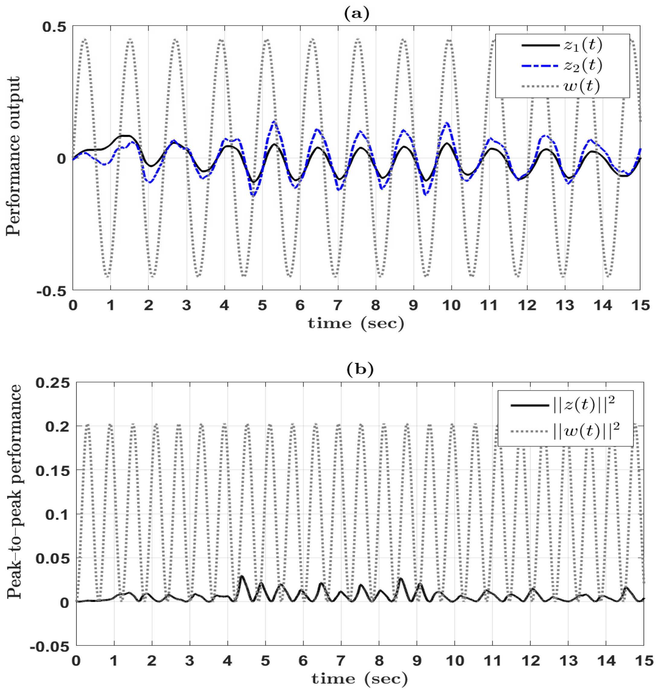
- For a prescribed scalar , an initial condition , and any non-zero disturbances , the performance output satisfies
3. Main Results
3.1. Stability Analysis
3.2. Stabilization Criteria
4. Numerical Validation
4.1. Comparison Examples
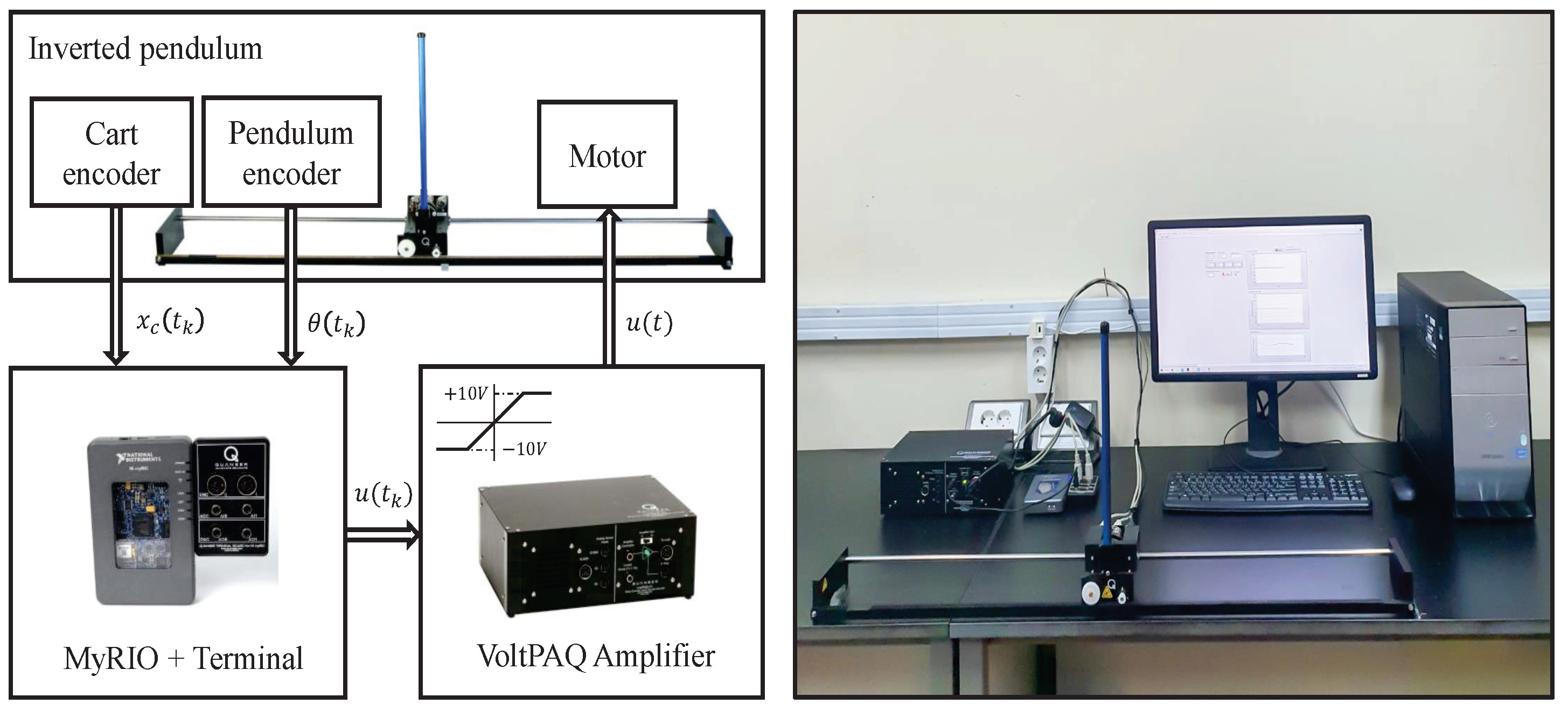
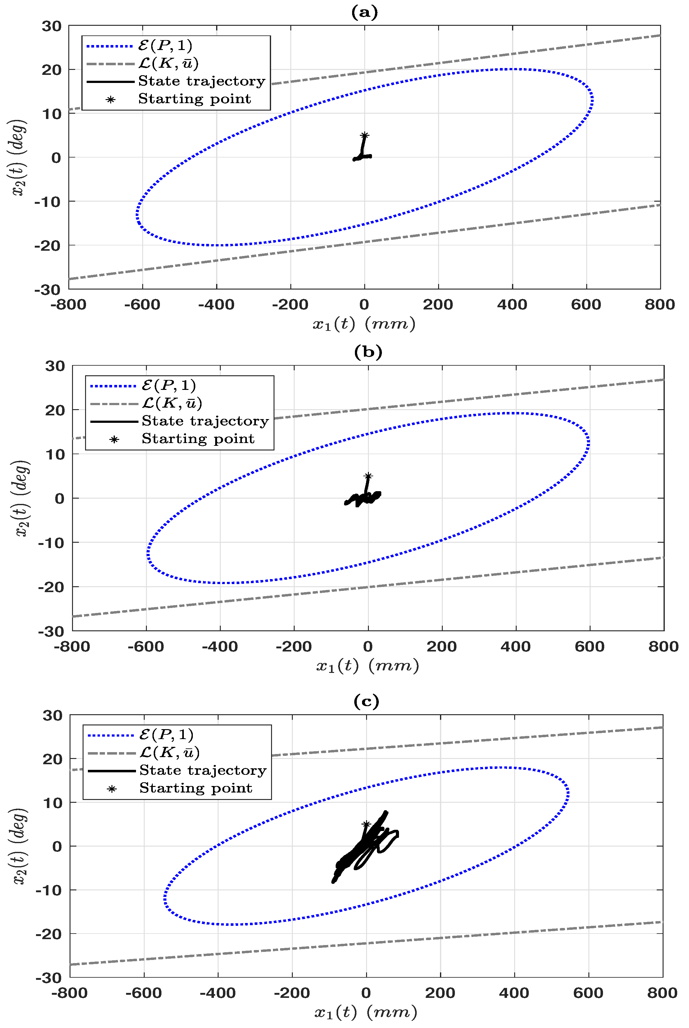
4.2. Application to Inverted Pendulum System
5. Conclusions
Author Contributions
Funding
Data Availability Statement
Conflicts of Interest
References
- Lee, T.H.; Park, J.H. New methods of fuzzy sampled-data control for stabilization of chaotic systems. IEEE Trans. Syst. Man Cybern.-Syst. 2017, 48, 2026–2034. [Google Scholar] [CrossRef]
- Lv, X.; Li, X. Finite time stability and controller design for nonlinear impulsive sampled-data systems with applications. ISA Trans. 2017, 70, 30–36. [Google Scholar] [CrossRef] [PubMed]
- Nguyen, K.H.; Kim, S.H. Improved sampled-data control design of T-S fuzzy systems against mismatched fuzzy-basis functions. Appl. Math. Comput. 2022, 428, 127150. [Google Scholar] [CrossRef]
- Nguyen, K.H.; Kim, S.H. Improved stability and stabilization criteria of sampled-data control systems based on an improved looped-functional. Math. Comput. Simul. 2024, 215, 69–81. [Google Scholar] [CrossRef]
- Fridman, E.; Seuret, A.; Richard, J.-P. Robust sampled-data stabilization of linear systems: An input delay approach. Automatica 2004, 40, 1441–1446. [Google Scholar] [CrossRef]
- Seuret, A. A novel stability analysis of linear systems under asynchronous samplings. Automatica 2012, 48, 177–182. [Google Scholar] [CrossRef]
- Zeng, H.-B.; Teo, K.L.; He, Y. A new looped-functional for stability analysis of sampled-data systems. Automatica 2017, 82, 328–331. [Google Scholar] [CrossRef]
- Wang, X.; Sun, J.; Dou, L. Improved results on stability analysis of sampled-data systems. Int. J. Robust Nonlinear Control 2021, 31, 6549–6561. [Google Scholar] [CrossRef]
- Sheng, Z.; Lin, C.; Chen, B.; Wang, Q.-G. Stability analysis of sampled-data systems via novel Lyapunov functional method. Inf. Sci. 2022, 585, 559–570. [Google Scholar] [CrossRef]
- Sugihara, T.; Nakamura, Y.; Inoue, H. Real-time humanoid motion generation through ZMP manipulation based on inverted pendulum control. IEEE Int. Conf. Robot. Autom. 2002, 2, 1404–1409. [Google Scholar]
- Li, Z.; Yang, C. Neural-adaptive output feedback control of a class of transportation vehicles based on wheeled inverted pendulum models. IEEE Trans. Control Syst. Technol. 2011, 20, 1583–1591. [Google Scholar] [CrossRef]
- El-Bardini, M.; El-Nagar, A. Interval type-2 fuzzy PID controller for uncertain nonlinear inverted pendulum system. ISA Trans. 2014, 53, 732–743. [Google Scholar] [CrossRef] [PubMed]
- Lee, H.; Gil, J.; You, S.; Gui, Y.; Kim, W. Arm angle tracking control with pole balancing using equivalent input disturbance rejection for a rotational inverted pendulum. Mathematics 2021, 9, 2745. [Google Scholar] [CrossRef]
- Saleem, O.; Abbas, F.; Iqbal, J. Complex fractional-order LQIR for inverted-pendulum-type robotic mechanisms: Design and experimental validation. Mathematics 2023, 11, 913. [Google Scholar] [CrossRef]
- Lee, S.-H.; Selvaraj, P.; Park, M.-J.; Kwon, O.-M. Improved results on stability analysis of sampled-data systems via looped-functionals and zero equalities. Appl. Math. Comput. 2020, 373, 125003. [Google Scholar] [CrossRef]
- Nguyen, K.H.; Kim, S.H. Event-triggered Non-PDC filter design of fuzzy Markovian jump systems under mismatch phenomena. Mathematics 2022, 10, 2917. [Google Scholar] [CrossRef]
- Gao, Z.-M.; He, Y.; Liu, G.-P. New results on stability and performance analysis for aperiodic sampled-data systems via augmented Lyapunov functional. ISA Trans. 2022, 128, 309–315. [Google Scholar] [CrossRef]
- Nguyen, K.H.; Kim, S.H. Improved dissipativity-based sampled-data control synthesis of nonhomogeneous Markovian jump fuzzy systems against mismatched fuzzy-basis functions. Inf. Sci. 2022, 607, 1439–1464. [Google Scholar] [CrossRef]
- Abedor, J.; Nagpal, K.; Poolla, K. A linear matrix inequality approach to peak-to-peak gain minimization. Int. J. Robust Nonlinear Control 1996, 6, 899–927. [Google Scholar] [CrossRef]
- Ahn, C.K.; Shi, P.; Basin, M.V. Two-dimensional peak-to-peak filtering for stochastic Fornasini–Marchesini systems. IEEE Trans. Autom. Control 2017, 63, 1472–1479. [Google Scholar] [CrossRef]
- Zeng, H.-B.; Teo, K.L.; He, Y.; Xu, H.; Wang, W. Sampled-data synchronization control for chaotic neural networks subject to actuator saturation. Neurocomputing 2017, 260, 25–31. [Google Scholar] [CrossRef]
- Yan, Z.; Huang, X.; Liang, J. Aperiodic sampled-data control for stabilization of memristive neural networks with actuator saturation: A dynamic partitioning method. IEEE Trans. Cybern. 2021, 53, 1725–1737. [Google Scholar] [CrossRef]
- Fan, Y.; Huang, X.; Li, Y. Aperiodic sampled-data control for local stabilization of memristive neural networks subject to actuator saturation: Discrete-time Lyapunov approach. ISA Trans. 2022, 127, 361–369. [Google Scholar] [CrossRef] [PubMed]
- Kwon, W.; Park, J. Improved criteria of sampled-data master-slave synchronization for chaotic neural networks with actuator saturation. J. Frankl. Inst. 2023, 360, 5134–5148. [Google Scholar] [CrossRef]
- Hu, T.; Lin, Z.; Chen, B.M. An analysis and design method for linear systems subject to actuator saturation and disturbance. Automatica 2002, 38, 351–359. [Google Scholar] [CrossRef]
- Lee, T.H.; Park, J.H. Stability analysis of sampled-data systems via free-matrix-based time-dependent discontinuous Lyapunov approach. IEEE Trans. Autom. Control 2017, 62, 3653–3657. [Google Scholar] [CrossRef]
- Blondin, M.J.; Pardalos, P.M. A holistic optimization approach for inverted cart-pendulum control tuning. Soft Comput. 2020, 24, 4343–4359. [Google Scholar] [CrossRef]


| Methods | System 1 | System 2 | System 3 | NoVs |
|---|---|---|---|---|
| Theorem 2 in [26] | 2.2236 | 2.8554 | 2.1881 | 156 |
| Theorem 4 in [7] | 3.9306 | 3.2632 | 6.2279 | 263 |
| Theorem 3 in [15] | – | 3.2660 | – | 455 |
| Theorem 1 in [8] | 5.3040 | – | – | 475 |
| Corrollary 1 in [9] | – | 3.2672 | 6.3373 | 291 |
| Corollary 1 | 6.7461 | 3.2696 | 7.8603 | 285 |
| Description | Symbol | Value |
|---|---|---|
| Cart mass | 0.94 kg | |
| Pendulum mass | M | 0.1270 kg |
| Pendulum length | l | 0.1778 m |
| Pendulum moment of inertia | J | 0.0012 N/m |
| Lumped mass of the cart | 1.0731 kg | |
| Viscous damping coefficient | D | 0.0024 N s/m |
| Motor viscous damping | 5.40 N s/m | |
| Motor back-EMF constant | N | 0.0077 V s/rad |
| Motor torque constant | 0.0077 Nm/A | |
| Gearbox gear ratio | L | 3.71 |
| Motor armature resistance | R | 2.60 |
| Motor pinion radius | r | 0.0064 m |
| Gravity constant | g | 9.81 m/s |
Disclaimer/Publisher’s Note: The statements, opinions and data contained in all publications are solely those of the individual author(s) and contributor(s) and not of MDPI and/or the editor(s). MDPI and/or the editor(s) disclaim responsibility for any injury to people or property resulting from any ideas, methods, instructions or products referred to in the content. |
© 2023 by the authors. Licensee MDPI, Basel, Switzerland. This article is an open access article distributed under the terms and conditions of the Creative Commons Attribution (CC BY) license (https://creativecommons.org/licenses/by/4.0/).
Share and Cite
Nguyen, K.H.; Kim, S.H. Peak-to-Peak Stabilization of Sampled-Data Systems Subject to Actuator Saturation and Its Practical Application to an Inverted Pendulum. Mathematics 2023, 11, 4592. https://doi.org/10.3390/math11224592
Nguyen KH, Kim SH. Peak-to-Peak Stabilization of Sampled-Data Systems Subject to Actuator Saturation and Its Practical Application to an Inverted Pendulum. Mathematics. 2023; 11(22):4592. https://doi.org/10.3390/math11224592
Chicago/Turabian StyleNguyen, Khanh Hieu, and Sung Hyun Kim. 2023. "Peak-to-Peak Stabilization of Sampled-Data Systems Subject to Actuator Saturation and Its Practical Application to an Inverted Pendulum" Mathematics 11, no. 22: 4592. https://doi.org/10.3390/math11224592