Progress and Challenges of Integrated Machine Learning and Traditional Numerical Algorithms: Taking Reservoir Numerical Simulation as an Example

Abstract

Machine learning techniques have garnered significant attention in various engineering disciplines due to their potential and benefits. Specifically, in reservoir numerical simulations, the core process revolves around solving the partial differential equations delineating oil, gas, and water flow dynamics in porous media. Discretizing these partial differential equations via numerical methods is one cornerstone of this simulation process. The synergy between traditional numerical methods and machine learning can enhance the precision of partial differential equation discretization. Moreover, machine learning algorithms can be employed to solve partial differential equations directly, yielding rapid convergence, heightened computational efficiency, and accuracies surpassing 95%. This manuscript offers an overview of the predominant numerical methods in reservoir simulations, focusing on integrating machine learning methodologies. The innovations in fusing deep learning techniques to solve reservoir partial differential equations are illuminated, coupled with a concise discussion of their inherent advantages and constraints. As machine learning continues to evolve, its conjunction with numerical methods is poised to be pivotal in addressing complex reservoir engineering challenges.

1. Introduction

Amidst the surging global energy demand, petroleum-derived fossil fuels have solidified their role as the principal energy source in the global matrix [1,2]. Within the domain of petroleum extraction, reservoir simulations synergize principles from physics, mathematics, reservoir engineering, and computational sciences to forecast the dynamics of reservoir fluids under diverse production scenarios. This predictive tool is indispensable for delineating reservoir attributes, optimizing reservoir management, and forecasting reservoir evolution, thereby enabling rigorous risk evaluations of reservoir development strategies to mitigate potential pitfalls [3,4,5].

The predominant method in this domain is the reservoir mathematical simulation [6]. This simulation elucidates reservoir physical transformation principles by resolving equations depicting oil and gas flow mechanics in porous media. These equations, constituting the mathematical representation of fluid flow in porous media, capture the intricacies of the physical processes governing oil and gas movement within reservoir porous media [7,8].

Researchers have used the traditional mathematical analytical method to derive exact or analytical solutions for mathematical models. Its inherent strength lies in its direct engagement with the mathematical relationships among various physical parameters, facilitating a nuanced understanding of the underlying physics. However, this analytical method’s scope is predominantly limited to more straightforward oil and gas flow dynamics in porous media. When confronted with multifaceted challenges like heterogeneous variations in oil formations or multi-dimensional, multi-phase, and multi-component flows in porous media, the analytical approach often falls short in addressing these complex scenarios [9].

With the advent of novel enhanced recovery techniques being progressively implemented in oilfield developments—such as fire-flooding [10], steam injection [11], polymer flooding [12], and other advanced oil drive processes—the feasibility of applying analytical methods to ascertain precise solutions for these intricate procedures diminishes considerably. Consequently, since the 1950s, paralleled by the evolution of electronic computing and the ubiquity of numerical strategies, there has been a shift towards employing numerical methods to decipher these complex differential equations governing oil and gas flow in porous media. This transition gave rise to the paramount subset of reservoir mathematical simulation: the reservoir numerical simulations [5,8,9].

Via numerical methods, numerical simulation resolves the partial differential equations that elucidate the dynamics of oilfield evolution, thereby facilitating an understanding of the physical processes and inherent principles governing oilfield development. This approach is adept at addressing intricate dynamics of oil and gas flow within porous media, as well as tackling complex engineering challenges that often pose analytical hurdles in reservoir enhancement [4,13,14]. Figure 1 illustrates the procedural flow of reservoir numerical simulation.

Numerical methodologies are employed to discretize the model’s partial differential equations, subsequently yielding a set of algebraic equations. Among the discretization techniques, the difference and finite element methods remain predominant in reservoir numerical simulation. The advent of this simulation approach has facilitated a transition in reservoir research, shifting from a qualitative paradigm to a quantitative one [8]. Given the intricate internal architecture of reservoirs and the inherent unrepeatability in reservoir development, numerical simulation techniques in reservoir studies have witnessed an expansive surge [9,15].

In recent years, artificial intelligence has catalyzed technological advancements across numerous sectors, with its applications spanning computer vision, biomedicine, and oil and gas engineering development, among others [16,17,18]. Machine learning techniques, especially deep learning [19], hold significant theoretical and practical implications in engineering technology, fluid dynamics, and computational mechanics [20,21]. Artificial intelligence promises to deliver nuanced descriptions and precision-driven development of oil reservoirs, paving the way for an intelligent oilfield equipped for real-time optimization and adaptability. Such advancements aim to revitalize the core technologies underpinning oil exploration and development, further instigating a transformative shift in the oil exploration and development industry at a technological echelon [3,15].

Artificial intelligence methodologies have garnered significant interest within the oilfield sector, chiefly due to their exceptional proficiency in managing intricately complex challenges [22]. Machine learning techniques, particularly deep learning algorithms, possess the capability to assimilate vast datasets and extract salient features, consequently enhancing the precision of predictions and classifications. These machine learning strategies have found successful implementations in various oil and gas engineering domains, including production data forecasting, parameter inversion, digital core analysis, and well-log interpretation. Within the gamut of machine learning, deep learning techniques manifest superior efficacy in addressing these associated challenges.

The process of reservoir numerical simulation fundamentally entails solving a system of partial differential equations that delineate the flow dynamics of oil and gas within reservoir porous media. Traditional methods for addressing these equations necessitate the deployment of numerical techniques for grid discretization, nonlinear equation solutions, and, in composite models, the computation of phase equilibrium states. Such complexities render reservoir numerical simulation calculations both resource-intensive and time-consuming, posing challenges for technical advancements. Merging machine learning techniques with conventional numerical methods holds the potential to augment the computational efficiency of traditional simulation processes, thereby enhancing the convergence rate of reservoir numerical simulations and diminishing computational expenses. Concurrently, deep learning-centric approaches to solving partial differential equations offer both forward and inverse solutions. These deep learning algorithms excel in navigating nonlinear challenges, facilitating expedited resolutions for even the most intricate and high-dimensional partial differential equations.

This article concisely overviews the numerical techniques employed in solving partial differential equations within reservoir numerical simulations. It encapsulates the prevailing numerical strategies for such simulations, highlighting both their merits and limitations. A succinct summary of current trends in integrating numerical methods with machine learning techniques is presented, accompanied by a comprehensive review of both national and international research endeavors utilizing deep learning methodologies for resolving reservoir partial differential equations. The anticipated trajectories and research avenues in merging machine learning with numerical methods are also contemplated. The manuscript is organized as follows: Section 2 delineates the numerical strategies employed in reservoir simulations. Section 3 elucidates the incorporation of machine learning within numerical techniques, whereas Section 4 ventures into utilizing deep learning techniques for addressing reservoir partial differential equations. Subsequently, Section 5 provides a comprehensive summary and analysis of the entire paper. Conclusively, Section 6 offers a forward-looking discourse on future advancements and potential horizons.

2. Numerical Methods in the Reservoir Numerical Simulation

The crux of the reservoir numerical simulation process lies in resolving a system of partial differential equations governing the flow of oil and gas within reservoir porous media. Currently, the predominant numerical techniques employed to discretize these partial differential equations into a set of higher-order algebraic equations include the finite difference method, finite element method, finite volume method, meshless method, and boundary element method, as illustrated in Figure 2.

2.1. Finite Difference Method

The finite difference method is among the earliest numerical simulation techniques employed. This method transforms the partial differential equation into a system of finite difference equations and endeavors to approximate the solution of the partial differential equation by numerically resolving this system of difference equations. It continues to find widespread application in commercial reservoir numerical simulation software. Within this methodology, the solution domain is partitioned into individual grid units, with each grid represented by a single node, and collectively, these nodes depict the solution domain. The finite difference method leverages techniques such as the Taylor series expansion, where the derivative of each governing equation is substituted by the difference quotient’s value at each respective node, effectuating the discretization of the equation and subsequently yielding an algebraic system of finite difference equations [23]. This approach facilitates the direct conversion of the differential challenge into an approximate numerical solution of an algebraic task characterized by its straightforward expression. It stands as an established and well-refined numerical computational method.

In reservoir engineering, finite difference methods are extensively employed to address partial differential equations pertinent to phenomena like oil and gas flow within porous media, heat transfer, and chemical reactions. These addresses are instrumental in forecasting fluid dynamics and hydrocarbon extraction rates [24]. Notable among the finite difference techniques are the block-centered finite difference method [25], depicted in Figure 3, the node-centered finite difference method [26], and other associated methodologies.

Taking the block-centered finite difference method as an example, its main idea is to calculate the different terms on discrete grid nodes and form a linear system of equations from the additional terms to obtain a numerical solution by solving the system of equations. The method discretizes space into small blocks, with the node at the center of each block acting as the unknown quantity in the difference equation, and then builds the difference equation by using a central difference algorithm to calculate the difference term around the node. The method can deal with anisotropy, complex boundary conditions, and irregular meshes and is one of the most widely used numerical simulation methods [27].

The advantages of the finite difference method are that it is easy to use, fast to compute, easy to implement, and can be adapted to various physical problems and boundary conditions. However, the finite difference method has drawbacks, such as discrete errors and numerical stability problems. The discretization error is caused by the discretization process, which discretizes the actual continuous solution into a finite number of grid points and may lead to an error between the numerical and actual solutions. The numerical stability problem is due to the limitations of numerical methods, which can lead to instability of numerical solutions, such as divergence or oscillation [23].

In real-world scenarios, enhancing computational precision and stability often necessitates the amalgamation of the finite difference method with other numerical simulation techniques and optimization algorithms. This includes integration with methods such as the finite element, finite volume, conjugate gradient, Newton–Raphson, and related approaches. Furthermore, the employment of efficient strategies like parallel processing and multi-level grid techniques can substantially elevate computational efficiency.

While the finite difference method is susceptible to issues like discretization errors and numerical stability challenges, the computational precision of these numerical methods can be bolstered via judicious discretization, differentiation, meticulous setting of boundary conditions, and adept numerical solutions. By integrating this method with other numerical simulation techniques and optimization algorithms, computational accuracy can be further elevated. When this refined approach is aligned with real-world engineering challenges for both simulation and optimization, it can fully harness its strengths, yielding high-fidelity numerical solutions that become indispensable for the meticulous design and optimization endeavors within reservoir engineering.

2.2. Finite Element Method

In addressing intricate boundary conditions, finite difference methods typically employ a regular grid structure, which often struggles to adapt effectively to elaborate geometries. In juxtaposition, the finite element method is notably adept at managing such complex configurations. Within the finite element method framework, the physical domain is divided into a finite assembly of geometric cells, which can manifest in diverse shapes and dimensions. Consequently, this method possesses the flexibility to effortlessly accommodate intricate physical domains, and it can deploy varied mesh granularities across different regions to reflect distinct physical phenomena [28].

Spatially, the finite element method discretizes the solution domain using a series of interconnected, non-overlapping diminutive cells. Within each cell, specific nodes are chosen, interpolated, and subsequently leveraged to derive an approximate function. Typically, the approximate function within a cell is represented either by the value of the unknown field variable function at each node or via interpolation. This technique morphs a continuous domain with infinite degrees of freedom into a discrete assembly of cells, which can then be cohesively resolved via amalgamation [29].

The finite element method is a numerical computational method for solving partial differential equations in physical problems. This method decomposes a complex problem into many small, simple parts and then solves each part numerically, often called “finite elements”. The finite element method is based on the variational principle and the weighted margin method, and its solution idea is to divide the solution area into a finite number of cells, but each cell has a different shape. In each cell, a suitable node is selected as the interpolation point of the solution function. The differential equation is rewritten as a linear expression of the interpolation function, and the differential equation is solved discretely with the help of the variational principle or the weighted margin method. The finite element method can be divided into three main steps: discretization, linear system solving, and post-processing [30].

The finite element method has the same basic idea as the general finite element method, but there are some differences in practice. The finite element method aims to solve complex fluid flow and mass transfer problems. It requires consideration of many factors, such as formation permeability, pressure and saturation variations, and the movement of multi-phase fluids.

The first step in the finite element method is to discretize the reservoir. The reservoir is usually divided into several small areas or “grid cells”, each of which is generally a quadrilateral or triangular shape that contains a small part of the reservoir. Then, the flow within each grid cell is described as a set of fundamental equations, including a mass conservation equation, a momentum conservation equation, an energy conservation equation, and others. Combining several fundamental equations into an extensive nonlinear system is usually necessary for finite element methods. This nonlinear system includes many unknown quantities, such as pressure, saturation, temperature, and other quantities. The process of solving this nonlinear system requires the use of iterative methods such as the conjugate gradient method or GMRES. Since finite element methods usually involve large nonlinear systems, they need high-performance computers to solve these problems. In finite element methods, post-processing is an essential step. Post-processing aims to extract useful information from the solution, such as maximum and minimum pressure, flow rate, saturation, and other information. This information is crucial for petroleum engineers because it can be used to predict the development and output of the reservoir [31].

The finite element method has high computational accuracy in dealing with partial differential equations, and it is easy to deal with complex boundaries. The finite element method discretizes the continuous simulated reservoir space into an assembly of finitely many cells. Which can simulate the reservoir with complex geometry due to the variation in the cell shape itself and the interconnection method. Then, the finite element method represents the unknown field function on the entire domain by the approximate interpolation function within each cell using the piecewise partitioning idea and finally assembles the solution by the overall superposition idea [32].

The finite element method serves as a robust instrument for refining flow equations and accommodating intricate boundaries in numerical analyses. Its merits are manifold, such as adeptly segmenting reservoir zones with complex boundaries, circumventing the need for a holistic domain approximation function, and delivering heightened precision when contending with partial differential equations. Via the adoption of the finite element method, practitioners can adeptly traverse intricate computations and garner more precise outcomes.

However, the finite element method does come with its set of challenges. It demands premium quality input data encompassing geological models, physical parameters, and meticulously defined boundary conditions. Due to the voluminous computational demands and extended computational durations, it mandates using high-caliber computing systems and employing massively parallel computing strategies. Consequently, it becomes imperative to judiciously select numerical simulation techniques and allocate computational assets tailored to the specific task at hand and the prevailing conditions.

2.3. Finite Volume Method

The finite volume method is also known as the control volume method. Using ideas from computational fluid dynamics, the computational region is divided into a single control volume around each grid. A set of discrete equations is derived by integrating over each control volume, where the values of the dependent variables at the grid points are unknown. To find the integral of the control volume one, it must assume the law of variation in the values between the grid points and thus solve the equation [33].

In reservoir numerical simulation, the finite volume method divides the reservoir space into several discrete control volumes. Physical processes are then numerically calculated within each control volume to obtain the reservoir’s material and energy transport patterns [34]. The core idea of the finite volume method is the principle of conservation of mass and conservation of momentum, which means that the input and output of matter and energy should be equal in the control volume. Ultimately, this approach yields a numerical solution that accurately predicts how material and energy will be transported within the reservoir [35].

The finite volume method boasts several advantages over the conventional finite difference method. Notably, it is adept at accommodating irregular mesh structures, exhibits minimal numerical dissipation, ensures adherence to physical conservation laws, and is inherently versatile. While the finite difference method abides by the local conservation principle, its application becomes challenging in the context of complex boundary reservoir scenarios due to its reduced adaptability. In contrast, the finite element method offers superior flexibility in spatial discretization, primarily due to its reliance on an unstructured grid. Nevertheless, it only adheres to the principle of matter conservation on a macroscopic grid level and fails to ensure local fluid conservation, which can instigate oscillations within the numerical solution. A distinguishing feature of the finite volume method, setting it apart from the finite element method, is its lack of dependence on the continuity and differentiability of the solution function [36]. This characteristic positions it advantageously for tackling problems with discontinuous solutions or those exhibiting non-smoothness at certain junctures. Moreover, when juxtaposed against the finite difference method, the finite volume method demonstrates superior proficiency in managing intricate geometrical configurations, such as unstructured meshes, given that its numerical computations are executed within each individual finite volume cell. In essence, the finite volume method amalgamates the strengths of both the finite difference and finite element techniques, ensuring localized fluid flow conservation while adeptly navigating complex boundary reservoir challenges [37].

Despite the wide application of finite volume methods in the numerical simulation of reservoirs, there are some shortcomings, such as the inevitable discretization errors associated with discretizing a continuous physical system into a discrete control volume. The finite volume method treats the physical quantities at the interface as constants. In reality, they vary, leading to a specific numerical error in the finite volume method when calculating the flux and interface pressure at the interface, affecting the simulation results’ accuracy. The results of the finite volume method are related to the density of meshing. If the meshing is unreasonable or too sparse, it will lead to inaccurate and unstable numerical solutions. The finite volume method has some limitations in dealing with non-homogeneous and nonlinear problems. It is difficult to accurately characterize non-homogeneous and nonlinear reservoir features, such as permeability variation with depth and space.

2.4. Meshless Method

Traditional numerical simulation predominantly employs a mesh-based approach. This methodology entails segmenting the oil and gas reservoir into a finite set of grid cells and subsequently addressing differential equations via discretization. While effective for simpler systems, traditional meshing methods can present challenges and limitations when dealing with complex oil and gas reservoirs, multi-phase flow, and nonlinear behavior. These can include mesh complexity, distortion and degradation, and difficulty ensuring computational accuracy. Therefore, in recent years, the meshless method, as an emerging numerical simulation technique, has been widely used in the numerical simulation of oil reservoirs, with good development prospects and application values [38].

The meshless method is highly efficient and relies on point-based approximation, eliminating the need for an initial division and reconstruction of the mesh. This methodology makes it easy to characterize the geometric features of the computational domain, including reservoir boundaries, faults, compartments, and fractures for reservoir models. Not only does it ensure accurate calculations, but it also simplifies the process while avoiding the constraints of grid-like methods [38,39].

The meshless method simulates oil and gas flow more accurately than traditional mesh-based methods. It can handle complex multi-phase fluid flow problems such as the medium’s oil and gas and water flow, interactions, and nonlinear behavior. The meshless method adapts to irregular reservoirs and geological formations without meshing and mesh refinement. This flexibility allows for better accuracy and reliability in numerical simulations and the ability to adjust the computational domain to fit specific solution requirements. Compared to the finite element method, commonly used in solid mechanics, the meshless method solves the limitations of the finite element method in terms of tricky mesh generation for complex shapes, low accuracy of stress calculation, and difficulty of adaptive analysis [40,41,42].

When simulating oil and gas flow in porous media, the meshless method has certain limitations that should be considered. Firstly, obtaining accurate and stable solutions for complex systems that contain intermittent features can be challenging. Secondly, achieving high-precision solutions requires a large number of matching points, which significantly increases computational cost. Additionally, the computational accuracy of the meshless method can be significantly affected by the weight function type and nodal influence domain range. Notably, the corresponding nodal shape function derived from the weight function lacks convective meaning and does not accurately reflect the flow interaction between the nodes. Lastly, derivative-like boundary conditions can present a challenge when working with the meshless method.

Therefore, it is difficult to form an effective new method for the numerical simulation of reservoirs capable of solving multi-phase oil and gas flow in porous media by the meshless method alone.

2.5. Boundary Element Method

The boundary element method, also known as the boundary integral equation method, offers a distinct approach to addressing partial differential equation challenges. Unlike the finite element and finite difference methods, which necessitate the discretization of the entire domain, the boundary element method uniquely requires discretization solely of the boundaries. The boundary element method in the reservoir numerical simulation uses integral boundary equations to represent boundary conditions. It solves the problem by discretizing the boundary and solving a linear system of equations [43,44].

The boundary element method is based on the boundary integral format of the oil and gas flow control equation in porous media. It only requires dividing the grid on the boundary of the computational domain, which significantly reduces the number of grids. Moreover, it utilizes the point source solutions of differential equations with analytical accuracy, which improves computational accuracy to some extent. Since the coefficient matrix of its algebraic equations is dense and nonsymmetric, domain integration is performed in the nonlinear control domain. Boundary element methods apply only to single-phase flow equations, linear problems, and homogeneous reservoirs. Therefore, it has not been applied to large-scale reservoir numerical simulations [45,46].

Numerical reservoir simulation methods present challenges, particularly those reliant on a grid system and meshless numerical methods. The grid system struggles to adapt to complex geological conditions, such as fractures, faults, cavities, and intricate reservoir boundaries, often requiring sophisticated grid generation techniques. Actual reservoir applications using grids can result in high computational costs, complex history matching, and complicated production optimization. While the meshless method has the potential to overcome grid system limitations, accurately and stably solving the complex set of equations governing oil and gas flow in porous media with strong convection characteristics poses a challenge. Achieving high-accuracy solutions necessitates many matching points, increasing computational costs. Both grid-like and meshless methods face difficulties determining flow interaction between well points and effectively analyzing actual mine site problems, such as dominant channel analysis between wells and water runoff control.

Table 1. The application contexts and a comprehensive evaluation of the merits and limitations.

The Numerical Methods	Merits	Limitations
Finite Difference Method	The method exhibits strong intuitiveness, facilitates straightforward operation, ensures rapid computation, is easily implemented, and is adaptable to various physical problems and boundary conditions.	The method may encounter discretization errors, issues related to numerical stability, and challenges in addressing intricate geological structures, irregular meshes, and pronounced nonlinearities.
Finite Element Method	The approach demonstrates significant flexibility when addressing intricate geometric configurations and diverse boundary conditions.	Specialized pre-processing and post-processing techniques are requisite. The method has computational complexity.
Finite Volume Method	The approach ensures the conservation of physical quantities and accommodates irregular meshes.	Particular discretization strategies may be necessary, and discretization errors can arise. Accuracy depends on appropriate mesh density, and accurately describing heterogeneous and nonlinear reservoir characteristics can be challenging.
Meshless Method	They are effectively handling highly dynamic problems.	Requires highly complex search algorithms and interpolation techniques.
Boundary Element Method	They are effectively addressing infinite or semi-infinite problems.	They are challenging to apply for non-steady-state or nonlinear problems.

presents the application contexts and a comprehensive evaluation of the merits and limitations of the aforementioned numerical methods.

In traditional numerical simulations of reservoirs, models necessitate discretization. However, with escalating problem dimensionality, meshing costs surge exponentially. This poses significant challenges in executing numerical solutions for problems of high dimensionality, especially in scenarios demanding the modeling of multiple parameters where meshing expenses can be prohibitive. Moreover, the precision and stability of numerical approaches are deeply contingent upon the grid’s accuracy and granularity. Ill-suited meshing can culminate in unstable, imprecise, or divergent solutions. More refined meshing is essential to achieve greater solution accuracy, subsequently amplifying computational demands.

For identical problems, varying meshing can yield disparate numerical outcomes. This disadvantage is because the form of the approximation of the numerical method is different on different grids. The grid ambiguity makes the results of numerical methods unreliable enough and must be verified by other methods. Meshing is usually ineffective for unconventional geometries, such as odd shapes or non-connected domains. This limitation is because many small meshes must be used to accurately represent the geometry, which can significantly increase computational cost. The mesh density needs to be dynamically adjusted for problems like adaptive meshing methods, which usually require more complex algorithms and may increase computational costs. Integrating machine learning technology is augmenting traditional numerical methods to address their limitations. This approach offers a potential solution to the challenges presented by conventional methods.

3. Application of Machine Learning in Numerical Methods

The fusion of machine learning techniques with numerical simulation is emerging as a pivotal strategy to surmount the inherent constraints of traditional numerical methods. This prominence stems from machine learning’s superior efficiency, rapidity, and cost-effectiveness relative to conventional methodologies. Employing machine learning for function updates and associated computations paves the way for a significantly expedited reservoir numerical simulation process.

3.1. Machine Learning to Update the Basic Functions of Multi-Scale Methods and Perform Coarse Grid Calculations

The multi-scale method can realize the fine characterization of the oil and gas flow process in porous media by reducing the computational volume while considering the computational accuracy. This approach involves the dissection of the reservoir model on a grid at the macroscopic scale to create multi-scale basis functions. The local differential equations are then solved on the divided cells, and the original problem is finally solved on a coarse grid. Utilizing this approach allows for the resolution of flow equations on a coarser grid while simultaneously leveraging multi-scale basis functions to encapsulate fine-scale characteristics [47]. By discretizing the overarching flow equations with these multi-scale basis functions, a condensed equation set is derived. This process not only diminishes computational exertion but also adeptly represents the medium’s inhomogeneity, ensuring elevated simulation precision. The multi-scale approach reduces the problem of high computational costs caused by conventional numerical methods. It combines small-scale flow characteristics to reduce computational volume while ensuring computational accuracy [48].

The multi-scale approach requires solving many localized problems with the same boundary conditions to obtain the desired basis functions. Machine learning algorithms can be utilized to swiftly update the basic functions of multi-scale methods, leveraging their approximation capability and fast computational power. Chan et al. [49] used a neural network model for machine learning with a highly nonlinear mapping capability to construct an agent model for calculating basic functions in the multi-scale finite volume method. They established a predictive model to map permeability to basic functions, replacing the numerical solution of complex local problems with matrix-vector multiplication. They combined this method with numerical simulation to create a fast-multi-scale solution based on machine learning techniques.

Concurrently, owing to the variability of parameters in the oil and gas flow dynamics within porous media, recurrent numerical simulations demand substantial computational resources. To remedy this, a confluence of multi-scale finite element and machine learning methodologies is employed. The machine learning approach enables the depiction of the oil and gas flow dynamics on a coarser grid, while the multi-scale basis functions adeptly represent minute-scale oil and gas flows within porous structures. Such an amalgamation culminates in a swift multi-scale finite element resolution. Wang et al. [50] used a fully connected neural network and a deep multi-scale model reduction learning (DMML) model to solve the reservoir oil and gas flow process in porous media on a group grid. This work replaced the coarse grid solution method in the multi-scale approach, accelerating the computational speed and reducing the computational cost of the multi-scale approach.

3.2. Machine Learning Replaces Phase Equilibrium Calculations during Numerical Reservoir Simulation

During the numerical reservoir simulation calculation, the black oil model divides the oil phase into black oil with non-volatile components and crude oil dissolved gas with volatile components. Still, it cannot finely describe the specific components in these two parts but instead describes a collection of chemical components with similar phase behavior. To describe the oil and gas flow process in porous media of reservoir components more finely, the component model is constructed by describing the flow and phase equilibrium system of reservoir fluids in the subsurface based on the natural components of the hydrocarbon system. Although component models can describe reservoir fluid flow more accurately than black oil models, they require more expensive computational costs to describe the phase equilibrium state due to the multi-component composition and inter-component transitions. This progress is usually divided into phase stability calculations [51,52] and phase separation calculations [52,53]. The flow state of a reservoir fluid is generally described using the PR equation of state [54] or the SRK cubic equation of state [55]. The process of phase equilibrium calculation is essentially the solution of a nonlinear system of equations. Phase equilibrium calculations need to be performed at least once in each simulation unit at each time step, occupying more than half of the total simulation time under certain conditions, and the computational cost rises accordingly as the reservoir is described more finely.

For fast computation, machine learning methods can finely model complex relationships between inputs and outputs. For the complex nonlinear correspondence of the phase equilibrium calculation process, the machine learning method accurately describes the nonlinear relationship and realizes the fast calculation of the phase equilibrium state. Gaganis et al. [56] used machine learning methods to accelerate the component model’s numerical simulation process to compute the component model’s phase equilibrium state for a time-consuming and expensive problem. Specifically, the phase equilibrium state calculation process is divided into phase separation and phase stabilization, which are calculated using different machine learning algorithms. Considering the phase stability problem as a data classification problem, the machine learning algorithm Support Vector Classifiers is used to classify the component models’ phase stability states. This strategy avoids using traditional optimization algorithms such as Newton–Raphson or iterative algorithms to reduce the computational cost. Suppose the phase stability calculation determines that the fluid state is unstable. In that case, a phase separation calculation is required to obtain the molar fraction of each component at that condition and, thus, calculate the components at phase equilibrium. The process is considered a functional learning process. The mapping relationship between component coefficients, pressure, temperature, and equilibrium coefficients is established via a fully connected artificial neural network model to realize the fast calculation of the phase separation process.

Kashinath et al. [57] expanded on related work on machine learning for phase equilibrium calculations. For processes such as CO₂ repulsion, the phase equilibrium calculation process is carefully divided into three parts: supercritical phase determination, subcritical phase stability analysis, and phase separation problems. Relevance vector machines (RVMs) were chosen to train two classifiers for critical state determination using component model pressure and composition data. The first classifier is used to identify whether the input conditions correspond to a supercritical region. By quickly identifying the supercritical phases, the properties of the supercritical fluids, such as density and viscosity in simulations involving CO₂ oil drive, can be accurately estimated. In addition to the supercritical classifier, a second classifier is used to identify the number of stable phases in the subcritical region. RVMs are used to determine the posterior probabilities for each class, which are used to construct criteria for predicting phase states. An ANN is trained to anticipate the equilibrium K value for a given pressure and combination, which is used to compute the phase splitting problem to eliminate expensive iterations in the flash evaporation problem.

The effect of capillary pressure on the phase equilibrium of complex reservoir fluids is not usually considered in related machine learning work for phase equilibrium calculations. Zhang et al. [58] optimized the architecture of the neural network model, and the optimized deep, fully connected neural network was able to accurately describe the phase separation state process with and without capillary pressure. The model performance was tested by deepening the number of network layers considering the capillary pressure. Although the network models with different hidden layers performed slightly differently, the optimized network model with seven hidden layers was tested to describe the phase separation process accurately. The machine learning method is applied to the phase equilibrium method, and the two parts of the phase equilibrium process are calculated using the machine learning method. This way reduces the computational cost of reservoir numerical simulation, improves the computational efficiency, forms a phase equilibrium calculation method combined with a machine learning algorithm, and is successfully applied to the reservoir numerical simulation process [59,60,61]. With the development of machine learning methods, more and more ensemble methods will be proposed.

4. Deep Learning Methods for Solving Partial Differential Equations

Integrating machine learning techniques with conventional numerical approaches in reservoir numerical simulation serves as a supplementary numerical strategy. This amalgamation, particularly in calculating the phase equilibrium state and other composite methods, hastens the reservoir numerical simulation procedure, enhancing its efficiency. Within the realm of petroleum engineering, the partial differential equations associated with oil and gas flow dynamics in porous reservoir media exhibit pronounced nonlinearity. This intrinsic characteristic inevitably results in substantial computational expenses when resolving the nonlinear equation systems inherent to the reservoir numerical simulation, a challenge that remains inherently persistent.

As deep learning evolves, methods based on it for solving partial differential equations leverage deep neural network models to approximate arbitrary functions and their derivatives. This is particularly efficacious for approximating highly nonlinear partial differential equations, leading to substantial reductions in computational expenses. Therefore, several breakthroughs have been made in solving partial differential equations based on deep learning in recent years, and new theories and methods have been proposed.

Psychologist McCulloch and mathematical logician Pitts proposed the first mathematical model of neurons, the MP model [62] (named after both), in 1943. The model roughly simulates human neurons’ operation but requires manual weight setting. The MP model is groundbreaking and has provided the basis for subsequent research. It has opened a new era of artificial neural network research. Many pioneering researches have been based on this model [63,64,65]. Minsky and Papert in 1969 [66] proved the fatal weakness of perceptual machines: they can only learn linear equations, e.g., perceptual machines cannot learn the difference-or-exception operation (XOR). This finding sent the development of neural networks into a cold winter.

In 1986, Rumelhart et al. [67] developed a multilayer feedforward network, a back propagation network (BP network), trained by the error backpropagation algorithm, which solved some problems that the original single-layer perceptron could not solve. The proposal of the BP algorithm not only strongly countered the view of Minsky et al. [66] but it also led to the second climax of neural network research. Subsequently, neural network structural models such as convolutional neural networks [68,69,70] and recurrent neural networks [71,72,73] were well developed.

Meanwhile, the proposed automatic differentiation method [74,75] enables the neural network model to accurately calculate the derivatives using the chain rule and differentiate the whole neural network model based on the input coordinates of the neural network and the network parameters. The automatic differentiation replacing the complex gradient calculation in partial differential equations lays the foundation for solving partial differential equations based on artificial neural networks. During this period, Cybenko et al. [76] discovered that neural networks containing hidden layers can learn any equation and approximate arbitrary functions and their derivatives, laying the theoretical foundation for neural network solutions of differential equations. This discovery also means that the system of partial differential equations can be approximated with the help of neural network models using less computational cost and data cost to solve the system of partial differential equations. Based on these works, using neural network models to solve partial differential equations was carried out [77,78]. However, the early methods could only solve simple partial differential equations due to the performance of neural network models and the computer arithmetic power. With the advent of machine learning methods such as Support Vector Machine (SVM) [79], neural network models [70] did not perform as well as SVM in problems in related fields, and the development of neural networks was again stalled.

In 2006, Hinton et al. [80] published a groundbreaking paper on the concept of neural networks, which first introduced the concept of deep learning and showed that the training challenges of deep neural networks could be solved by layer-by-layer initialization. The establishment of foundational theory paved the way for the evolution of deep learning methodologies. Marking 2006 as the inaugural year of deep learning’s ascent, subsequent advancements in computational capabilities, coupled with the progression of hardware such as CPUs and GPUs, catalyzed its growth. Further bolstered by the rise and integration of big data, deep learning reached its zenith. This burgeoning of deep learning techniques and deep neural network models has profoundly influenced the emergence of deep learning-centric strategies for resolving partial differential equations.

The essence of the deep learning-based approach to solving partial differential equations of oil reservoirs is to characterize the oil reservoir partial differential equations of oil and gas flow in porous media using deep learning models. Deep neural networks can approximate reservoir partial differential equations for oil and gas flow in porous media. The output of the deep neural network is used to approximate the solution of the partial differential equation, and a loss function is defined based on how well this approximate solution matches the original equation. The neural network parameters are derived using training and loss function optimization. After finalizing these parameters, an approximate solution to the initial equation is attained.

In this sense, deep learning-based partial differential equation solving is the same as deep learning-based agent modeling. Both aim to optimize the neural network model with the help of labeled data or physical laws to obtain a neural network model with fixed parameters that can characterize the partial differential equations and thus obtain an approximate solution to the partial differential equations. Deep learning techniques applied to reservoir partial differential equations enable the approximation of solutions at any time step. Conversely, deep learning-based reservoir proxy modeling offers approximate solutions to the differential equation system at designated times. The proxy modeling can be understood as the solution of the partial differential equations of the reservoir at the specified moment based on the deep learning approach, and the two methods are unified in this respect.

However, the deep learning-based partial differential equation-solving methods focus more on the interpretability of neural networks and the partial differential equation constraints of neural networks. Deep learning techniques for solving partial differential equations leverage a holistic integration of their mathematical characteristics, physical interpretations, and engineering contexts. This integration fosters enhancements in network architecture and loss functions, optimizing them for PDE solutions. Deep learning-based partial differential equation solving methods can directly solve reservoir partial differential equations. Deep learning-based reservoir partial differential equation-solving methods can predict reservoir states and properties at any time. However, reservoir proxy modeling methods are constrained by the time-step range of the dataset, predominantly forecasting the observed reservoir states and attributes at previously documented instances.

The basic structure of the deep learning model is a feedforward, fully connected deep neural network, and this is an example to introduce the neural network solution method for the reservoir partial differential equations [81].

The input parameters of the neural network are the static parameters of the reservoir $m$, the production regime $s$, the relative permeability parameters $k$, and other parameters, which are transformed into the network input in the form of $d$ dimensional row vectors $x\in R^d$ by normalization. The neural network’s output is also the transformed pressure, saturation, and well production data. A single hidden layer neural network structure is used as an example. The $k$ dimensional output of a single hidden layer neural network takes the following form:

$$y=\sigma \left(x{W}_1+b_1\right)W_2+b_2$$

(1)

where $x$ is the input data of the neural network, including static parameters $m$, production regime $s$, phase percolation parameters $k$, and other parameters; $y$ is the output data of the neural network, including pressure, saturation, and well production data; $W_1$ and $W_2$ are the weight matrices of $d\times q$ and $q\times k$, respectively; $b_1$ and $b_2$ are the bias vectors of $1\times q$ and $1\times k$, respectively; and $\sigma \left(·\right)$ is a nonlinear model, called the activation function.

For multilayer neural networks, the model parameters can be expressed as

$$\left(W^{*},b^{*}\right)=\underset{(W,b)}{\arg \min }J(\theta ;X,Y)$$

(2)

where $\theta$ denotes the set of network parameters $\left\{W,b\right\}$. The parameters are optimized by stochastic gradient descent (SGD) or its variants.

Take SGD as an example, and the $i$th generation selection process is as follows:

$${\theta }^{(i+1)}={\theta }^{(i)}-\eta {\nabla }_{\theta }J\left({\theta }^{(i)};X,Y\right)$$

(3)

where $\eta$ is the step size of the $i$th selected generation. The gradient ${\nabla }_{\theta }J$ of the loss function concerning the model parameters is usually calculated using backpropagation.

For a given reservoir partial differential equation, the reservoir partial differential equation is constrained by combining the initial conditions $\mathcal{I}\left(\cdot \right)\left(IC\right)$ of the reservoir and the boundary conditions $\mathcal{B}\left(\cdot \right)\left(BC\right)$. The set of partial differential equations under the constraints can be expressed as follows:

$$\left.\begin{array}{l}\mathcal{N}(t,x;u(t,x;\theta ))=0,t\in \left[0,T\right],x\in \mathcal{D}\hfill \\ \mathcal{I}(x;u(0,x;\theta ))=0,x\in \mathcal{D}\hfill \\ \mathcal{B}(t,x;u(t,x;\theta ))=0,t\in \left[0,T\right],x\in \partial \mathcal{D}\hfill \end{array}\right\}$$

(4)

where $u(t,x;\theta )$ is the approximate solution of the equation; $\theta$ is the parameter corresponding to the approximate solution in the equation; $\mathcal{N}\left(\cdot \right)$ is a differential operator, contains linear or nonlinear terms consisting of time differentiation, spatial differentiation, and other differentiation; $x$ is a position vector defined in a bounded continuous space domain $\mathcal{D}\in {ℝ}^D$; and $\partial \mathcal{D}$ is the boundary.

Numerical reservoir simulation enables mapping the known reservoir parameters, including static parameters and production regimes, to reservoir pressure, saturation, and well production data. The reservoir numerical simulation process can be understood as a differential operator with time and space differentiation components. The process of solving partial differential equations based on deep learning methods can be understood as follows: under the constraint of the oil and gas flow law in porous media, the reservoir parameters and field data are used to approximate the differential operator of the reservoir numerical simulation solution process via the learning of a deep learning model to obtain a deep learning model that can characterize the computational process of the reservoir numerical simulation.

In reservoir numerical simulation, deep learning methods for solving partial differential equations are classified into the following three categories based on the dependence on labeled data and the dependence on the physical laws of reservoir oil and gas flow in porous media [81]: data-driven is a method that uses only label data constraints; physics-driven is a method that does not contain any label data constraints; and physical constraints is a method between the two with labeled data constraint, and partial differential equation constraint coexist.

4.1. Data-Driven Deep Learning Approach for Solving Reservoirs Partial Differential Equations

The core problem of a data-driven solution of partial differential equations is to investigate the characterization of the equation and each differential operator in it to obtain the equation solution. The labeled data required for the data-driven approach are shaped as $u(t,x)$ follows. The difference between the training data $u(t,x)$ and the neural network predictions ${\widehat{u}}^{*}(t,x;W,b)$ is locally minimized by finding an optimal set of network parameters $(W,b)$. That is, the data-driven optimization problem can be expressed as

$$\left.\begin{array}{l}{\mathrm{loss}}_{\mathrm{data}}(W,b)=‖u(t,x)-{\widehat{u}}^{*}(t,x;W,b)‖\hfill \\ W^{*},b^{*}=\underset{W,b}{\arg \min }\mathrm{loss}{s}_{\mathrm{data}}(W,b)\hfill \end{array}\right\}$$

(5)

where $W^{*}$ and $b^{*}$ are the optimization objectives of the neural network.

At its core, data-driven deep learning for resolving reservoir partial differential equations involves utilizing labeled data to train a deep learning model. This trained model subsequently establishes a correspondence between reservoir parameters and its pressure field, saturation field, and production. Presently, this approach is the predominant deep learning technique for addressing partial differential equations within petroleum engineering, finding applications in domains like production forecasting and history matching [82]. The data-driven procedure for solving these equations is depicted in the subsequent Figure 4.

Data-driven deep learning models are classified into three categories based on the degree of reliance on temporal and spatial characteristics of data: temporal models, spatial models, and spatial–temporal models.

Temporal models are models with time-dependent structural features or time-dependent output results. Generally, the data transfer within the model structure is carried out according to time steps, and the model has no strict spatial feature extraction process. The predicted before and after time step results affect each other and have time dependence.

The spatial model has a strict spatial feature extraction and learning process for the model structure, and the model prediction results are not time-dependent. The prediction results of multiple time steps are output via multiple model output channels, which are pseudo-time-dependent, and the prediction results of before and after time steps do not have a mutual influence.

The spatial–temporal model has the features of the above two models and can extract spatial distribution features of the input data. In contrast, the model output results are time-dependent, and the output results of the preceding and following time steps affect each other.

The spatial model mainly extracts the spatial distribution features of the input parameters and learns the extracted spatial features to establish the mapping relationship between the input and output parameters. The model itself and the output do not have a time correlation. Most spatial models are mappings of spatial images (permeability field and porosity field distribution) to spatial images (pressure field distribution and saturation field distribution). Some spatial models are mappings of spatial images (permeability field and porosity field distribution) to time series (production data), but their model outputs do not have a time correlation. Zhu et al. [83] introduced deep learning methods to residual oil prediction by considering the static parameter distribution of the reservoir with reservoir pressure field and flow rate field as an image-to-image regression problem. Via the designed DenseED deep neural network model, the feature extraction of the input parameters is realized via the encoder, and the extracted features are learned via the decoder module. The pressure field and flow rate field distributions at different time steps are output via multiple neural network output channels to realize the solution of the partial differential equation of the reservoir. However, the model cannot predict the pressure field and flow velocity field distributions at the same time. By training the same network model with different datasets, the prediction of pressure field and flow velocity field distributions can be achieved separately. Mo et al. [84] extended this network structure model for CO₂ saturation and pressure field prediction to the carbon storage field.

Zhang et al. [85] developed a DenseED-based network structure model with multiple input features, drawing on image-to-image regression. The proposed model can capture complex nonlinear relationships from multiple spatial features such as permeability, irregular boundary grids, well distribution locations, and injection and production rates to water content saturation. Water content saturation prediction over multiple time steps was achieved via multiple output channels, as shown in Figure 5.

Shahkarami et al. [86] used a fully connected neural network model for spatial feature extraction of reservoir permeability field distribution. The proposed model developed a mapping model from spatial image (permeability field and porosity field distribution) to spatial image (pressure field distribution and saturation field distribution) and a mapping model from spatial image (permeability field and porosity field distribution) to time series (production data), respectively. The models used different training datasets with multiple output channels for separate prediction of production data, pressure field distribution, and saturation field distribution for multiple time steps.

Based on the above work, to avoid the drawback of using different datasets to retrain the model for predicting different field distributions, Zhang et al. [87] designed a multiple input–output DenseED model. The proposed model achieved simultaneous prediction for the saturation and pressure fields by extracting multiple input reservoir features, including permeability field distributions and phase permeability parameters, and using independent feature learning modules to predict different field distributions via a multi-head output design. The model structure is shown in Figure 6.

Zhong et al. [88] extended the model to the residual oil prediction, building on previous work [89] that used cDC-GAN to predict CO₂ saturation field distributions in carbon storage. The mapping relationship between reservoir permeability field and water saturation is established using the cDC-GAN network structure model to realize the regression from image (permeability field distribution) to image (water content saturation distribution). The cDC-GAN network contains a pair of generative discriminative models. The generative model learns the relationship between input and output so that the generated output is as close to the training data as possible. The discriminative model distinguishes the trained output from the real data, enabling the cDC-GAN to learn the real data distribution features. This network structure model used multiple output channels to achieve water content saturation output for multiple time steps. Based on the above work, Zhong et al. [90] modified the cDC-GAN model to build a Co-GAN model with multiple outputs, as shown in Figure 7. The model consists of two parts: the generative model and the discriminative model. The same spatial feature extraction model is used to predict saturation and pressure fields in the generative model part. Separate spatial feature learning models are used to achieve simultaneous prediction of the pressure and saturation fields. The model also uses multiple heads and output channels to output the prediction results at different time steps.

The time model can extract the input time series’ backward and forward dependence features and predict the current time step output by the previous time step output with the present time step input. The variables of each time step of the output are time-dependent, and the prediction results of the preceding time steps and following time steps influence each other and do not require a strict spatial feature extraction learning approach. The temporal model is a mapping model from time series (production data) to time series (production data), and the model itself and the output results are time-dependent.

The temporal model predicts the reservoir production curve by extracting autocorrelation, trend, or cyclical variation characteristics from the input existing dynamic production data. Strictly considered, the temporal model does not map from static reservoir parameters to reservoir pressure field and saturation field distributions as traditional deep learning methods solve the system of partial differential equations for oil reservoirs, but instead maps from dynamic production data of existing time series to time series of future time steps. The overall process is equivalent to the reservoir model used to obtain the dynamic production data of the reservoir via the reservoir numerical simulation method, from which the training dataset is constructed. The temporal model is trained via the dataset to extract the autocorrelation, trend, or periodic variation features of the dynamic production data of the reservoir, which contain the solution operations of the reservoir numerical simulation process, to characterize the computational process of the reservoir partial differential equation operator contained in the dynamic production data features, and then to predict the production data.

One of the most widely used deep learning models is the Long Short-Term Memory neural network. Sun et al. [91] used the LSTM neural network model for well production curve prediction. The LSTM model consists of a recurrent unit and three gates (input gate, forgetting gate, and output gate) that can adaptively select memory and forgetting data, as shown in Figure 8.

The dynamic production data of the wells were used as input, and the wellhead pressure curves were used as features for predicting the future production curves of the wells. The results showed that the LSTM model could predict the trend of the production curves better. Shah et al. [92] applied the LSTM model for predicting well production curves to the parameter optimization process of CO₂ replacement development for shale oil and were able to predict production curves quickly and improve the model computation speed. Sagheer et al. [93] used a genetic algorithm to optimize the LSTM network architecture for the problem that the LSTM network structure model needs to be set manually. The best network structure model was selected to predict the reservoir well production, and the model was applied to the realized reservoir. Song et al. [94] used the particle swarm optimization (PSO) algorithm to optimize the LSTM network model. Fan et al. [95] proposed a hybrid ARIMA-LSTM model by combining the advantages of the LSTM for high accuracy in forecasting production curves with nonlinear variations and the autoregressive integrated moving average model (ARIMA) for forecasting linear trends. The model can filter the nonlinear production curve trends and transfer them to the LSTM model for prediction. The results show that the hybrid model performs better than the separate models, and the combined algorithm of different models will significantly improve the accuracy and computational efficiency of the model.

The spatial–temporal model has the advantages of both models and can extract spatial features from the spatial distribution features of the input data and predict the current time step output from the previous time step output with the present time step input. The model itself has a time module, and the model output results are time-dependent, meaning that the output results of the preceding and following time steps affect each other. The spatial–temporal model can usually be divided into the spatial feature extraction and the temporal module, where feature learning is performed. Spatial–temporal models are mostly mapping models from spatial images (permeability field, porosity field distribution, and other spatial information) to spatial images (pressure field, saturation field distribution, and other spatial images) or time series (production data). Tang et al. [96] constructed a recursive R-U-Net based on residual U-Net (R-U-Net) with a convolutional long short-term memory recurrent network (LSTM) for predicting water content saturation and pressure field distribution. The model input parameters are the permeability field distribution, and the model output parameters are the water content saturation and pressure field distribution. Recursive R-U-Net is divided into the spatial feature extraction part (Encoding part based on residual U-Net) and the feature learning part (LSTM and Decoding part based on residual U-Net), as shown in Figure 9 and Figure 10.

The spatial feature extraction part performs multi-scale spatial feature extraction on the input permeability field, and the feature learning part learns the features and then maps them onto the reservoir state field with time dependence to finally output the predicted saturation field and pressure field distribution. The output saturation and pressure field distributions are time-dependent and are no longer predicted with the help of the model’s multiple output channels outputting pseudo-time-dependent results, as shown in Figure 9 and Figure 10. However, the model cannot simultaneously predict the pressure field and saturation distribution and can only be trained separately with different datasets. On this foundation, Tang et al. [97] extended the model to a 3D reservoir model and combined it with a dimensionality reduction method to predict the 3D reservoir pressure field and saturation field, respectively. Furthermore, this deep learning-based reservoir partial differential equation-solving method was used for the automatic history matching process based on the 3D model [98].

In reservoir engineering, the reservoir pressure field distribution and saturation field distribution obtained after solving the reservoir partial differential equation by deep learning can be directly used in relevant scenarios, such as residual oil prediction [85]. Some scenarios need to go through the Peaceman equation [99] to obtain the reservoir well production data for application, such as the automatic reservoir history matching process [98]. To avoid the time cost and additional accuracy loss of calculations using the Peaceman equation [99], Ma et al. [100] constructed a spatial–temporal convolutional recurrent neural network model (DCML-NN) capable of directly predicting reservoir well production based on deep convolutional neural networks and multilayer long short-term memory neural networks, as shown in Figure 11.

The model maps spatial images (permeability field distributions and other spatial images) to time series (production data and other time series) and applies the model to an automatic history matching process. The model uses a deep convolutional neural network model for spatial feature extraction of the input permeability field parameters. The extracted spatial features are converted to vector data by the SPP method, and then time series regression is performed using a multilayer LSTM model for feature learning. The final mapping is applied to the production data of the wells, and the model is used for the automatic history matching process. Based on this work, the well-controlled parameters were embedded into the feature conversion process to enhance the prediction accuracy of the model [101].

As the scale of reservoir models increases, spatial feature extraction using convolutional neural networks requires enormous computational costs and storage requirements. Ma et al. [102] reduced the dimensionality of reservoir models, extracted spatial features using the dimensionality reduction method, used the reduced spatial feature vectors as model input parameters, and used GRU network models for feature learning to predict production data, as shown in Figure 12. This method avoids the computational cost of convolutional neural networks’ spatial feature extraction process. It applies the approach to the reduced-dimensional automatic history matching process, which improves the efficiency of automatic history matching and reduces the computational cost.

Data-driven deep learning techniques for solving oil reservoir partial differential equations hinge on training the deep learning model using labeled datasets. This training aims to fine-tune the network model parameters, enabling the deep learning model to emulate the differential operators inherent in the reservoir numerical simulation equations. This data-centric approach stands as the primary method for addressing partial differential equations within petroleum engineering.

The efficacy of the data-driven solution hinges on meticulous data management, judicious model selection, and adept feature extraction, ensuring model accuracy and robustness. Foremost among these considerations is data quality; the integrity, accuracy, and reliability of data are paramount. Inaccurate or incomplete data can lead the trained model astray, yielding potentially erroneous results. The spatial distribution of the dataset must be representative, spanning the entire gamut of reservoir attributes, including all conceivable variables and their potential ranges.

With quality data ensured, model selection becomes tailored to the data’s peculiarities and the problem’s requirements. For instance, convolutional neural networks (CNN) are commonly employed for residual oil prediction, while long short-term memory networks (LSTM) are favored for production forecasting. Furthermore, the chosen model must be adept at extracting salient features congruent with the problem’s specifics, thereby bolstering model accuracy and robustness. As an illustrative example, in residual oil prediction tasks, CNNs frequently extract features related to reservoir permeability fields, well control parameters, and the flow dynamics of oil and gas phases within porous media.

Data-driven deep learning methods for solving partial differential equations in oil reservoirs also have shortcomings and limitations. First, the scarcity of realistic scene data. Data-driven models require large amounts of data for model modeling, which is often costly and difficult to obtain, and there are also time and computational costs associated with the training process of models with large amounts of data. Second, the loss function evaluation index has limitations. The loss function is a measure of the error and does not distinguish the physical process of the error. In addition, metrics based on the average sense of the data tend to ignore the physical process itself and are merely numerically optimal for the data itself, which does not have physical meaning and physical rationality. Next, the model is less robust and vulnerable to anomalous data and noise. Then, data-driven models have poor generalization capabilities, only apply to the problems targeted by the training process, and require strict requirements for consistent data formats. Finally, the prediction results of data-driven models based on data lack physical rationality and do not conform to physical mechanisms.

4.2. Physics-Driven Deep Learning Approach for Solving Oil Reservoir Partial Differential Equations

Data-driven models are incredibly dependent on labeled data, and the quality of labeled data determines the quality of model training. At the same time, the data-driven model lacks physical rationality, and the prediction results sometimes do not conform to physical mechanisms. In contrast, the physics-driven deep learning method solves the reservoir partial differential equations with constraints on the model by physical equations, which does not require labeled data and has a solid physical background, enhancing the physical rationality of the model, and the prediction results are consistent with the physical mechanism.

For physically driven methods, the residuals are usually constructed using the control equations and IC, BC, and then added to the loss function to optimize the network parameters. The network output is substituted into the control equation to construct the residuals, and then the parameters are optimized by minimizing the residuals. The physically driven optimization problem is shown below:

$$\left.\begin{array}{c}{\mathrm{los}}_{\mathrm{psy}}(W,b)=‖\mathcal{N}\left(t,x,{\widehat{u}}^{*}\right)‖+‖\mathcal{B}\left(t,x,{\widehat{u}}^{*}\right)‖+\\ ‖\mathcal{I}\left(0,x,{\widehat{u}}^{*}\right)‖\\ W^{*},b^{*}=\underset{W,b}{\arg \min }{\mathrm{loss}}_{\mathrm{psy}}(W,b)\end{array}\right\}$$

(6)

The physics-driven process of solving partial differential equations can be represented in the following Figure 13:

The physics-driven deep learning approach solves the reservoir partial differential equations without labeled data. Its essence is to constrain the training process of the deep learning model via the reservoir control equations and the fundamental physical laws of the reservoir, such as reservoir initial conditions, boundary conditions, and mass conservation laws. However, the application in reservoir partial differential equation solving is still in the initial development stage. There are fewer examples of applications of physically driven deep learning methods for solving partial differential equations in oil reservoirs without labeled data. Still, in a few applications, the technique has shown great potential and value for application.

Physically driven models focus on the selection and constraint of driving conditions, using selected physical laws or equations to constrain the training process of deep learning models. Zhu et al. [103] built a physically driven deep learning model for solving oil reservoirs partial differential equations without labeled data based on previous work with image-to-image regression deep learning to predict pressure fields [83]. The model incorporated the given boundary conditions and the gradient images of the pressure field in two directions into the loss function to train the deep learning model, as shown in Figure 14.

The loss function of the physics-driven model is shown below:

$$\left.\begin{array}{l}L(\widehat{y};x)=V(\widehat{y};x)+\lambda B(\widehat{y})\\ V(\widehat{y};x)=\frac{1}{n}\left(\Vert \tau +x\odot \nabla u{\Vert }_2^2+\Vert \nabla \cdot \tau -f{\Vert }_2^2\right)\\ B(\widehat{y})=\Vert u[:,0]-1{\Vert }_2^2+\Vert u[:,-1]{\Vert }_2^2+{‖{\tau }_2[[0,-1],:]‖}_2^2\end{array}\right\}$$

(7)

where $\widehat{y}$ is the predicted value of the deep learning model, which refers to the pressure field and the gradient field components of the flow field in both horizontal and vertical directions; $x$ is the parameter of the deep learning model input, referring to the permeability field, $x^{(i)}\in {\mathcal{D}}_{\mathrm{input}}$; $V(\widehat{y};x)$ is the error of the equation in the form of the residual parametrization of the partial differential equations [77] or the generalized variational function [104]; $B(\widehat{y})$ is the boundary loss of the predicted value of the deep learning model; $\lambda$ is the weight of soft forced boundary condition (Lagrange multiplier); $n$ is the number of uniform grid points of the Sobel multiplier [105]; $\tau =\left[{\tau }_1,{\tau }_2\right]$ is the flow field; ${\tau }_1$, ${\tau }_2$ are the horizontal and vertical components of the flow gradient field; $\nabla u=\left[u_h,u_v\right]$ is the pressure field; $\left[u_h,u_v\right]$ are the two gradient images along the horizontal and vertical directions estimated by the Sobel filter; $\odot$ is the element-by-element product; and $f$ is the source field.

This physics-driven model is an image-to-image regression model, which is a spatial model. The model does not require labeled data, and the input data is the permeability field, which is predicted for the pressure field and the gradient field components of the flow field in both horizontal and vertical directions. The model also uses the pseudo-time series output of multiple output channels to predict the pressure and flow fields multiple times. This model is the first physics-driven deep learning approach to the solution of oil reservoirs’ partial differential equations. Without labeled data, the deep learning model is trained by introducing boundary loss and equation loss, considering pressure field and flow field gradients via the loss function.

Shen et al. [106] proposed a physically driven deep learning method model PDE-Asymptotic-Solution network (AS-net) without labeled data for solving reservoir partial differential equations for reservoir pressure field distribution and wellbore pressure prediction to address the non-stationary and strongly nonlinear problems of reservoir oil and gas flow process in porous media. The model is based on the parametric solution of the reservoir partial differential equation [107] for the reservoir partial differential equation, as follows:

$$\widehat{u}=u_0+D(x,y,t)\cdot f_{\theta 2}(x,y,t)$$

(8)

where $\widehat{u}$ is the model prediction value; $u_0$ is the initial value; $D(x,y,t)$ is a smooth function used to encode the output of the neural network $f_{\theta 2}(x,y,t)$ so that it can satisfy the boundary and initial conditions; and $f_{\theta 2}(x,y,t)$ is the neural network prediction. The model uses an asymptotic solution of the partial differential equation for the work of the $D(x,y,t)$ as an alternative, but the asymptotic solution performs accurately only in certain circumstances. Therefore, the model uses the established approximation neural network combined with the asymptotic solution method for the $D(x,y,t)$ calculation. Another modified neural network is also built to correct the error of the approximation neural network. The model is constrained using the control equation, initial condition, and mass conservation errors. The process and model structure are shown in Figure 15 and Figure 16.

This physics-driven deep learning method for solving partial differential equations in reservoirs is used to solve unsteady compressible oil and gas flow equations in porous media with sinks by building an approximation-correction model, constructing a spatial mapping model of the permeability field to the pressure field, and predicting the reservoir pressure field and wellbore pressure without any labeled data. The model contains two neural networks: one for approximating the asymptotic solution and the other for correcting the approximation error. Like the traditional numerical solution, the method eliminates the dependence on labeled data and can solve partial differential equations with time and space information.

In these works, the essence of the physics-driven approach, whatever it is, is to construct residuals using the governing equations of the partial differential equations and constants such as boundary conditions, to construct loss functions using the sum of the residuals, and to compute deviations from the set of partial differential equations using automatic differentiation, which can be extended to nonlinear problems. In the purely physical mechanistic driven case, considering the missing tag data, but not negligible is the effect of the strong inhomogeneity of the non-homogeneous reservoir on the mass conservation law using automatic differentiation and the effect of the high gradient around the well (source/sink term) on the accuracy of automatic differentiation. Moreover, compared with fully connected neural networks, convolutional neural networks perform better on 2D and 3D data that can be considered as images.

Zhang et al. [108] developed a PIDCNN label-free data physics-driven model for solving two-dimensional transient single-phase Darcy flow partial differential equations for highly inhomogeneous reservoir models with source-sink terms based on the PINN [109]. The model uses a convolutional neural network with a finite volume discretization of the loss function to approximate the residuals so that the two-point flux approximation can naturally satisfy the continuity of fluxes between cells of different properties. Meanwhile, a well model is introduced in the loss function to approximate the high gradient variation near the source/sink terms, and a label-free physically informed deep convolutional neural network (PIDCNN) is established for simulating and predicting two-dimensional transient Darcy flow with source/sink terms in non-homogeneous reservoirs. The model starts with a CNN network model to predict the pressure field at the next moment of the instantaneous change, with the input parameters being the initial pressure field. The model structure is shown in Figure 17.

To simulate transient Darcy flow at different time steps, a series of neural networks are stacked together to form a deep convolutional neural network. The input in the initial condition is a two-dimensional tensor of the dependent variable $p(x,y)$. Using a finite-volume discrete loss function, the first CNN is trained by minimizing the residuals of the partial differential equations, and then the output $p(x,y)$ is used as the input to the second CNN. Each subsequent CNN is trained initially, and then the output is used as input to the following CNN, as shown in Figure 18.

The spatial distribution ($K(x,y)$) of the reservoir model’s physical properties is used as an input to each CNN for practical applications. The output of the trained CNN for the current time step is the pressure field $p(x,y)$, which trains the CNN for the next time step in the loss function. Although CNNs are connected by loss functions in training, they are independent regarding prediction. For the prediction process, it is convenient to input $K(x,y)$ directly to the $n$th CNN to obtain the pressure field at the n-th time step, as shown in Figure 19 and Figure 20.

Based on the above work, Zhang et al. [110] extended the method to two-phase flows.

The physics-driven deep learning approach to solve reservoir partial differential equations essentially trains the model with constraints via reservoir control equations, boundary conditions (BC), and initial conditions (IC) without labeled data, enhancing the physical rationality of the model with a strong physical background and prediction results in line with the physical mechanism. Compared with data-driven approaches, physics-driven deep learning approaches emphasize the role of physical laws and equations in constraining model predictions, which eliminate the reliance on labeled data, do not require labeled data, and reduce the cost of data labeling. This approach uses physical equations to constrain the model, making the model more consistent with the laws of physics, thus improving the accuracy and reliability of the model and making the model’s prediction results more straightforward to understand and interpret. In solving reservoirs partial differential equations, physics-driven deep learning methods can improve the accuracy and interpretability of predicting fluid motion in oil reservoirs by incorporating the fundamental physical laws of fluid motion, such as continuity equations and momentum conservation equations, into the training process of deep learning models. This approach can use the powerful representational capabilities of deep learning to learn complex nonlinear relationships and make predictions while satisfying the constraints of the laws of physics.

Compared with the most widely used data-driven deep learning methods for solving reservoir partial differential equations, physics-driven deep learning methods for solving reservoir partial differential equations are still in their infancy in petroleum engineering but have excellent development prospects and research significance. The model is trained with several physical solid constraints, including control equations, mass conservation laws, boundary conditions, initial conditions, and other physical constraints. Similar to traditional numerical solution methods, no data annotation is required, and the reservoir partial differential equations are solved by relying on spatial and temporal data from the field. The physics-driven model has a solid physical background, and the prediction results of the model are more consistent with the physical mechanism, making the physics-driven approach more suitable for reservoir engineering fields with strong physical rationality requirements.

There are some shortcomings in the physics-driven approach as well. The physics-driven approach relies on the constrained training of physical equations describing the physical process of reservoir oil and gas flow in porous media. Still, there are various nonlinear, non-homogeneous, and non-stationary phenomena in actual reservoirs, and it is difficult for the physical equations to describe all the complex phenomena. Moreover, it is challenging to introduce physical constraints into the deep learning framework, and combining physical constraints with deep learning losses makes it challenging to consider physical constraints in the deep learning process accurately. In physics-driven loss function calculations, the gradients of various residual terms such as boundary conditions, mass conservation, initial conditions, and physical equation of state have competing relationships [107]. The loss terms with larger weights have a significant role in the optimization process of deep learning models, and how to select and balance the weights of each loss term also requires careful consideration.

Currently, physics-driven deep learning for solving partial differential equations is in a state of development, and many innovative and inspiring algorithms and models are being proposed and improved to solve practical problems in various fields. In reservoir engineering, the introduction and innovation of the method are also in the initial stage, and there are still many problems to be solved in the actual field application. However, the current application of the method has shown great potential and application value. In the future, with the innovation of technical methods, mature physics-driven methods will significantly improve the computational efficiency of reservoir numerical simulation and provide a more accurate and reliable decision basis for reservoir development.

4.3. Physical-Constraints Deep Learning Approach for Solving Reservoir Simulation Problem

Data-driven deep learning methods for solving partial differential equations in oil reservoirs have disadvantages such as weak generalization ability, lack of physical constraints, and poor physical rationality of prediction results. Still, they also have a strong fitting ability to describe high-dimensional complex mapping relationships between variables. The physics-driven deep learning approach can improve the generalization ability, enhance the physical rationality of the model, and reduce the dependence on labeled data. Still, the physics-driven solution method has disadvantages such as complex model construction, high computational cost, poor characterization of physical equations, and limited physical equations that cannot characterize the whole oil and gas flow process in porous media. Therefore, integrating physics-driven and data-driven solution methods is often used in solving oil reservoir partial differential equations by deep learning methods. The integration method is also known as the physics-constrained deep learning method, which can reduce the dependence on labeled data and have physical solid constraint capability, as shown in Figure 21.

The physics-constrained deep learning approach to solve the reservoir partial differential equations is essentially a training process using labeled data while constraining the deep learning model with the help of the fundamental physical laws of the reservoir. The trained deep learning model establishes the mapping relationships between reservoir parameters and reservoir pressure field, saturation field, and production. The deep learning method based on physical constraints to solve the oil reservoir partial differential equations can train the neural network using labeled data and physical mechanisms. The physical constraints method is less complicated to train than the physically driven method and does not require much labeled data compared to the data-driven one, avoiding much data labeling.

Physics-constrained models can avoid data and physical law dependence by leveraging both the constraining power of physical laws and the data-driven power of labeled data [109,111,112,113,114,115,116,117]. Considering that data-driven deep learning-based methods for solving oil reservoir partial differential equations lack guidance from physical equations, Wang et al. [118] proposed a physics-guided autoregressive model for reservoir partial differential equation solution. The proposed autoregressive model couples the mass conservation law into a neural network model based on LSTM and introduces the idea of display difference in the autoregressive model. The predicted value of the current moment generated by the model is calculated by displaying the predicted value of the previous moment. The introduction of display difference makes the prediction process more consistent with the physical process. The introduction of the mass conservation equation gives the model a background of physical knowledge. The model inputs are the static initial saturation field, the static absolute permeability field, the static relative permeability profile, and the source-sink term to be provided. The static parameters of the reservoir are combined with the initial dynamic parameters to predict the saturation field at the next moment via a physics-guided autoregressive model, as shown in Figure 22.

Zhang et al. [119] physically constrained the FNO model by introducing the boundary conditions of the reservoir and the initial conditions as penalty terms into the loss function based on the Fourier neural operator. Li et al. [120] proposed a gradient model based on spatial pressure distribution to address the accuracy deficiencies of physics-constrained deep learning methods for solving complex partial differential equations. The model was introduced into a neural network to participate in training as a special neuron in the hidden neural network layer to predict the source-sink term’s pressure gradient.

The data-driven models have some limitations, such as high data cost, high impact of data quality, and the strong dependence of the model on the training set. The physics-driven deep learning approach fails to involve any scientific principles and laws in such models as physics-informed neural networks (PINN) [109], theory-guided data science (TGDS) [121], and physics-guided neural networks (PGNN) [122]. At the same time, as opposed to using physical knowledge constraints, in real production, some engineering controls and the experience of field engineers play a crucial role in the system’s response, and these non-quantitative influences are, to some extent, not described by physical laws. Wang et al. [123] addressed the above limitations, combining deep learning models incorporating scientific knowledge or practical experience, integrated physical knowledge (partial differential equations, boundary conditions, and initial conditions), and practical engineering theory (engineering control methods and expert knowledge) into a deep learning model. Physical knowledge and practical engineering theory are transformed into regularization terms as a priori knowledge and added to the loss function, as shown in the following equation to guide the training of deep neural networks (DNN).

$$L(\theta )={\lambda }_{DATA}MS{E}_{DATA}+{\lambda }_{PDE}MS{E}_{PDE}+{\lambda }_{BC}MS{E}_{BC}+{\lambda }_{IC}MS{E}_{IC}+{\lambda }_{EC}MS{E}_{EC}+{\lambda }_{EK}MS{E}_{EK}$$

(9)

A theory-guided neural network (TgNN) is proposed and applied to the groundwater flow problem for partial differential equation solving, as shown in Figure 23.

Based on the work of Wang [123,124] and others, several TGNN-based deep learning models have been developed for application to groundwater flow. Based on the TGNN, these models have proposed a variety of improved deep neural network structures to address the shortcomings and limitations of the TGNN, constituting a family of TGNN-based network structures, such as the combination with the auto-encoder theory-guided auto-encoder (TgAE) [125], the weak form theory-guided neural network (TgNN-wf) [126], which solves the constraint accuracy reduction in partial differential equations with high order derivatives or strong discontinuities under strong constraints, and the theory-guided full convolutional neural network (TgFCNN) [127], which extends fully connected neural networks to the convolutional neural network, and the Lagrangian dual-based TgNN (TgNN-LD) [128] that uses Lagrangian variables to trade-off the balance between training data (data-driven) and constraints (physically driven).

With these works, the TGNN-based deep learning model has been successfully applied to reservoir engineering to solve the oil reservoir partial differential equations using this physics-constrained deep learning method. Wang et al. [129] introduced this method to reservoir engineering and proposed a theory-guided convolutional neural network (TgCNN) for reservoir pressure field prediction to solve reservoirs partial differential equations. The TgCNN model incorporates the physical knowledge of reservoir oil and gas flow in porous media into the training process, improving the prediction accuracy and reducing reliance on large amounts of training data. The model input parameters are the permeability field and the time matrix. The model architecture uses convolutional neural networks to predict the reservoir pressure distribution. At the same time, engineering controls are incorporated into the training process by determining whether the pressure reaches a predetermined BHP threshold. Then, different physical constraints are imposed based on the BHP predicted by the TgCNN model. In follow-up work, Wang et al. [130] applied the method to well optimization work, and the trained TgCNN model can be combined with a genetic algorithm for effective well optimization.

The above work applies to uncertainty quantification and data assimilation for single-phase flow problems in reservoirs, but in practical applications, single-phase flow is used as a proof of concept. From practical reservoir applications, Wang et al. [131] extended the TgCNN framework to two-phase flow problems by considering water-driven oil flow problems with pressure and saturation as the main variables. Two convolutional neural nets were constructed to approximate pressure and saturation, respectively. Furthermore, the TgCNN models are segmented in the time dimension for different well-controlled situations and stacked together to predict the pressure field and saturation distribution over the entire period, as shown in Figure 24.

Li et al. [132] established two independent neural networks, one approximating the pressure field distribution and the other approximating the saturation field distribution, within the framework of TGNN. A two-stage strategy was used. Firstly, after obtaining satisfactory results in one of the two networks, determine the parameters in the network with better performance when calculating the nonlinear terms. Then, continue training the other neural network until satisfactory performance is obtained, coupling physical knowledge constraints into the neural network to train both neural networks to couple the flow of oil and water phases. However, this network structure also has some problems; for example, the network model structure relies on the output layer for connection and only relies on the loss function for iterative coupling.

To solve the above problem, based on this model, Li et al. [133] improved the network model by connecting two independent neural network blocks to the whole network based on coupling theory guidance, as shown in Figure 25.

They form the TgNN model in coupled form, which reflects the coupled nature of pressure and water saturation in the two-phase flow equation. There are three regions in the network structure: the input first enters the parameter coupling region, after which the network is divided into two parts, representing the prediction of pressure and saturation, respectively. This adjustment of the network structure allows the two outputs (i.e., pressure and saturation) to be better coupled via the relative permeability in the control equation.

The essence of a physically constrained deep learning approach for solving reservoir partial differential equations is the joint estimation of known physical laws and unknown model parameters. A data-driven approach with the help of labeled data is used to obtain the optimal model parameters to describe the oil and gas flow process in porous media in the reservoir. Physics-constrained deep learning methods are usually based on deep neural network models such as FNN, CNN, LSTM, and other network structures. The constraints of physical laws, such as the law of conservation of mass, the law of conservation of momentum, and other physical laws, are considered to ensure that the model’s output satisfies the physical laws. A data-driven approach to learning the physical behavior of the reservoir was used to achieve a data-driven optimization search under physical constraints for the model.

The physics-constrained deep learning approach essentially uses labeled data while training the deep learning model with the help of the fundamental physical laws of the reservoir to constrain the training process. It can draw on the advantages of both data-driven and physics-driven solution methods. However, simultaneously, the method also has the limitations and disadvantages of the two drive releases. Physics-constrained deep learning methods require accurate constraints on physical laws, but in complex reservoir contexts, such as critical and supercritical states, the physical mechanisms are not clear, and the performance of the models can be degraded if there are biases in the physical models or parameters. The physics-constrained method also has requirements for data quality, and the quality of the label data determines the accuracy of the physically constrained method to some extent.

Physics-constrained deep learning methods are the current hotspot in deep learning methods for solving reservoir partial differential equations and have been widely applied and studied in reservoir simulation. Physics-constrained deep learning methods can jointly estimate known physical laws and unknown model parameters to explain better and predict reservoir behavior and improve model interpretability. Also, by adding various physical laws of the physical equations to the neural network model as physical constraints, the model’s prediction accuracy can be improved and thus solved more accurately. Compared with traditional data-driven deep learning methods, physically constrained deep learning methods can use less labeled data to learn the physical laws of the reservoir, thus improving training efficiency and data utilization efficiency. On this basis, physically constrained deep learning methods can deal with incomplete data, such as missing or noisy data, and can be applied under field practices with missing data by incorporating a priori knowledge of physical laws combined with the data-driven capability of the dataset. Due to the introduction of physical laws, it has more significant advantages in solving nonlinear problems. In reservoir engineering, there are coupled problems of multiple physical fields, such as pressure field-saturation field coupling, and the physically constrained deep learning method can add the coupling relationship of multiple physical fields into the model to make the prediction results more consistent with the physical mechanism. The physically constrained deep learning method can introduce physical laws into the model and control the output results of the model by adjusting the influence of these laws on the model, thus improving the controllability and customizability of the model.

The physics-constrained deep learning solution method can make the model more physically reasonable by leveraging the physical knowledge constraints of the physics-driven approach. At the same time, the data-driven approach’s data learning and fitting capabilities can approximate arbitrarily complex functional relationships. The two approaches can complement each other and have a more comprehensive range of applications. Therefore, it has become a hot issue in reservoir engineering. However, there is inevitably the problem of physical constraint dependence and data dependence, which needs to be carefully evaluated and solved in practical applications.

5. Conclusions

This study provides a comprehensive review and analysis of the integration of machine learning approaches with numerical methodologies in reservoir numerical simulation. The introduction section provides the background of the article, outlining the objectives and highlighting its significance.

Section 2 of the article elucidates the numerical methods currently predominant in reservoir simulations, conducting a comprehensive analysis of both the strengths and limitations inherent to each primary approach. Each methodology presents distinct advantages and constraints, affording reservoir engineers diverse choices tailored to specific application contexts.

The finite difference method stands as one of the foundational and most intuitive techniques in numerical simulation. Its primary merit lies in its straightforwardness and lucidity, facilitating the conversion of partial differential equations into algebraic equations via suitable differential approximations. Nonetheless, the finite difference method grapples with challenges in addressing intricate geologic architectures and non-uniform mesh configurations. Moreover, when confronted with pronounced nonlinearity or strength-dependent fluid dynamics, finite difference methods can pose stability and convergence concerns. The finite element method is renowned for its adaptability, particularly in managing intricate geometries and diverse boundary conditions. Via the utilization of interpolation functions and variational principles, the finite element method can yield enhanced and more universal solutions to a spectrum of physical challenges. Yet, its computational intricacy often necessitates specialized pre-processing and post-processing methodologies to ascertain the precision and stability of the numerical results. The finite volume method derives its foundation from spatial domain partitioning coupled with the conservation of mass principle, rendering it especially apt for fluid flow and transport challenges. The finite volume method ensures the preservation of physical parameters and can secure relatively precise solutions even within coarser meshes.

Nevertheless, intricate physical phenomena like multiphase flows or chemical interactions may necessitate tailored discretization techniques. Meshless methods represent a burgeoning category of numerical techniques that bypass conventional mesh or element segmentation, instead employing points or particles to delineate the solution domain. Their strength resides in adeptly addressing highly dynamic scenarios, including crack propagation or substantial fluid flow deformations. Conversely, a limitation of meshless methods is the necessity for intricate search algorithms and interpolation strategies, which might induce computational inefficiencies.

The boundary element method focuses mainly on the boundary rather than on the entire solution domain, which gives it an advantage when dealing with certain infinite or semi-infinite problems. However, the scope of application of the boundary element method is limited by certain physical processes, such as non-stationary or nonlinear problems that may complicate its application.

Given the extensive array of these methodologies, reservoir engineers are tasked with initially delineating their simulation objectives and the particular hurdles they encounter. In the context of conventional reservoirs, the finite volume method might be favored due to its dependable forecasts of fluid flow and pressure dispersion. Conversely, for reservoirs characterized by intricate fracture networks, meshless or finite element techniques could prove more suitable. Furthermore, with the advancement and augmented accessibility of computational resources, the amalgamation and integration of various numerical methodologies become attainable. For instance, employing the finite element method in one segment of the solution domain and the finite volume method in another allows for the optimal harnessing of the strengths inherent to each technique. In conclusion, it is imperative to underscore that, irrespective of the chosen methodology, proper validation and calibration are essential. The credibility and veracity of the simulation outcomes hinge on their comparison and scrutiny against actual production data to assess their aptness and precision.

As experts further explore the diverse numerical methodologies, several pivotal considerations emerge. A primary consideration is computational efficiency. This becomes particularly salient for expansive or intricately detailed reservoir models. In situations demanding recurrent simulations or optimization, exemplified by enhanced oil recovery Strategy assessments or production prognostications, the celerity of the solution emerges as a critical determinant. Subsequently, the intricacy of physical processes warrants attention. Reservoirs may encompass varied physical and chemical phenomena, including multiphase flow, non-Newtonian fluid behaviors, geothermal influences, microbial interactions, and more. The adopted methodology ought to competently encapsulate and depict these processes. Following that, the geometric intricacy of the model must be evaluated. Features such as fractures, fault lines, and irregular boundaries can influence the selection of the appropriate numerical approach. Additionally, the robustness of the numerical technique warrants attention. The selected methodology should exhibit stability amidst a range of physical and geometric complexities, precluding the generation of numerically oscillatory or non-physical outcomes. Finally, the model’s scalability is an essential factor. Given the potential future expansions or integrations with other systems, the selected numerical methodology should offer adaptability.

To conclude, the judicious choice of numerical methods is pivotal for the efficacy of reservoir simulation. To guarantee the precision and dependability of the derived results, reservoir engineers ought to be proficient in diverse numerical strategies and possess a profound grasp of the reservoir’s physical processes and geological context. Building on this foundation, incessant model validation and calibration, integrated with real-world production data and expertise, stand as the linchpin in harnessing the full potential of reservoir numerical simulation.

Addressing the limitations of conventional numerical approaches and leveraging the merits of machine learning techniques—particularly their high computational efficiency and rapid convergence rates—academics and specialists have integrated machine learning into numerical methodologies with the goal of overcoming these challenges. The article’s third section offers a succinct overview and discussion of the contemporary combination methodologies in use. The prevailing combination is to use machine learning methods to update the multiscale methods’ basic functions, perform coarse-scale calculations, and compute the phase equilibrium processes in the component models.

In the numerical simulation of reservoirs, a recurrent challenge is the significance of intricate reservoir structures and properties across various spatial scales. Multiscale numerical methodologies have been devised to enhance the efficiency of simulations without compromising accuracy. Typically, these approaches are anchored on specific basis functions like those found in multiscale finite elements. Recent endeavors have sought to refresh or optimize these basic functions by employing machine learning techniques, capitalizing on the inherent strengths of machine learning. Machine learning techniques can automatically adjust basis functions based on reservoir data, thus better capturing the complexity of reservoirs. Basis functions optimized via machine learning might describe the local behavior of reservoirs more precisely, enhancing the accuracy of simulation results. Automated machine learning techniques can diminish the need for manual selection and adjustment of basic functions. Basis functions optimized by machine learning might sometimes offer faster convergence rates or heightened computational efficiency.

However, inevitably, this approach also has its shortcomings. Employing machine learning techniques to update basic functions can escalate the computational costs of model training. Introducing machine learning amplifies the complexity of the model, possibly necessitating specialized knowledge and skills for implementation and fine-tuning. Machine learning methods might overfit training data, leading to a decline in the generalization performance of basic functions for unseen scenarios. Compared to traditional physics-driven approaches, machine learning methods are more akin to “black boxes”, which might render their predictions or behaviors more challenging to interpret.

In reservoir numerical simulation, coarse-scale calculations are frequently used to accelerate simulations, but traditional coarse-scale methods might lose certain details. Incorporating machine learning techniques, especially in the coarse-scale calculations of reservoir simulations, offers a novel avenue to attain more efficient and accurate results. Machine learning techniques may deliver coarse-scale solutions more swiftly, especially when pre-trained models are available. Machine learning, particularly deep learning, possesses the capability to discern intricate patterns, potentially describing fine-scale effects better at a coarse scale. Machine learning models can self-adjust based on new data, making them more adaptive to complex reservoir scenarios and changes. Traditional coarse-scale models might necessitate explicit simplifications and assumptions, whereas machine learning methods might eliminate or diminish such reduction.

However, this approach also has its disadvantages. Machine learning techniques, especially deep learning, typically demand vast amounts of training data, which can challenge reservoir simulations. Machine learning techniques, especially when deprived of adequate training data, might run the risk of overfitting, leading to diminished generalization performance in new or slightly altered scenarios. In contrast to traditional physics-based models, machine learning models might lack interpretability, making results and decisions harder to explain and validate. Although machine learning can hasten coarse-scale simulations, the training phase might necessitate substantial computational resources and time. Introducing machine learning can amplify model complexity, necessitating specialized skills, and tools for implementation and optimization.

In reservoir numerical simulation, component models are typically employed to depict multi-component oil, gas, and water systems. A crucial step in these models is the calculation of phase equilibrium, which involves determining the distribution of each component across different phases under given conditions. This is a nonlinear, computationally intensive process, where traditional methods often entail iterative solutions. In recent years, machine learning, especially deep learning, has been utilized to expedite this procedure. Once trained, a machine learning model might offer phase equilibrium solutions more rapidly than conventional iterative techniques. Machine learning models can furnish solutions directly, curtailing or eradicating the iterative procedure. Machine learning models possess the capability to learn from extensive data, potentially adapting more efficiently to diverse reservoir conditions and scenarios. With the right training data and model architecture, machine learning methods could achieve accuracy on par with or surpass traditional methods. However, this approach also exhibits certain limitations and shortcomings. Machine learning models necessitate substantial training data, which might entail time and resources for a generation. If training data is scant or unrepresentative, machine learning models might falter in accurately predicting unfamiliar or new scenarios. Deep learning and other intricate machine learning models might require specialized expertise and tools for training and deployment. In comparison to physics-based traditional methods, machine learning models might lack transparency and interpretability, potentially influencing their acceptance in certain applications. Ascertaining the accuracy of machine learning models can pose challenges, especially in complex multi-component systems.

Although combining machine learning techniques with numerical methods can significantly enhance computational efficiency, issues such as prolonged computation time and high costs inevitably persist. This approach does not fundamentally address the computational expenses and slow convergence associated with numerical methods. Building on this, experts and scholars contemplate utilizing machine learning techniques to solve the partial differential equations of reservoirs, thereby substituting the discretization process of partial differential equations with numerical methods. This aims to fundamentally resolve the computational cost issues inherent in discretizing partial differential equations using numerical methods.

With the advancement of machine learning, a branch known as deep learning has emerged, capable of approximating any function. Theoretically, it can approach and solve any equation. Numerous scholars have employed deep learning models to solve the partial differential equations of reservoirs, continuously experimenting in this domain, aiming to develop mature theoretical techniques for practical applications in solving reservoir partial differential equations using deep learning. The fourth section of the article summarizes the current theoretical methods and applications of deep learning in solving partial differential equations in the field of petroleum engineering.

The initial approach was to employ data-driven deep learning techniques to solve reservoir partial differential equations. Data-driven methods rely on labeled data. Using vast amounts of labeled data, neural network models are trained to acquire the expected neural network model parameters, obtain the anticipated reservoir state, and forecast the solution to the reservoir partial differential equations.

Applying data-driven deep learning methods in solving reservoir partial differential equations offers a novel avenue. This method hinges on neural network architectures, especially deep neural networks, using data to learn and represent the physical behavior of reservoirs. For complex reservoir systems with many parameters or behaviors that might be elusive from traditional physical modeling, data-driven approaches can learn these behaviors directly from data. Conventional numerical methods, like finite difference and finite elements, might necessitate intricate grid divisions and iterative solutions for complex geometries or nonlinear issues. In contrast, deep learning methods display superior adaptability, easily addressing these complexities. Since deep learning algorithms are based on neural networks, they have heightened parallel computation capabilities on modern GPUs, offering advantages for large-scale data or problems. Once a neural network model is well-trained, it can be transferred to other analogous problems or exhibit commendable generalization within a certain range. Although deep learning models can learn from data, they might not wholly represent genuine physical processes, leading to uncertainties in model predictions. Attaining an optimal model performance often requires abundant labeled data, which can pose challenges for reservoir simulations. Contrasted with traditional numerical techniques, deep learning models more closely resemble a “black box”, making it challenging to elucidate reasons behind errors or anomalies. Deep learning models, with their millions of parameters, might be prone to overfitting if there are insufficient training data or a lack of appropriate regularization, potentially leading to subpar performance on new data. Training and inference of deep learning models might necessitate substantial computational resources, particularly GPUs.

Physics-constrained deep learning methods merge conventional physical knowledge with deep learning. They employ deep learning models (e.g., neural networks) to solve reservoir partial differential equations while incorporating physical constraints within the model to ensure the physical sensibility of the solutions. This approach intends to strike a balance between the learning capabilities driven by data and the incorporation of physical laws. By incorporating physical constraints, the outputs of the model are ensured to abide by known physical laws, augmenting the reliability of model predictions. The inclusion of physical constraints might lessen the need for extensive training data, as the model references physical laws during the learning phase. Models combining physical knowledge might exhibit superior generalization over unseen data or conditions with minor alterations. The introduction of physical constraints can enhance model interpretability, making discrepancies between model predictions and actual observations more easily understood and analyzed. Physical constraints can act as a regularization mechanism, assisting in mitigating the risk of model overfitting. However, integrating physical constraints into deep learning models can augment model intricacy, necessitating more meticulous design and fine-tuning. Introducing physical constraints might escalate the computational overhead of the model, particularly during the training phase. Certain physical constraints might render the training of the model more challenging or unstable. If physical constraints are based on certain approximate physical laws, they might introduce errors.

Unsupervised physics-driven deep learning methods represent a fusion of physical knowledge and autonomous learning when solving reservoir partial differential equations. This approach aims to train deep learning models by leveraging established physical laws and structures with unlabeled data. This method does not rely heavily on large sets of labeled data, which is especially invaluable in reservoir simulations since obtaining labeled data can be costly, time-consuming, or infeasible. Outputs from the model align with known physical laws, thereby enhancing the reliability and validity of model predictions. Physical constraints contribute to better generalization across diverse reservoir conditions or scenarios. Given the non-reliance on labeled data, existing unlabeled or simulated data can be employed more effectively for model training. Given its amalgamation of data-driven learning and physical understanding, the approach might be more seamlessly adaptable to fresh scenarios or evolving reservoir conditions. However, embedding physical knowledge into deep learning models escalates their complexity, potentially necessitating profound expertise and technology for implementation and optimization. Due to the induction of physical constraints, the model may demand augmented computational resources, especially during training. If assumptions or approximations underpinning the physical model are not entirely accurate, those errors could be incorporated into the deep learning model. Discerning the optimal model structure and parameters might pose challenges due to the confluence of both the physical and learning domains. Moreover, this methodology is in its nascent phases of development, and its applicability in real-world settings might still be some distance away.

The above models based on deep learning methods for solving reservoir partial differential equations, regardless of the driving approach, can be broadly classified into the following categories in terms of the deep learning mapping relationships:

(1) Mapping model (spatial model and spatial–temporal model) from spatial image (permeability field, porosity field distribution) to spatial image (pressure field distribution, saturation field distribution).

(2) Mapping model (spatial model and spatial–temporal model) of spatial images (permeability field and porosity field distribution) to time series (production data).

(3) Mapping model (time model) of time series (production data) to time series (production data)

Among these three types of models, the spatial images (pressure field distribution and saturation field distribution) obtained by the (1) model need to be calculated by the Peaceman equation and other methods to obtain the corresponding production data. In contrast, the (2) and (3) types of models can obtain the production data directly. Class (1) models are primarily used in reservoir engineering for residual oil prediction, combined with the Peaceman equation and other methods to calculate the production data, and are also commonly used in the automatic reservoir history matching process, while class (2) models are commonly used in the direction of production optimization and automatic history matching, and class (3) models are mainly used in the direction of production prediction and production optimization.

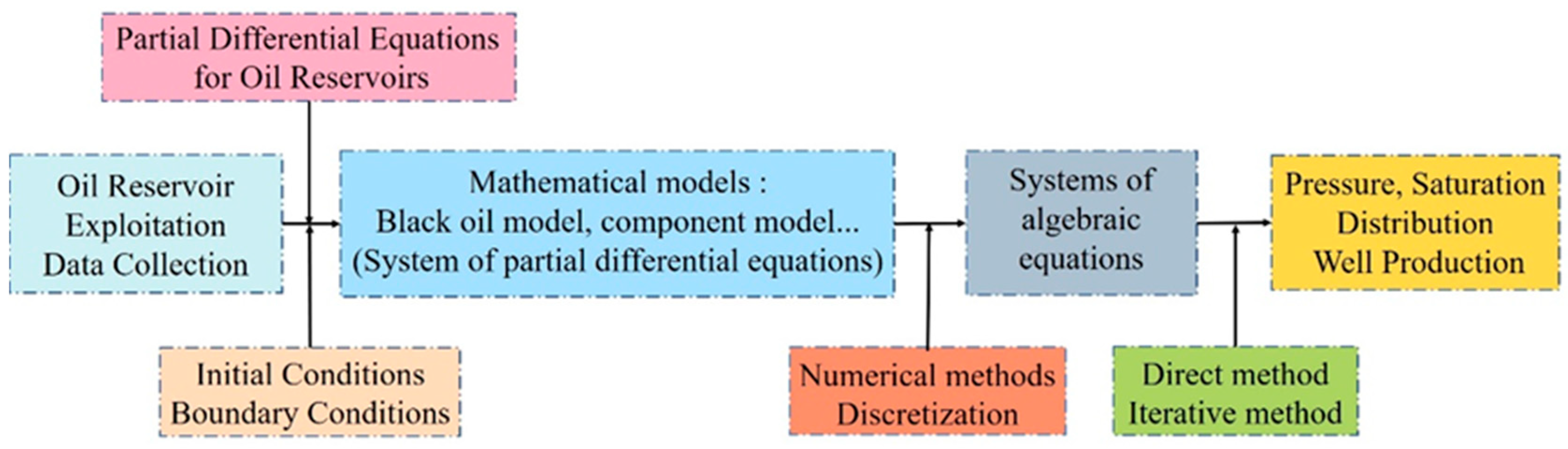
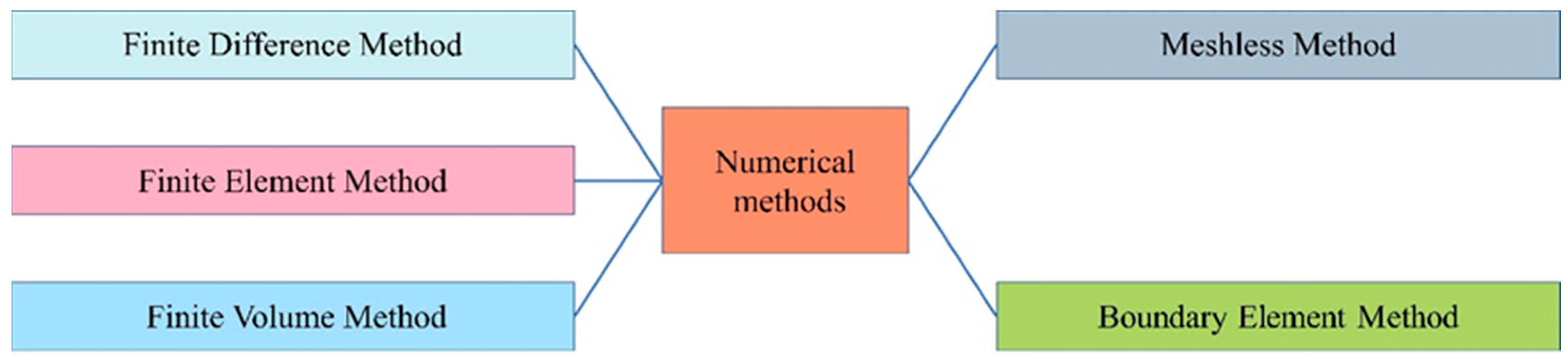
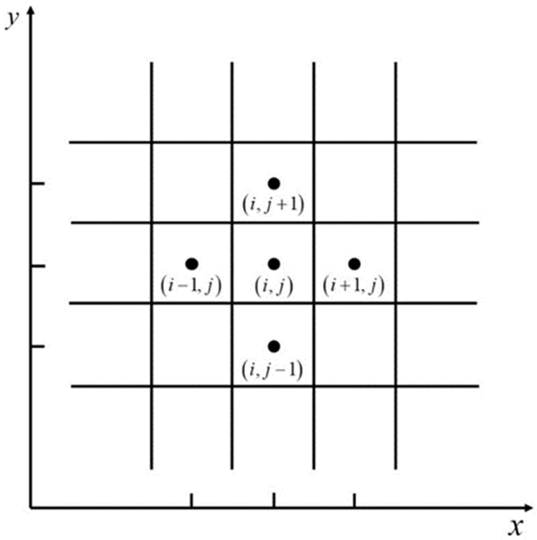
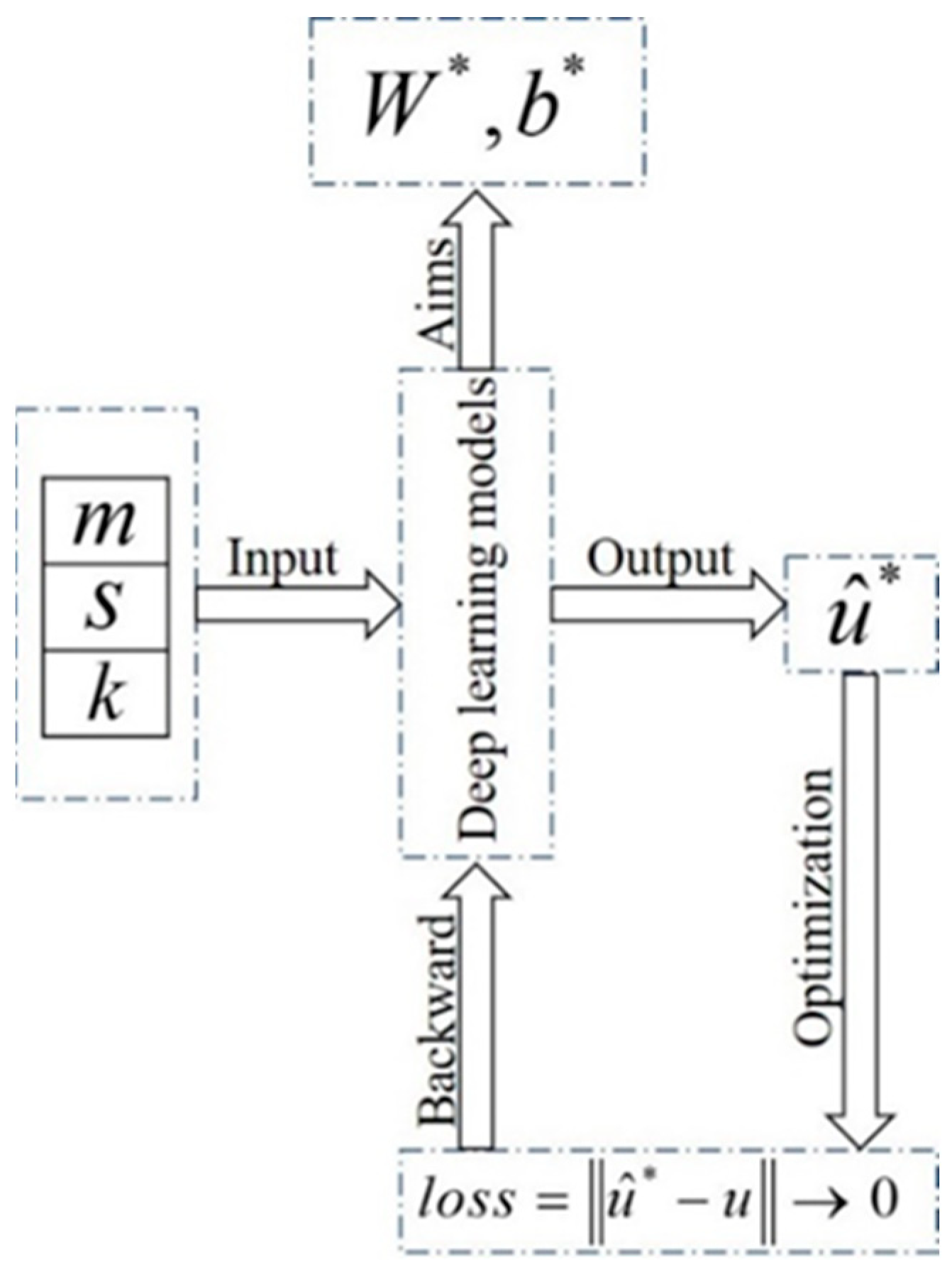
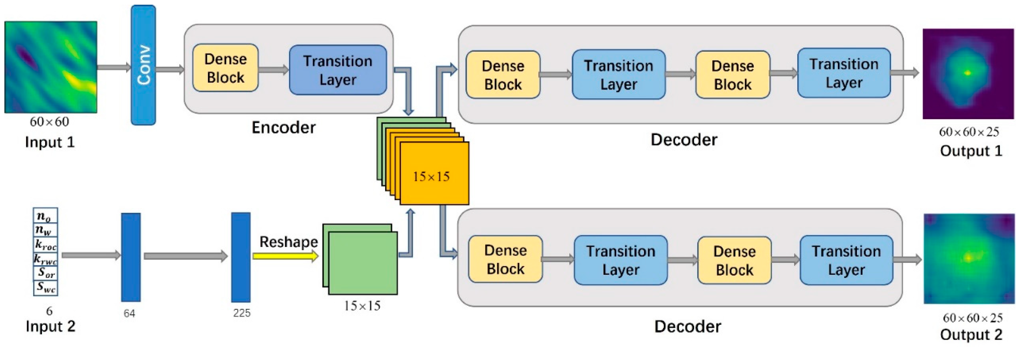
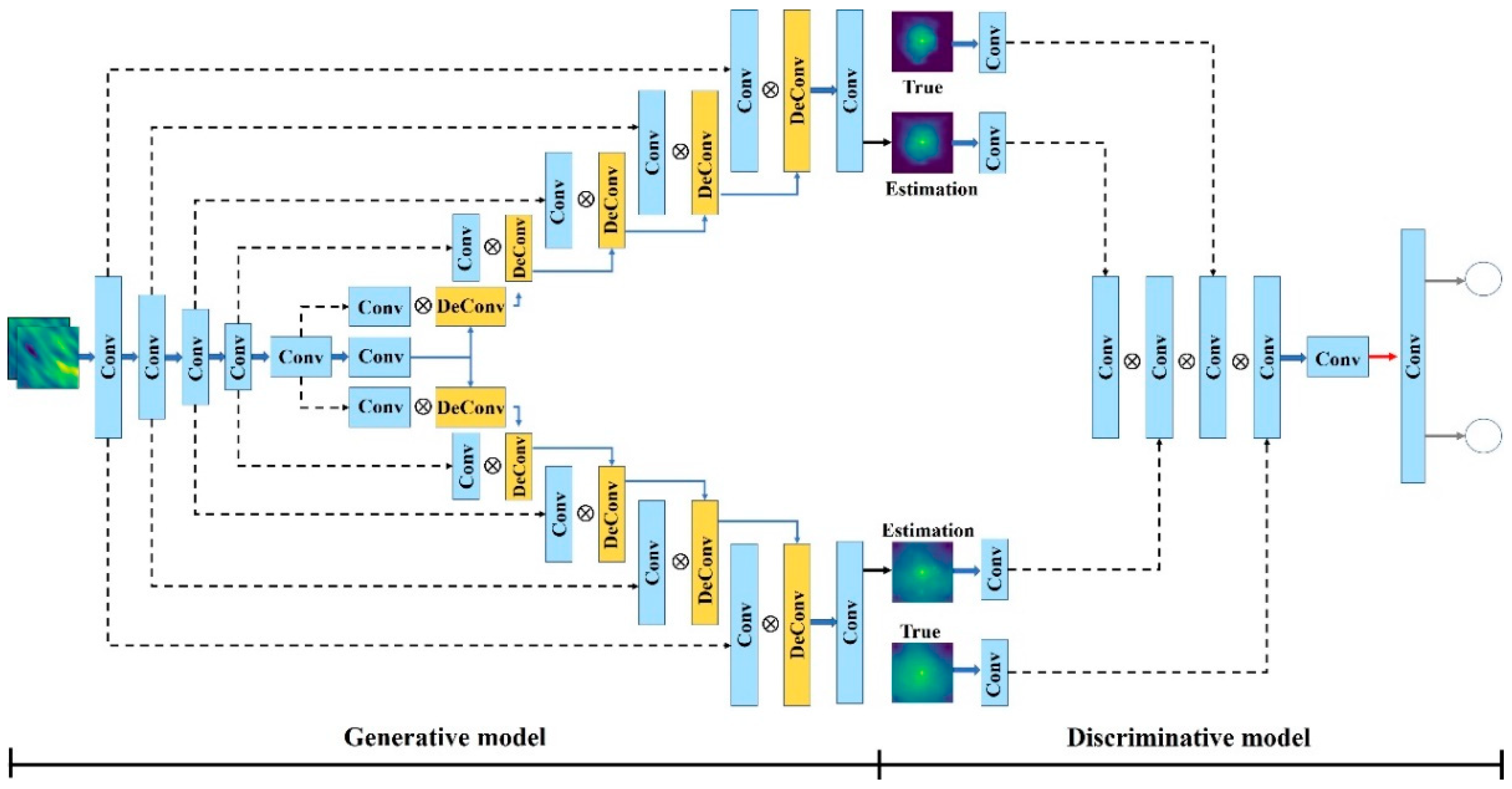
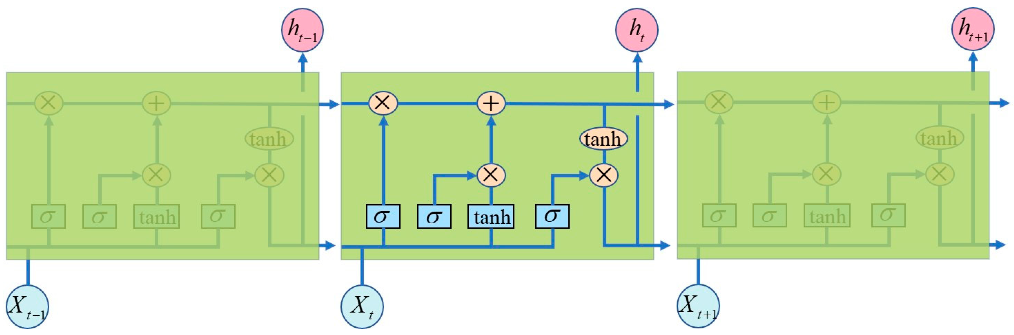
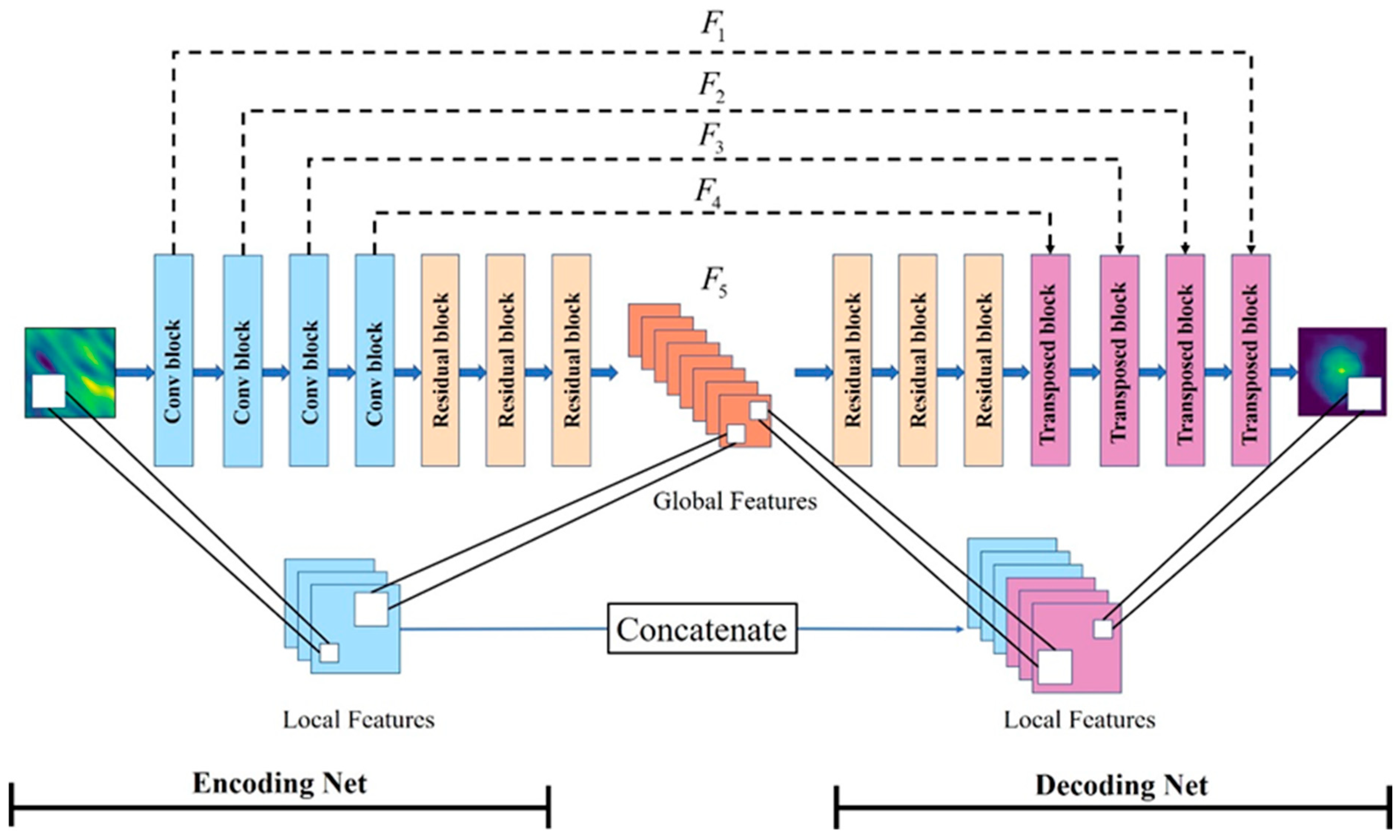
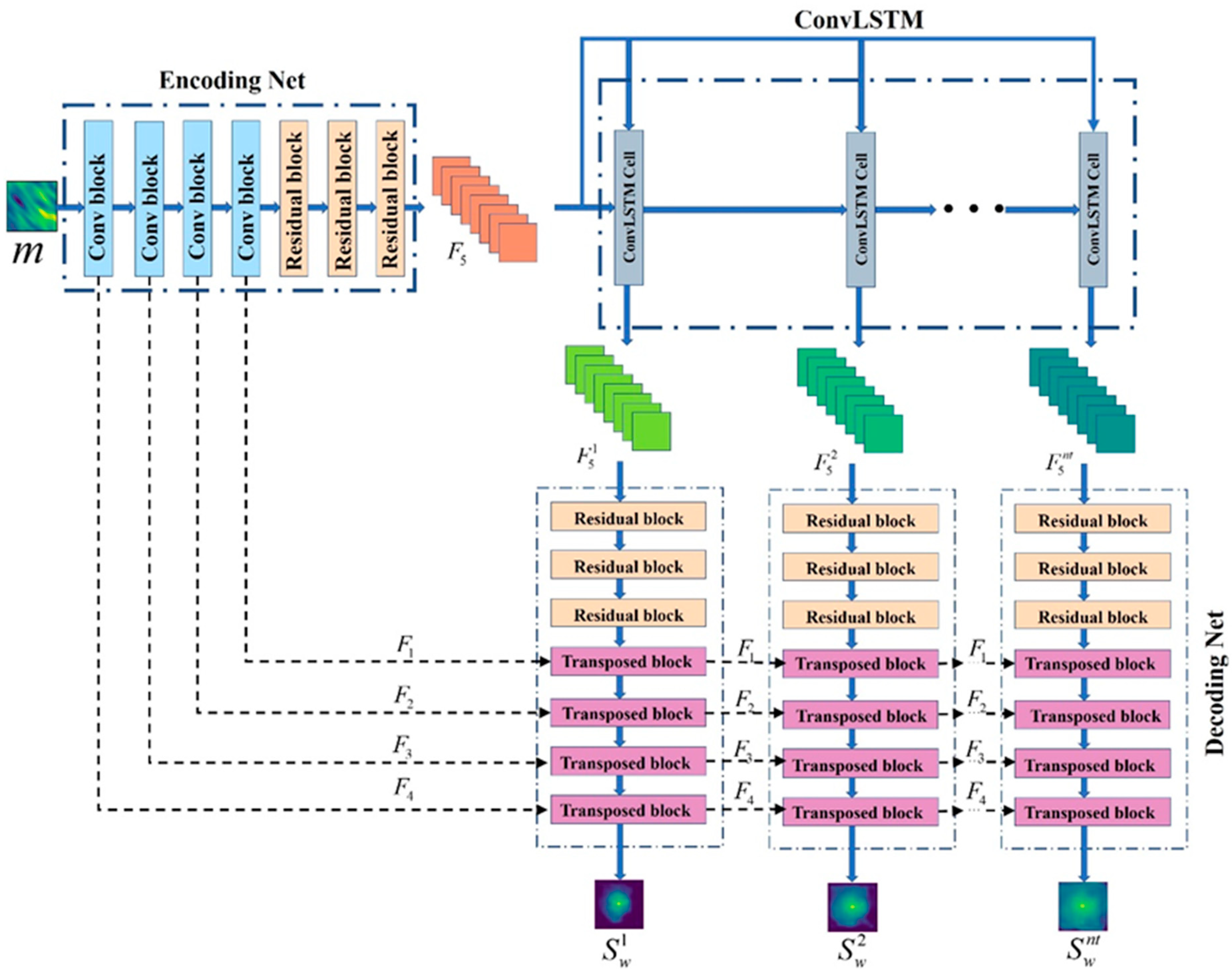
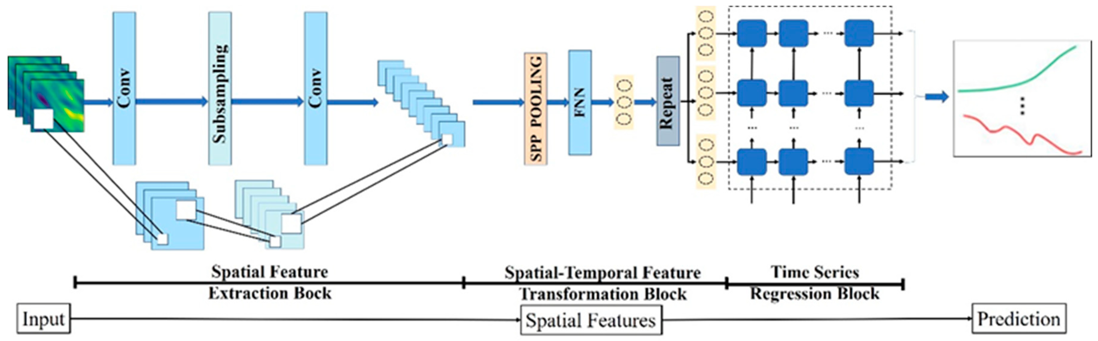
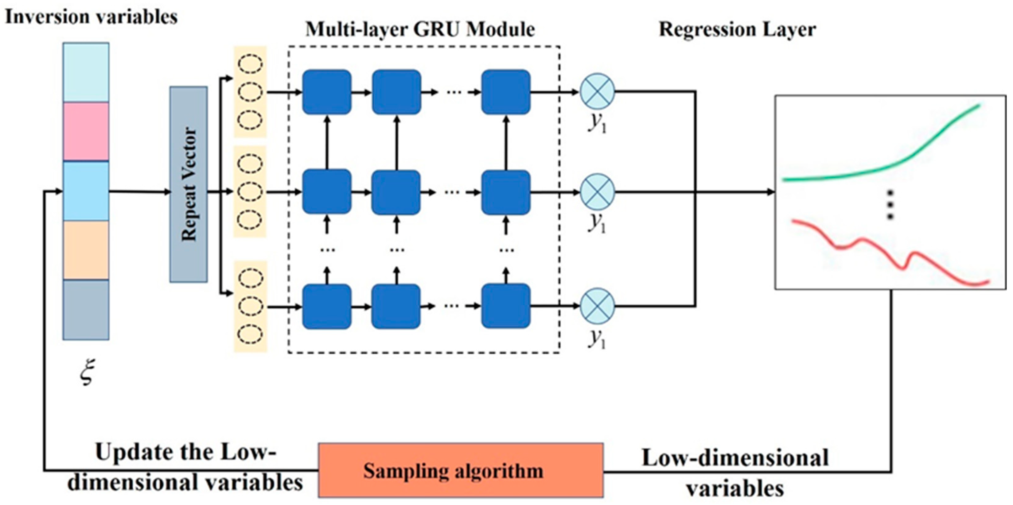
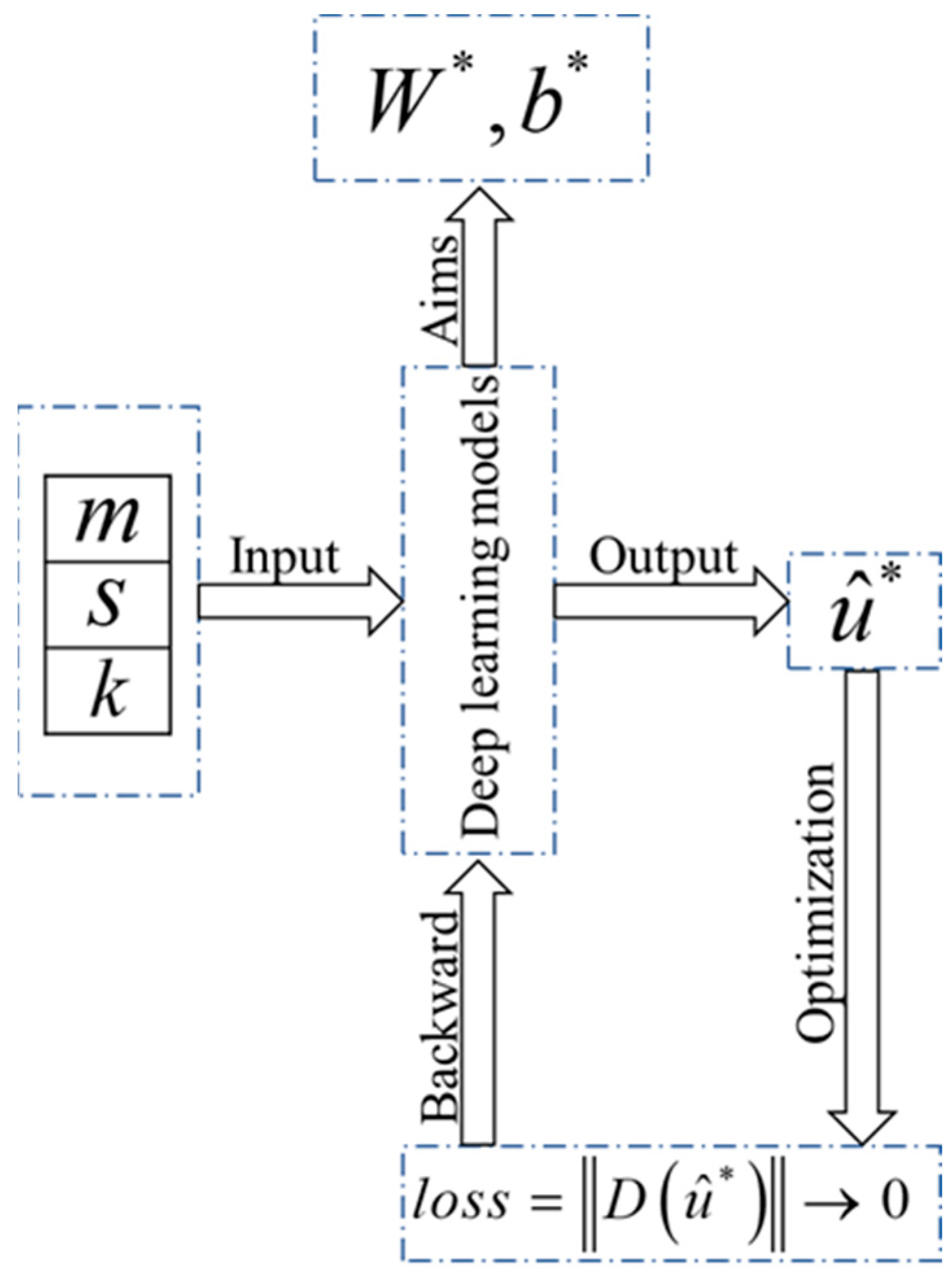
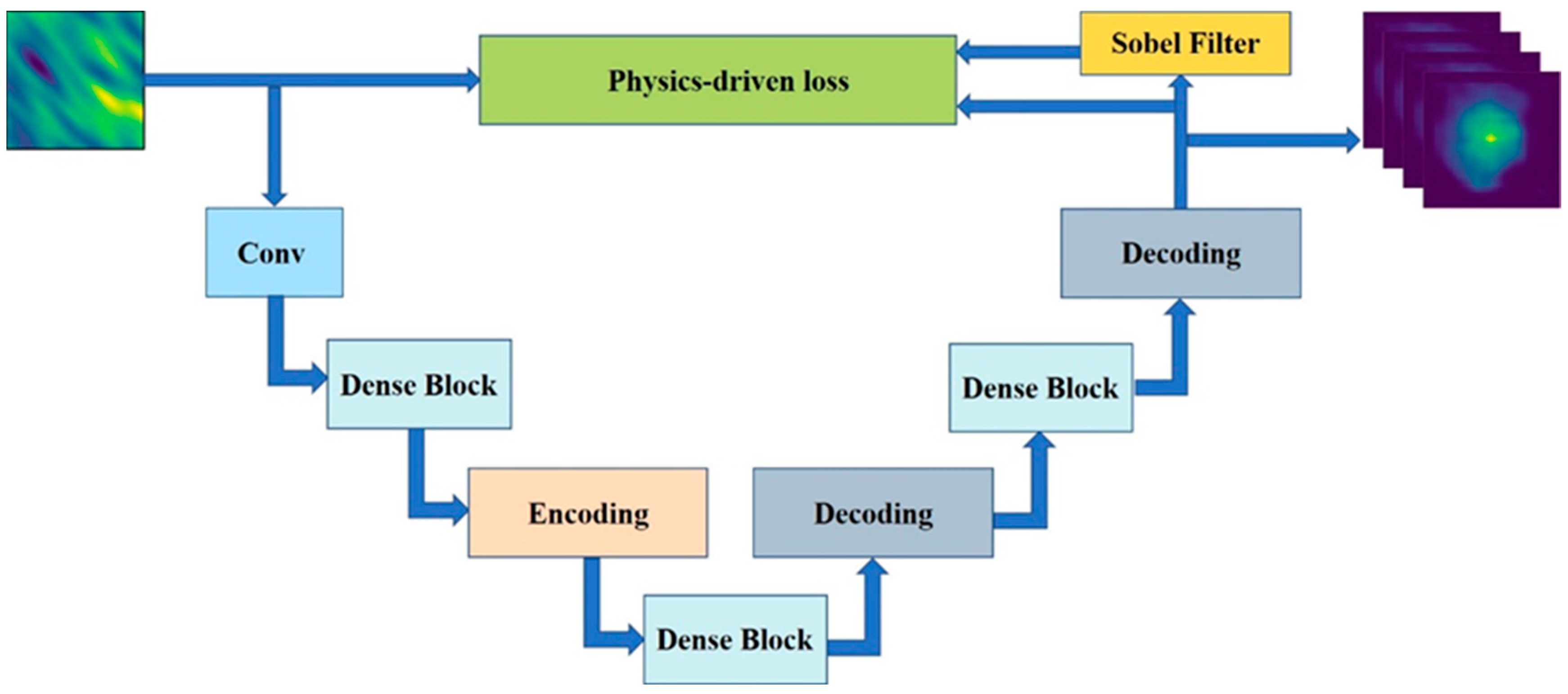
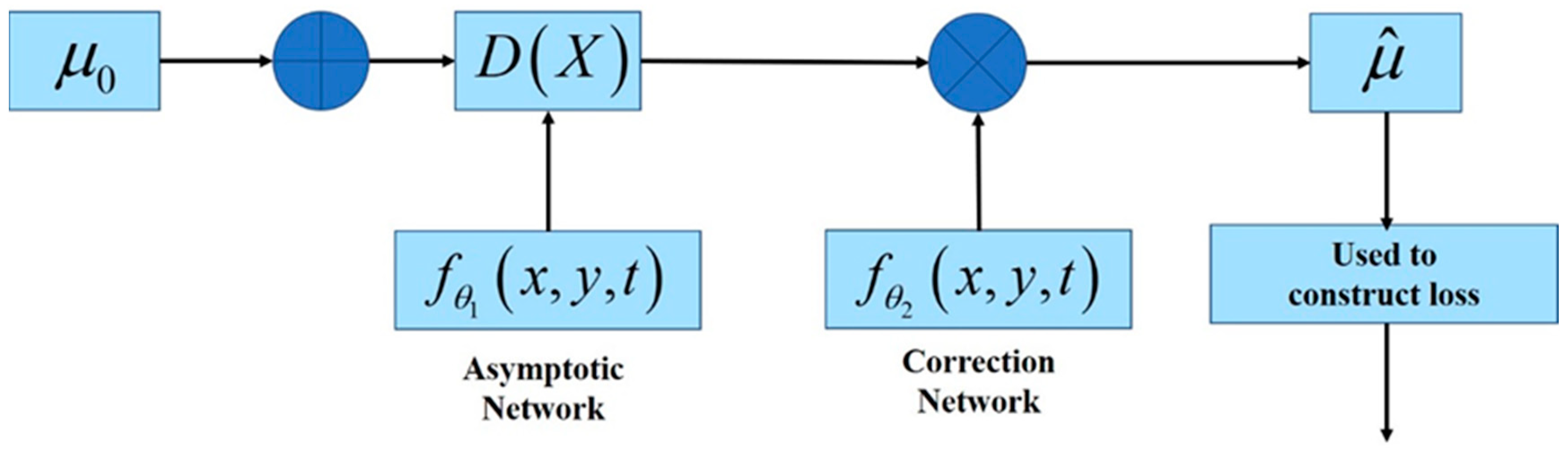
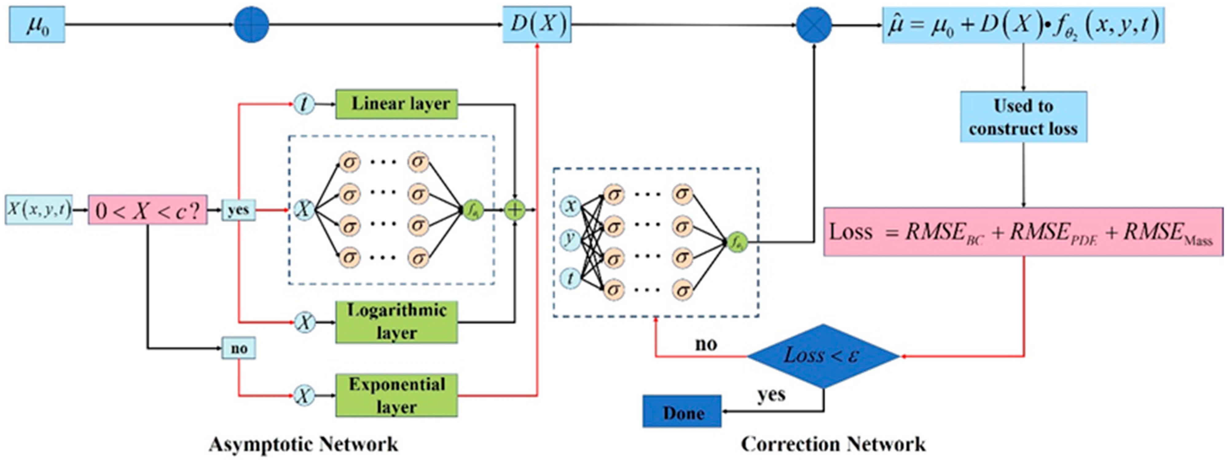
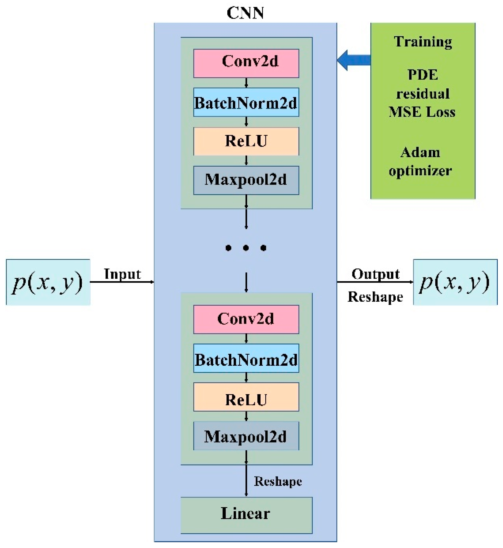
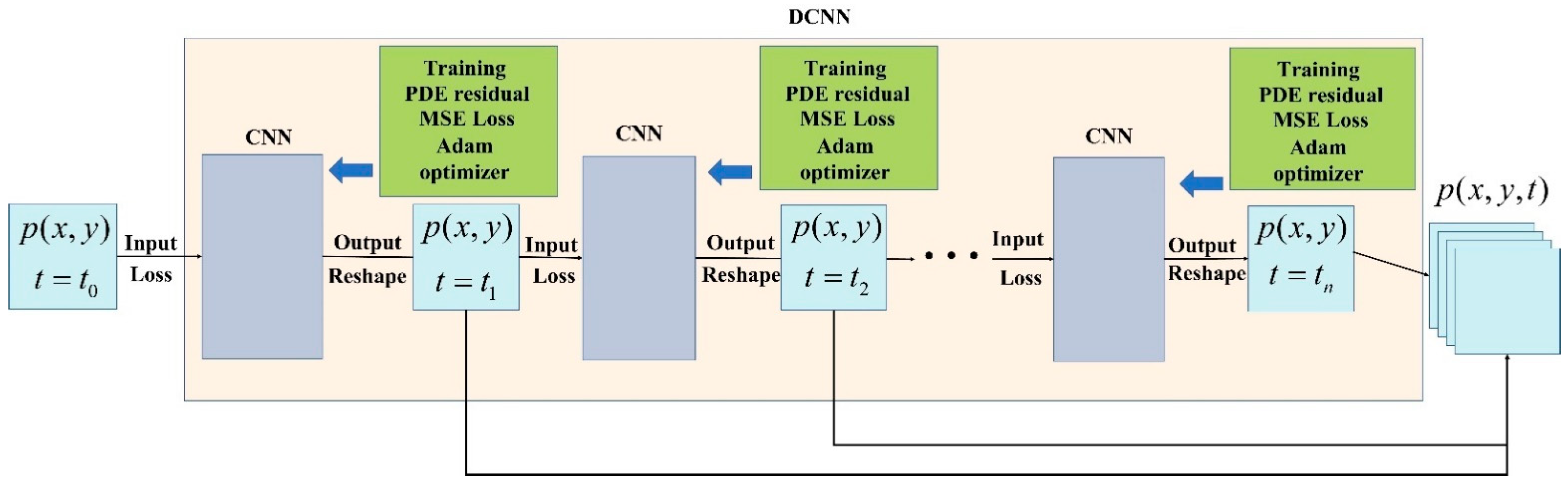
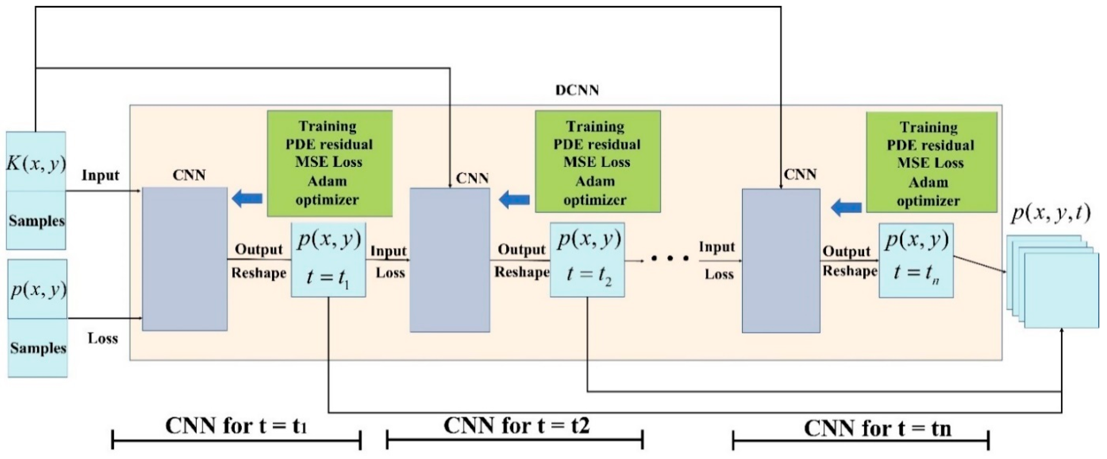
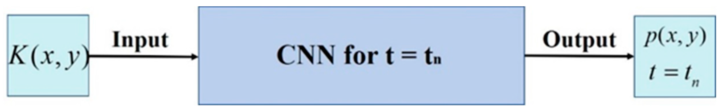
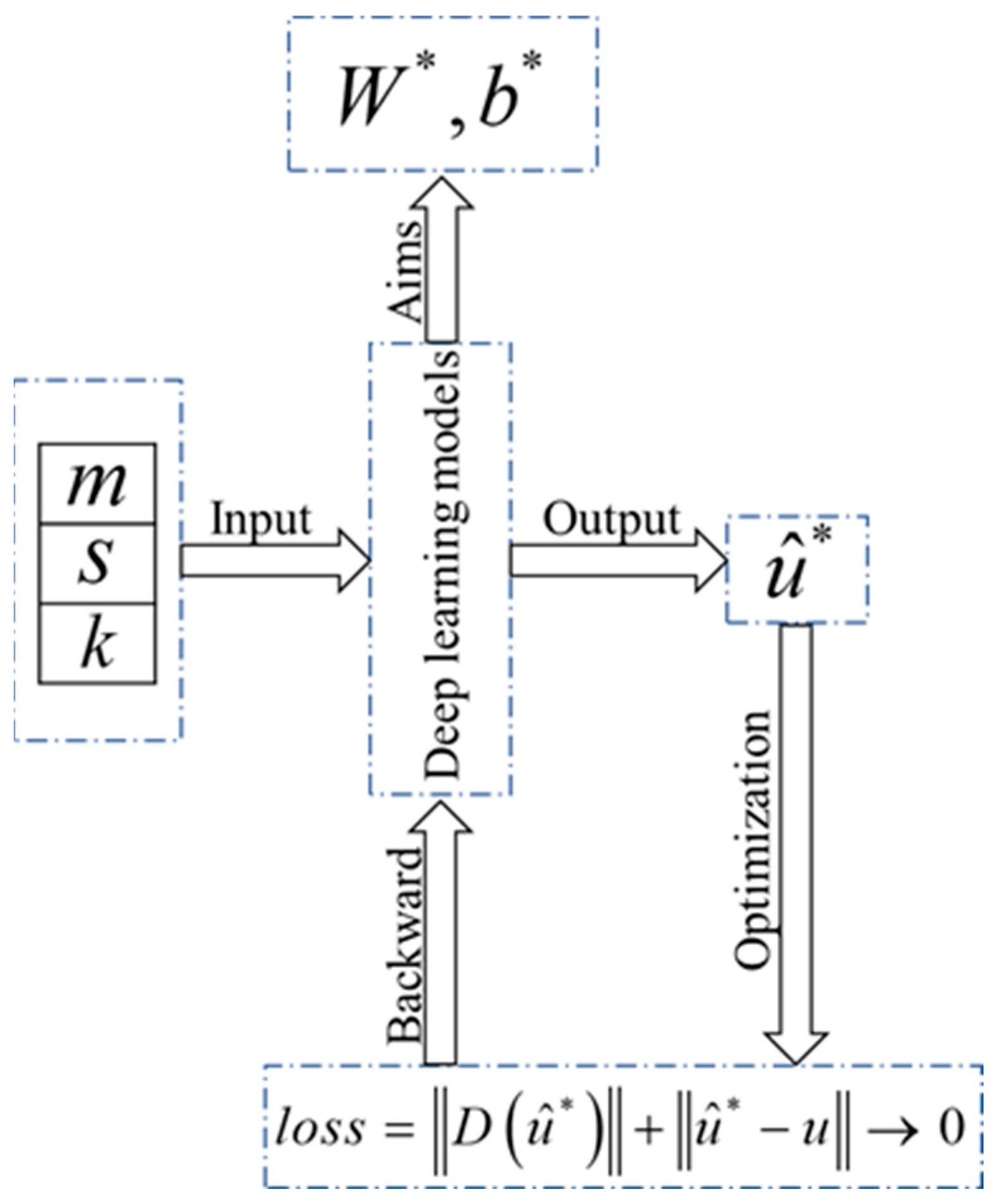
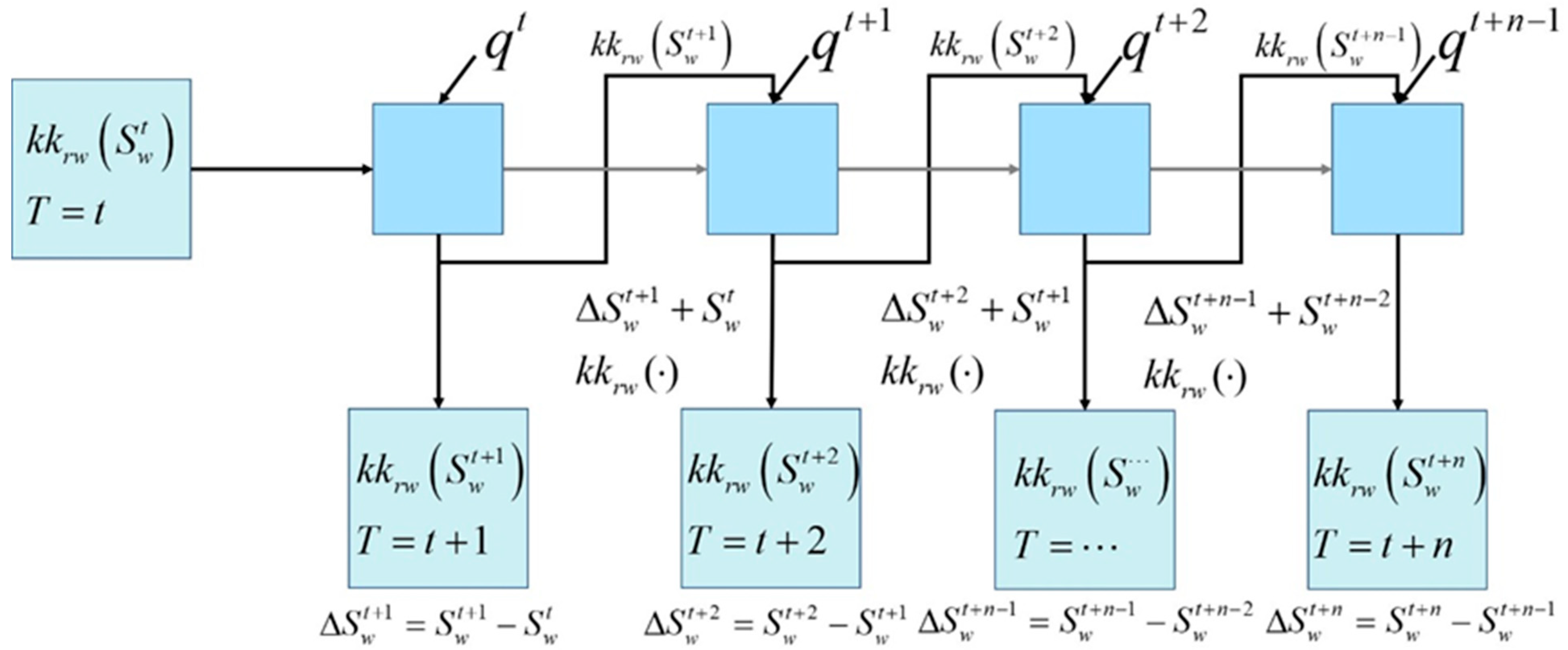
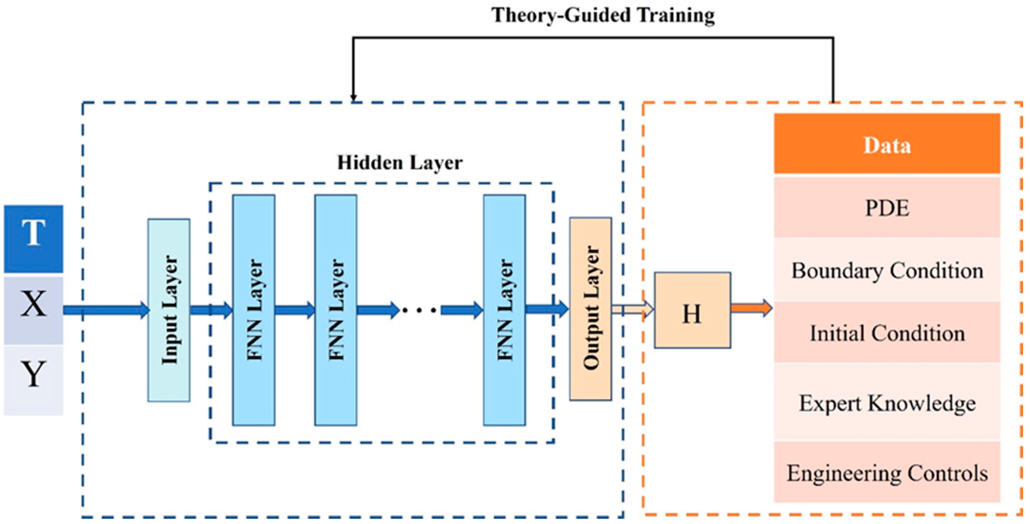
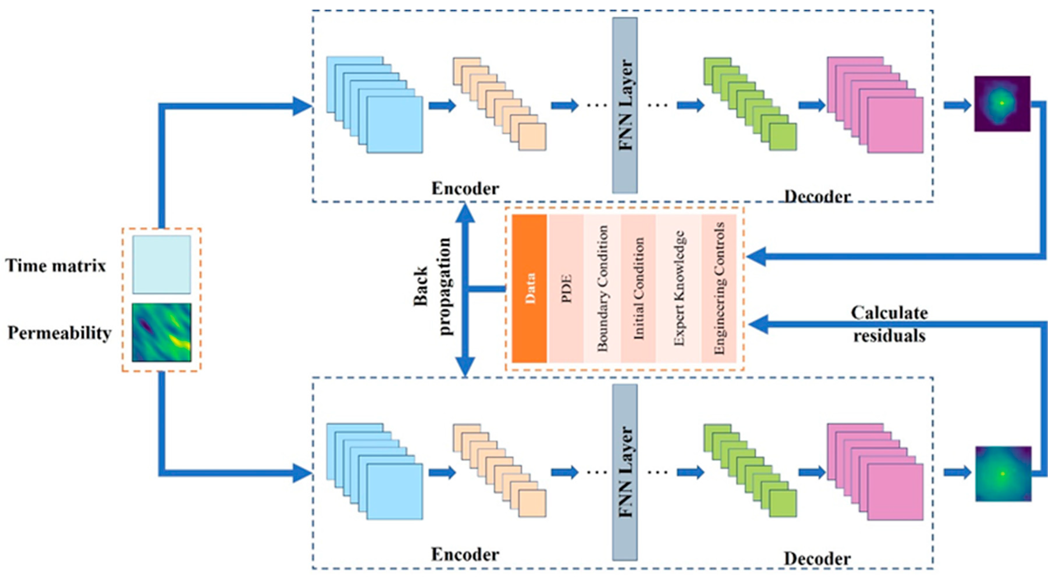
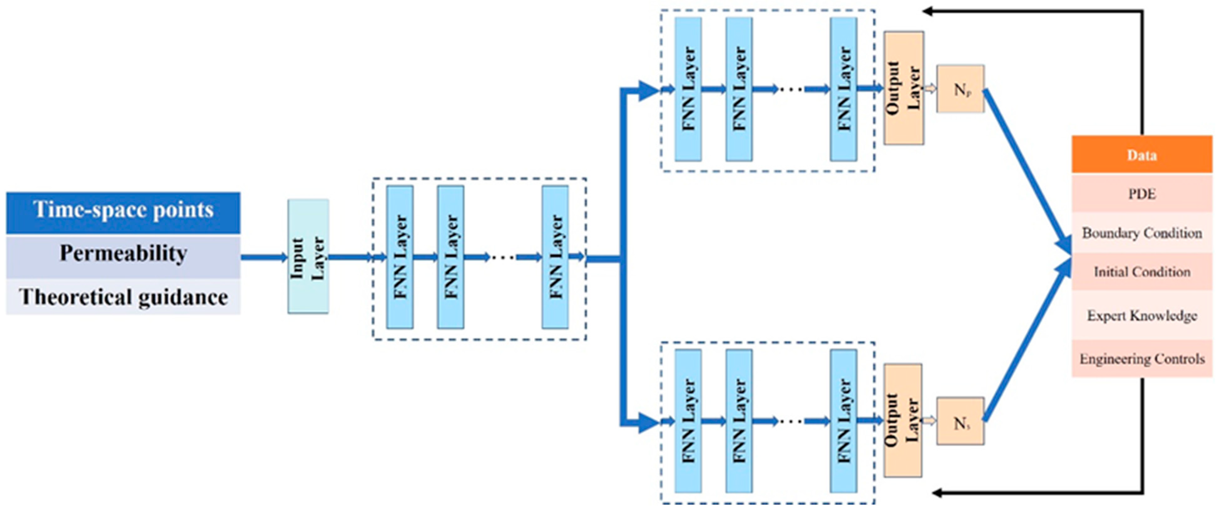6. Future Development and Prospects

Traditional numerical approaches, such as the finite difference and finite element methods, encounter challenges in certain intricate scenarios. Efforts have been made to bolster the efficacy of these conventional techniques by amalgamating the strengths of varied algorithms tailored to the distinct characteristics of reservoir models. Furthermore, by merging multiple traditional numerical strategies suitable for diverse scenarios, the robustness of these approaches is augmented. As these algorithms evolve, the foundational numerical methods will undoubtedly be enhanced.

Addressing the limitations inherent in conventional numerical methods, especially the computationally intensive phase equilibrium computations in component models, there has been a shift towards integrating machine learning techniques with these methods. This union capitalizes on the cost-effectiveness and efficiency of machine learning, aiming to expedite numerical simulation calculations, thereby facilitating swift and efficient reservoir simulations.

With the foray of deep learning techniques in petroleum engineering, the data-driven approach to solving partial differential equations has gained traction, chiefly due to its straightforward model architecture and broad applicability. However, a potential pitfall of this data-driven paradigm is its disregard for the physical laws governing the flow of oil and gas in porous media. This oversight can lead to skewed predictions that lack physical veracity. To rectify this, the physics-constrained approach to solving partial differential equations has emerged as a focal research area. This approach augments deep learning models by imposing constraints based on physical laws. Moreover, given the challenges associated with procuring field data and the models’ limited universality, physics-driven methodologies that solve reservoir partial differential equations without relying on labeled data are posited to dominate future reservoir intelligence research. As artificial intelligence continues its trajectory and computational capacities grow, the physics-driven approach to solving reservoir partial differential equations is poised to become a linchpin in the realization of the intelligent oilfield paradigm.