Particle Swarm Training of a Neural Network for the Lower Upper Bound Estimation of the Prediction Intervals of Time Series

Abstract

Many time series forecasting applications use ranges rather than point forecasts. Producing forecasts in the form of Prediction Intervals (PIs) is natural, since intervals are an important component of many mathematical models. The LUBE (Lower Upper Bound Estimation) method is aimed at finding ranges based on solving optimization problems taking into account interval width and coverage. Using the Particle Swarm Training of simple neural network, we look for a solution to the optimization problem of the Coverage Width-Based Criterion (CWC), which is the exponential convolution of conflicting criteria PICP (Prediction Interval Coverage Probability) and PINRW (Prediction Interval Normalized Root-mean-square Width). Based on the concept of the Pareto compromise, it is introduced as a Pareto front in the space of specified criteria. The Pareto compromise is constructed as a relationship between conflicting criteria based on the found solution to the optimization problem. The data under consideration are the financial time series of the MOEX closing prices. Our findings reveal that a relatively simple neural network, comprising eight neurons and their corresponding 26 parameters (weights of neuron connections and neuron signal biases), is sufficient to yield reliable PIs for the investigated financial time series. The novelty of our approach lies in the use of a simple network structure (containing fewer than 100 parameters) to construct PIs for a financial time series. Additionally, we offer an experimental construction of the Pareto frontier, formed by the PICP and PINRW criteria.

1. Introduction

The foundation of analytical forecasts are computed values, derived from predictive mathematical models. However, in many systems, there is a class of problems for which the most valuable are not the exact values of the predicted data, but reliable and trustworthy estimates of the range of their values [1,2,3,4,5]. For instance, in resource allocation planning tasks, the accuracy of the upper forecast boundary is crucial, and if the actual value exceeds the upper estimate, insufficient resources will be reserved, and the system will fail to function. Time series models, the forecast of which is constructed in the form of value boundaries, are called Prediction Intervals (PIs) [6]. The development of robust predictive interval models in information-analytical systems and decision-making systems is a relevant task with significant practical importance in modern big data processing systems [7,8,9,10,11].

Currently, PI-based methods are being developed that can provide specified requirements for time series forecast quality. One of the key methods is a non-parametric method for finding lower and upper PI estimates, which has been named LUBE (Lower Upper Bound Estimation) [12,13]. According to the LUBE method, a multi-criteria task is set with conflicting quality criteria, the compromise between which is determined by the Pareto set front, which is sought out via numerical methods [14].

Other approaches to obtaining intervals have also emerged: machine learning methods based on conditional quantiles [15,16], quantum regression forests [17,18], and gradients that increase regression. Neural networks are the most used methods [19,20,21] as they can have two outputs that represent the lower and upper bounds of the PIs. Models can be built to directly estimate the lower and upper boundaries of PIs, which can then be narrowed or expanded using optimization methods based on specified quality criteria, using the LUBE method [22,23,24], or by searching for a Pareto compromise [14,25].

The construction of a Pareto set is one of the approaches to solving multi-criteria tasks [26]. The Pareto principle involves searching for a set of non-improvable solutions under given quality criteria [27]. In other words, given two conflicting criteria, it is necessary to find such a relationship in the criterion space that improving the values of one quality indicator leads to a deterioration in another. The Pareto set can be referred to as a set of non-improvable solutions in the criterion space. An example could be a set of criteria (1) to minimize costs or (2) to increase some indicator. If criterion (1) were specified, the problem solution would be trivial as the minimum cost equals zero. But, this solution is unlikely to satisfy the researcher. However, this criterion is not meaningless. If we try to improve indicator (2), while minimizing costs, this is already a clearly meaningful task. It would be desirable to find such a dependency of criterion (2) on criterion (1), or in other words, some kind of formula (curve, dependency) that would allow us to determine how the quality of (2) depends on (1). This is the Pareto set. It would be good to know that at such-and-such costs we obtain benefit (2). Then, knowing this dependency, we can choose a compromise solution [28]. The Pareto set is a set of efficient compromises. Unfortunately, there are currently no methods for constructing the Pareto set in general form. But, we can construct an estimate of the Pareto set in the form of some front (Pareto front), which divides the feasible region in the criterion space into two areas: one where inefficient (improvable) solutions fall, and an area into which solutions cannot fall; the border of this area will be an estimate of the Pareto set. Since this is an estimate and may not take into account some individual points or even small areas, but still this front defines a compromise, it is proposed to be called the Pareto compromise.

We highlight two important works in the context of our article in this area. Publication [25] suggests dividing the entire training set into two parts and constructing a compromise as a CWC contradiction for two parts of the sample, and then evaluate the results using PICP and PINAW [29,30]. The work [14] presented a methodology for estimating Pareto optimal forecasting intervals using hypernets: POPI-HN. This method can estimate the full set of Pareto optimal solutions for the trade-off between PI coverage and width in regression problems.

However, the proper selection of criteria could allow quite a simple ANN model to be efficient in the task of Prediction Interval construction following the LUBE approach.

Thus, in this paper, we will develop an algorithm for searching for interval solutions with boundaries constructed using the LUBE method, which represents a compromise under conditions of conflicting criteria. As an example, we will consider a financial time series, which will allow readers to independently replicate and interpret the results of this paper. We present a notebook as a Supplemental File that will allow you to repeat or modify our calculations. The contribution of this paper is as follows:

(1)

For the forecast interval, the LUBE problem with specified conflicting criteria is considered.

(2)

Using the Particle Swarm Training of a simple neural network, we look for a solution to the optimization problem of the CWC, which is the exponential convolution of the PICP and PINRW.

(3)

The concept of the Pareto compromise is introduced as a Pareto front in the space of specified criteria. The Pareto compromise is constructed as a relationship between PICP and PINRW based on the found solution to the optimization problem.

The subsequent organization of the article is as follows—Section 2 describes the materials and methods, Section 3 is devoted to the algorithms and parameters of machine learning, Section 4 presents the results, Section 5 is the discussion, and Section 6 is the conclusion.

2. Materials and Methods

A detailed formal formulation of the problem is given in [31,32].

The essence of the task is as follows. Let there be a given time series T. Based on historical values, it is necessary to forecast the ranges of future values of this time series T. For the given confidence level (CL) of prediction, a random Prediction Interval (PI) may be built based on previous observations; such PIs will enclose a future observation within a specified range with the probability equal to the CL. Let l and u be the lower and the upper bound of a PI correspondingly with CL = (1 − α)%, then the future unknown observation y_t+1 of the predicted variable Y will belong to the PI = [l; u] with the probability (1 − α). Thus, PIs provide the information about the accuracy of prediction, unlike deterministic forecasts. The prediction accuracy information in its turn is essential for risk assessment, decision making, and planning. For a given CL, narrower PIs should be preferred as they clearly contain less uncertainty and deliver more information to the analyst. The modern wide application of artificial neural networks (ANNs) allows one to build complex non-linear tools for interval forecasting relatively easily.

Among other techniques, the Lower Upper Bound Estimation (LUBE) technique stands out for its efficiency and straightforwardness in the task of constructing high precision PIs with ANNs. It was shown previously [12,13] that LUBE outperforms classic PI construction methods such as Bayesian methods, the delta method, and bootstrapping.

Let us build a LUBE solution by compiling an ANN with two output neurons for the direct approximation of the lower and upper bounds of the interval (Figure 1).

Such a structure of the ANN implies that the interval between the two outputs would contain each actual value of the predicted variable with the probability of (1 − α). The ANN is trained using previous observations of the predicted variable as well as, optionally, some other relevant inputs. In this paper, we focus on a single-input LUBE ANN.

To train the ANN, a proper loss function (criterion) should be selected. As we discussed previously, our goal is to obtain narrower intervals which contain a true value with the certain probability. To address this problem, a couple of intuitive criteria were proposed in the literature. The first one is Prediction Interval Coverage Probability (PICP) and the second one is the Prediction Interval Normalized Root-mean-square Width (PINRW):

$$\mathrm{PICP}=\frac{1}{n}{\displaystyle \sum }_{i=1}^n{c}_i,$$

(1)

where n is the number of observations, $c_i$ is equal to one of the observations $y_i\in \left[l_i, u_i\right]$ and zero; otherwise,

$$\mathrm{PINRW}=\frac{1}{R}\sqrt{\frac{1}{n}{\displaystyle \sum }_{i=1}^n{\left(u_i-l_i\right)}^2},$$

(2)

where R is the range of the observed variable.

Thus, the greater PICP corresponds to the greater percentage of actual observations which fitted into the predicted bounds, while the lower PINRW would lead to narrower intervals. Therefore, in ANN training, our goal is:

$$\{\begin{array}{c}\mathrm{PICP} \underset{}{\to }max\\ \mathrm{PINRW} \underset{}{\to } min \end{array}.$$

(3)

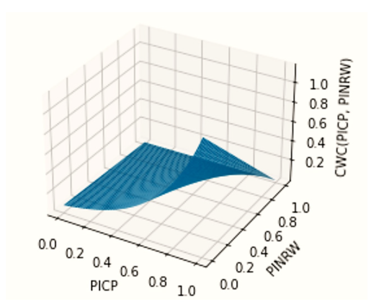
As a single function is often used as the loss during ANN training, we decided to choose the normalized Coverage Width-Based Criterion (CWC) as a non-linear convolution of the PICP and PINRW:

$$\begin{gathered} \mathrm{CWC} =\left(1-\mathrm{PINRW}\right)e^{\eta \left(\mathrm{PICP}-\mu \right)}; \\ \mathrm{CWC}\underset{}{\to }max, \\ \mathrm{PICP} \subseteq \left[0;1\right] \end{gathered}$$

(4)

where $\mu$ is set to (1 − α), while $\eta$ defines the slope of the CWC surface.

Figure 2 presents an example of a CWC surface for $\mu =0.95, \eta =3$. It can be observed that the CWC function, being a functional combination of conflicting criteria (maximizing the number of points falling within an interval and minimizing the width of the interval), represents a compromise dependence expressed in the form of Equation (4). In other words, the CWC defines how much one can sacrifice the width of the interval in order to accommodate as many points as possible. It should be noted that there is a certain level in this task that is uncharacteristic for multi-criteria tasks, i.e., there exists a sufficiently large width of the interval that will assuredly encompass all points, and this interval value is finite (less than infinity). A specific issue with the CWC is that the function defined as Equation (4) is highly non-linear and complex, rendering the application of fast gradient back-propagation techniques irrelevant.

It should be noted that, instead of a CWC, quality-driven (QD) differentiable criteria could be applied as in work [14]. However, a CWC is more widely used, while QD differentiable criteria demand large batch sizes (50 points and more) for the training to be sustainable, as they utilize the central limit theorem to approximate the binomial distribution during the derivation, which is not often appropriate for various tasks of time series prediction, and should be further studied.

Although a linear convolution may be a compromise, both in the case of the CWC and in linear convolution, there is an assumption about the form of dependence of the criteria, which is expressed in the hypothesis about the computability of the coefficients, which, in practice, cannot be reliably and justifiably calculated. Without additional hypotheses about the form of dependence, the application of the Pareto principle is appropriate. In this case, a functional dependence of one criterion on another is constructed, and the compromise is represented by the depicted dependence.

We aim to define a numerical assessment of the Pareto set within the criteria space as a numerical appraisal of the boundary delineating the set of feasible solutions from the set of enhanced solutions. This definition aligns with Pareto’s conceptualization of the set of solutions that cannot be further improved. Given that this boundary is numerically determined rather than analytically determined, we refer to the resultant front as a Pareto compromise.

The theoretical solution for finding the Pareto compromise can be found from the following considerations. From (1), it can be seen that the PICP tends to 1. That is, starting from a certain interval value, all points will fall within the interval, i.e., PICP = 1 (Figure 3).

For the purpose of finding this Pareto compromise, we propose using the Particle Swarm Optimization (PSO) algorithm, as gradient descent methods are not suitable for optimizing a CWC.

It should be noted that the slope of the frontier on Figure 3 is dependent on the nature of the data being studied and for each task will be determined experimentally during the construction of the Pareto compromise through the selection of parameters for the LUBE neural network with PSO and the calculation of corresponding PINRW and PICP values when computing a CWC. The experimentally constructed Pareto frontier for our task is presented in Section 4 (Figure 4).

3. Algorithm and its Implementation

The algorithm begins with the setup of necessary modules and libraries (PySwarms, Tensorflow, and others). Then, time series data are loaded. After this, the data are normalized within the range (0, 1) and divided into a training and validation set in an 80/20 ratio. Then, CWC surface exploration and $\mu , \eta$ parameter selection is conducted. The programming of Formulas (1), (2), and (4) is carried out in the form of Python functions.

An ANN model was defined using the Tensorflow Sequential API. The ANN consisted of three dense layers with 3, 3, and 2 neurons each from input to output (Figure 4). Linear activation was used to transmit the signals between the layers. The ANN had a total of 26 parameters (Figure 5).

The reason we chose this particular neural network structure is due to its simplicity and sufficiency for modeling the time series of the MOEX closing prices that we are studying. To find such a structure, we sequentially conducted experiments by increasing the number of neurons, starting with a two-layer network with one neuron at the input and two neurons at the output (as required by the LUBE method).

It should be noted that, as the number of neurons in the network increases, so does the dimensionality of its parameter space (weights of connections and biases of neuron signals). In the neural network structure we are considering, there are 26 parameters, which allows us to directly apply PSO for finding the optimal set of parameters (i.e., for training the network) on a standard personal computer equipped with an Intel Core i7 processor and 12 GB RAM, while such a network is capable of successfully predicting the time series under consideration.

However, of course, more complex networks can also be used, including recurrent ones such as the LSTM for analyzing data for which simple networks (containing less than 100 parameters) proved to be insufficient. In this case, the question arises of obtaining an initial approximation of network parameters for directing the PSO algorithm and the possibility of obtaining a solution within an acceptable time on a personal computer.

One of the ways to obtain an initial approximation that we have tried is to use a differentiable loss function, for example, MAE, in the task of predicting a point value of a series, rather than an interval. In this case, the outputs of the neural network are equal to each other and correspond to the value of the point forecast.

Starting from weights and biases found in this way, it is possible to obtain a solution using PSO within an acceptable time for the task of PI construction based on the same data used for the initial approximation.

For simple networks with less than 100 parameters, it is possible to apply PSO directly and there is no need for sophisticated methods of initial approximation derivation to reduce the duration of the PSO search.

To train the ANN, a normalized CWC function (4) was chosen as a basis to calculate the cost for a PSO algorithm implemented with pyswarms library. As the library algorithm is aimed at the minimization of the cost function, the function 1−CWC was used as the cost to ensure the maximization of the CWC and to solve task (4). The following parameters were used for the CWC: $\mu =0.95, \eta =3$.

The Particle Swarm Optimization (PSO) algorithm is chosen to select the weights of the ANN because it is proven to be able to find nearly optimal solutions in non-linear context [33]. PSO belongs to the population-based search methods inspired by natural processes such as bird flocking and fish schooling [34]. The positions of the particles during the search represent the vectors of candidate solutions to the problem being optimized. In the case of LUBE ANN training, each particle position represents the weights and biases of the ANN. After the weights and biases are applied, the prediction is performed with the ANN and the 1−CWC value is computed and recognized as the cost of the candidate solution. After evaluating all the particle costs, the positions are adjusted in the direction of the best solution and the next iteration of cost evaluations is performed.

The boundaries for the coordinates of swarm positions (i.e., weights and biases of perceptron) were set to [−1.0; 1.0] for each coordinate as the data were normalized.

Other PSO parameters were chosen as follows:

• Number of particles: 30;
• Dimensions: 26;
• Learning factor c₁: 0.5;
• Learning factor c₂: 0.3;
• Inertia weight w: 0.9;
• Number of iterations: 1000.

It should be noted that the swarm of particles does not guarantee that a good solution is found and transferred from iteration to iteration and improved by default. It is quite possible to deteriorate previously found solutions if the appropriate parameter of the library is not set and the best position is not kept. In this case, it is necessary to evaluate the entire pool of solutions obtained throughout all iterations of the algorithm, not just the sample of the last iteration. One should also be careful with selection learning and the inertia weight factors of the algorithm. If you increase the learning factor recklessly, it can cause the particles to move too fast, potentially causing them to overshoot the optimal solution. This could lead to oscillation around the optimum or even diverge, resulting in a failure to converge to the best solution.

Inertia weight is a parameter in PSO that controls the influence of a particle’s previous velocity on its current one. It helps balance the global and local exploration abilities of the swarm, allowing for both the exploitation of known good regions and the exploration of new ones. A high inertia weight encourages more global exploration (jumping to new areas), while a low inertia weight encourages more local exploration (fine-tuning within a current area).

As for adjustments, there are different strategies. One common approach is to gradually decrease the inertia weight over time, starting from a higher value for more global exploration in the beginning and then lowering it to allow for more local fine-tuning as the algorithm progresses. The learning factors can also be tuned during the run, but it is important to maintain a balance between them to ensure that neither personal bests nor global bests dominate the updating process.

It was also noted that the genetic algorithm (GA) can sometimes converge faster than PSO due to its inherent diversity and robustness. The GA uses operations such as crossover, mutation, and selection that mimic natural evolution, which can help it explore a broader search space and potentially find good solutions more quickly.

However, this same characteristic can also lead the GA to become stuck in local minima more often than PSO. This is because, while the diversity of solutions in the GA can help it jump out of local minima, the randomness in the selection, crossover, and mutation processes can also cause it to lose good solutions and become trapped.

To achieve similar results with the GA as with PSO, there are several strategies to be adopted. One is to use elitism, where the best individuals from each generation are guaranteed to carry over to the next. This can help maintain good solutions and prevent them from being lost due to the randomness of GA operations.

Another strategy is to adjust the rates of crossover and mutation. A high crossover rate can encourage the exploration of new areas in the search space, while a high mutation rate can help maintain diversity and prevent premature convergence. However, these rates should not be too high, as excessive crossover or mutation can disrupt good solutions and lead to instability.

Finally, hybridizing the GA with other optimization techniques, such as PSO, could also be an effective way to balance exploration and exploitation. This can combine the strengths of both algorithms: the robustness and diversity of the GA, and the ability of PSO to fine-tune solutions and avoid local minima. The investigation of such hybridization will be the next stage of our studies.

4. Results

The Moscow Exchange (MOEX) is the largest exchange in Russia, operating trading markets in equities, bonds, derivatives, the foreign exchange market, money markets, and precious metals. To forecast the intervals, the closing prices from the MOEX were selected from 3 March 2003 to 29 March 2023. The training set consisted of the first 80% of data from the start until 15 March 2019. In total, there were 4007 data points in the training set and 1001 data points in the test set. The data were normalized in the range [0; 1].

After 1000 iterations of swarm search, the best ANN parameters were identified with a cost of 0.0983 and corresponding CWC value of 0.9017.

To investigate the surroundings of the best solution more precisely, the learning factors c₁ and c₂ were reduced to 0.05 and 0.03, respectively, and the inertia weight w was reduced to 0.1. The number of particles was reduced to 3. After a further, much faster, 1000 iterations, the best cost was reduced to 0.0653 and the corresponding CWC value increased to 0.9347. The resulting prediction plot on the test data is depicted in Figure 6.

The vector of model weights for the final solution was as follows:

[0.17669555 −0.58701599 0.72388002 0.42600467 −0.02259329 0.00271661 0.23010153 0.04476818 0.1479215 0.81946032 0.50182296 −0.5798633 −0.74183443 −0.07945618 0.44274501 0.37159384 −0.24637542 0.47058104 −0.64647528 −0.82920599 0.04508022 −0.15889919 0.65014887 0.1793743 −0.11517166 0.26014331]

If what is needed is not a solution, but a compromise, which makes it possible to operate with the ratio of the PINRW and PICP criteria when making a decision, then a Pareto front can be constructed in the space of criteria. A Pareto compromise can be constructed for the final solution to the CWC optimization problem. Figure 7 shows the distribution of solutions during the PSO search according to their PICP and PINRW values. It should be noted that, due to the contradiction of the PICP and PINRW criteria, some other solutions on the boundary of the Pareto front could be selected depending on the goals of the modeling.

Figure 7 illustrates the distribution of solutions (sets of LUBE-neural network parameters) over the course of 1000 iterations of particle swarm search, relative to the corresponding PINRW and PICP values for each solution (each point). We observe that the solutions explored by the swarm are located in the right region of the graph, where a distinct (green) front of non-improvable solutions can be clearly identified, forming the Pareto compromise boundary we theoretically estimated (Figure 3). Thus, the blue points correspond to dominated solutions, for each of which there exists a non-improvable (green) solution on the Pareto front boundary.

5. Discussion

In the process of parameter selection (training) for neural networks, gradient and gradient-free methods are distinguished. On the one hand, the progress in the field of deep learning in recent years is largely owed to gradient training methods. On the other hand, gradient solvers can become stuck in a local minimum and there are isolated examples of tasks, such as the optimization of a CWC, where the use of a gradient solver is either impossible or the training process is not stable. There is also a debate as to whether the gradient model for training neural networks is suitable for multi-criteria tasks at all. Due to the fact that the PICP often does not produce a gradient, it is practically impossible to apply the gradient learning methods of the neural network for searching for weights of connections and neuron biases.

A limitation of our approach is the non-linear convolution of conflicting PICP and PINRW criteria, defined in form (4), which is used as a loss function for the Lower Upper Bound Estimation (LUBE) neural network.

The quality-driven differentiable criterion proposed by [9] in 2018 to replace the CWC is based on several assumptions: the PICP values for different points are independent and they follow a Bernoulli distribution. Pearce et al. [9] himself points out that this assumption may not hold for data points that are too close to each other, and yet “we believe holds sufficiently for a randomly sampled subset of all data points” [9]. This assumption allows all data points to be considered as following a binomial distribution. The central limit theorem (Moivre–Laplace theorem) is then used to approximate this binomial distribution for a larger number of data points. This leads to the conclusion that a batch of data should contain no less than 50 points, which significantly limits the application of the method in some time series analysis tasks.

On the other hand, as demonstrated in our paper, direct use of the CWC and population-based gradient-free training methods is quite possible, and relatively small networks with a small number of parameters (<100) can handle the prediction of upper and lower boundaries of stochastic non-stationary time series intervals.

6. Conclusions

This article develops a method for obtaining a decision on the selection of PI boundaries based on CWC optimization using a neural network and Particle Swarm Training.

We demonstrated the application of a simple network structure, consisting of less than 100 parameters, in constructing Prediction Intervals (PIs) for a financial time series. Furthermore, we conducted an experimental construction of the Pareto frontier, shaped by the Prediction Interval Coverage Probability (PICP) and Prediction Interval Normalized Average Width (PINRW) criteria.

The future of this research is the use of alternative algorithms for searching network parameters, such as Particle Swarm Optimization (PSO), genetic algorithms, and other evolutionary and population-based algorithms. The application of such algorithms is associated with the problem of the increasing dimensionality of the solution space in cases where complex networks, containing more than 100 parameters, are required for data modelling. This particular case was not considered in the paper; however, a discussion on a possible approach to obtaining an initial approximation to reduce the search using a PSO algorithm when a network contains more than 100 parameters was provided in Section 3. We also did not explore the construction of the LUBE network using additional, contextual data such as news sentiment analysis and corporate financial reporting, which, together with historical values of the financial time series, could be employed to enhance the accuracy of PI forecasts. Investigating the impact of incorporating such contextual information constitutes a future direction for our work.