

Variable Selection and Allocation in Joint Models via Gradient Boosting Techniques

Abstract
:1. Introduction
2. Methods
2.1. Model Specification
2.2. The JMboost Concept
- Initialize , , , and ;
- While ;
- -
- If : perform one boosting cycle to update ;
- -
- If : perform one boosting cycle to update ;
- -
- If : update ;
- -
- If : update and .
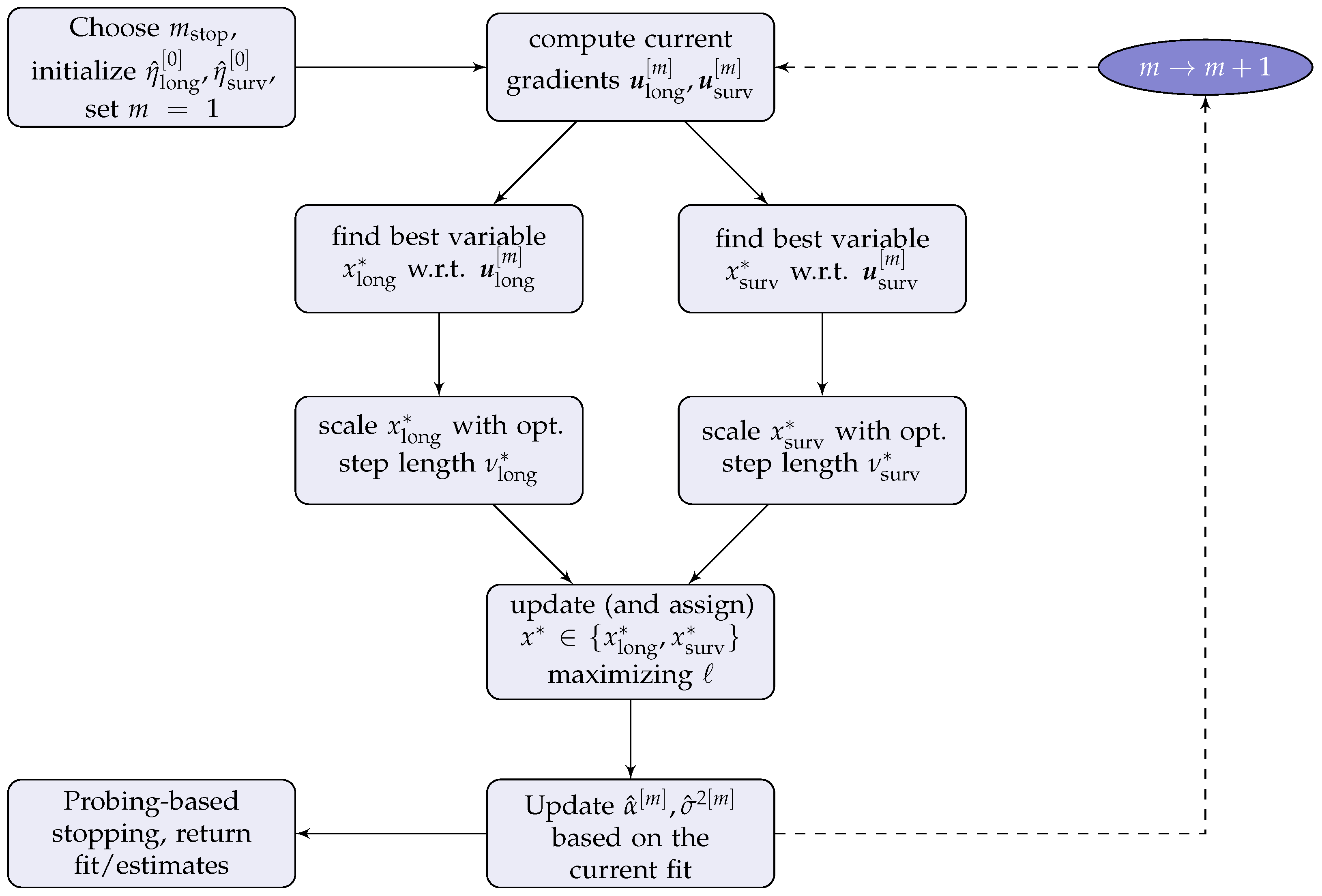
2.3. The JMalct Boosting Algorithm
| Algorithm 1: JMalct |
Compute the gradients Fit both gradients separately to the base-learners Compute the optimal step lengths , with corresponding likelihood values , and only update the component resulting in the best joint likelihood improvement: Update the active sets
Perform an additional longitudinal boosting update regarding the random structure: Obtain updates for the association by maximizing the joint likelihood:
|
2.4. Computational Details of the JMalct Algorithm
- while :
- G-step 1
- -
- Fit all base-learners to the longitudinal gradient with regard to ;
- -
- Find the best-performer, and corresponding step-length .
- G-step 2
- -
- Fit all base-learners to gradient with regard to ;
- -
- Find the best-performer, and corresponding step-length .
- L-step
- -
- Fit likelihood for and with updates from G1 and G2;
- -
- Select the best-performer and update corresponding sub-predictor;
- -
- Remove the selected candidate variable from options to choose for the other predictor (if not performed already).
- Step 4
- -
- Update based on the current fit.
3. Simulation Study
3.1. Setup
3.2. Selection and Allocation
3.3. Estimation Accuracy
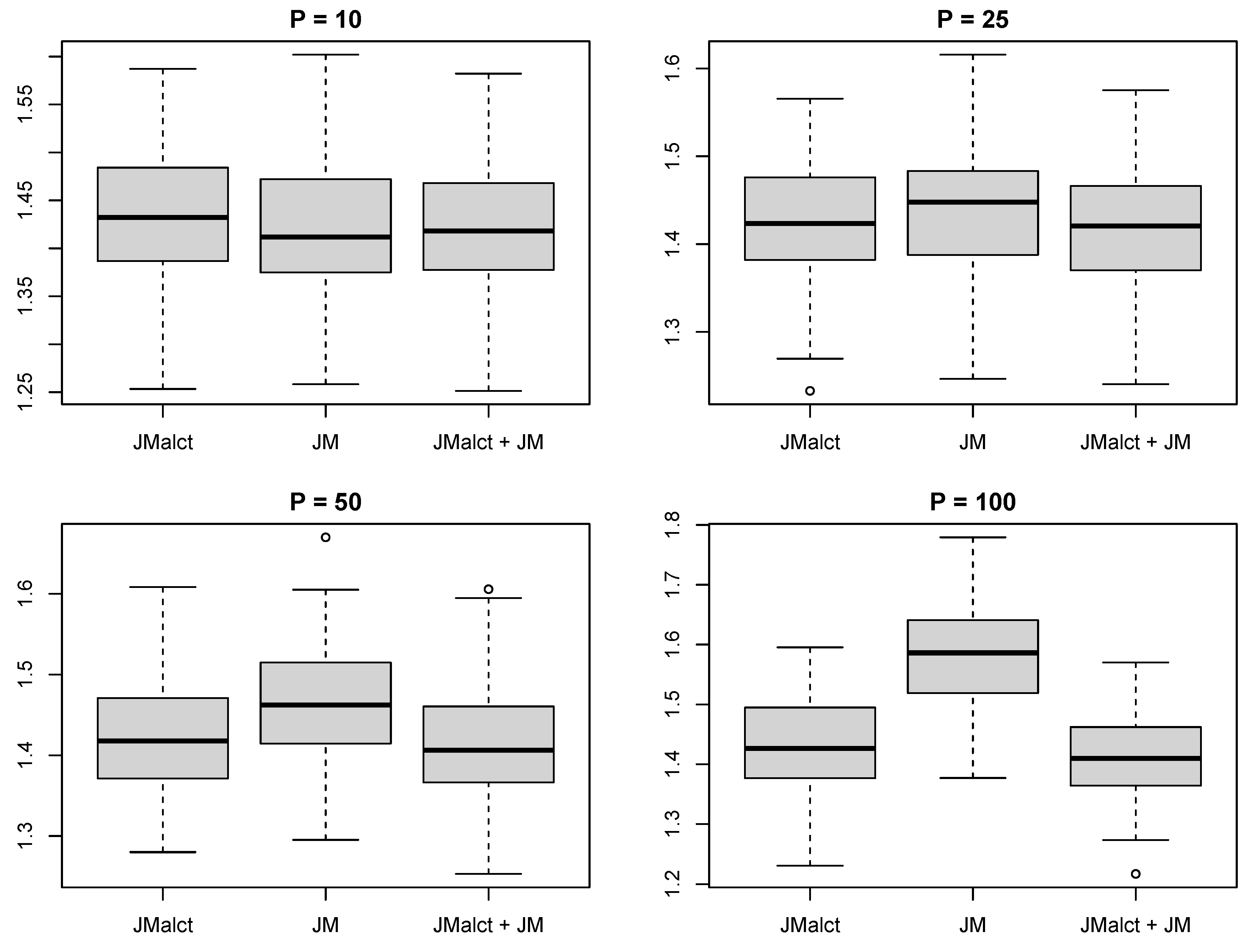
3.4. Predictive Performance
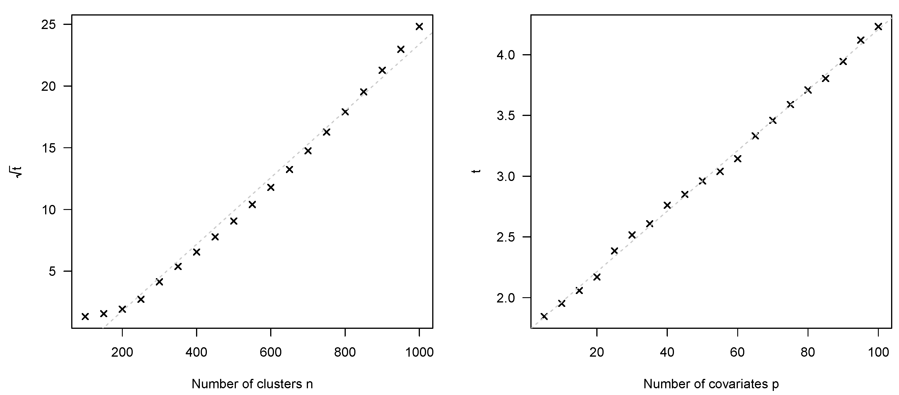
3.5. Computational Effort
3.6. Complexity
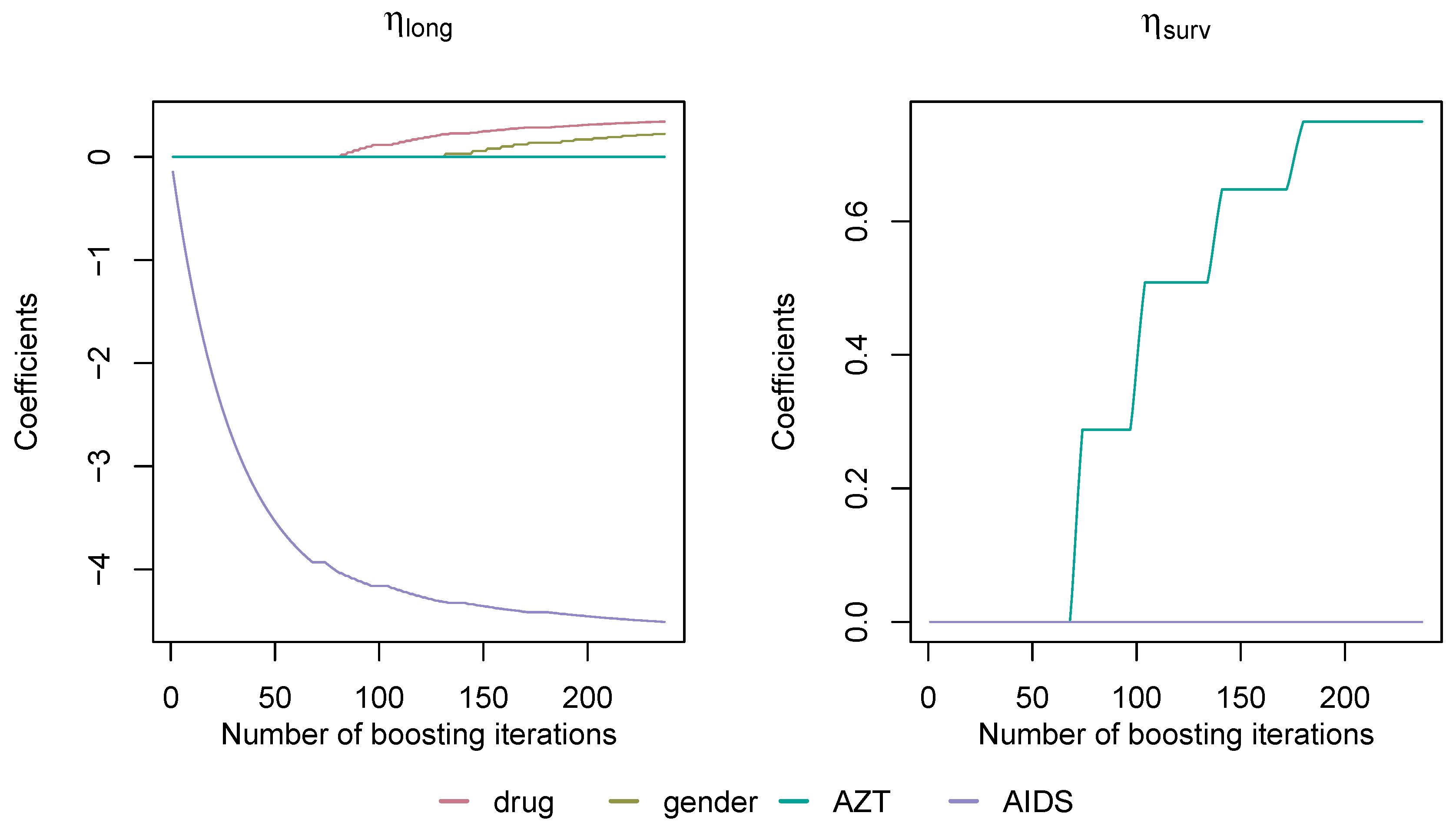
4. 1994 AIDS Study
5. Discussion and Outlook
Author Contributions
Funding
Data Availability Statement
Acknowledgments
Conflicts of Interest
Appendix A. Correction Matrix C
Appendix B. Simulation Algorithm
| Algorithm A1: simJM |
with and . Define hazard functions as described in Section 2.1.
according to inversion sampling.
|
References
- Wulfsohn, M.S.; Tsiatis, A.A. A Joint Model for Survival and Longitudinal Data Measured with Error. Biometrics 1997, 53, 330. [Google Scholar] [CrossRef] [PubMed]
- Rizopoulos, D. Joint Models for Longitudinal and Time-to-Event Data: With Applications in R; Chapman & Hall/CRC Biostatistics Series; CRC Press: Boca Raton, FL, USA, 2012; Volume 6. [Google Scholar]
- Rizopoulos, D. JM: An R Package for the Joint Modelling of Longitudinal and Time-to-Event Data. J. Stat. Softw. 2010, 35, 1–33. [Google Scholar] [CrossRef]
- Philipson, P.; Sousa, I.; Diggle, P.J.; Williamson, P.; Kolamunnage-Dona, R.; Henderson, R.; Hickey, G.L. JoineR: Joint Modelling of Repeated Measurements and Time-to-Event Data; R Package Version 1.2.6.; Springer: Berlin, Germany, 2018. [Google Scholar]
- Rizopoulos, D. The R Package JMbayes for Fitting Joint Models for Longitudinal and Time-to-Event Data Using MCMC. J. Stat. Softw. 2016, 72, 1–45. [Google Scholar] [CrossRef] [Green Version]
- Freund, Y.; Schapire, R.E. Experiments with a new boosting algorithm. In Proceedings of the Thirteenth International Conference on Machine Learning Theory, Bari, Italy, June 28–1 July 1996; Morgan Kaufmann: San Francisco, CA, USA, 1996; pp. 148–156. [Google Scholar]
- Freund, Y.; Schapire, R.E. A Decision-Theoretic Generalization of On-Line Learning and an Application to Boosting. J. Comput. Syst. Sci. 1997, 55, 119–139. [Google Scholar] [CrossRef] [Green Version]
- Friedman, J.; Hastie, T.; Tibshirani, R. Additive logistic regression: A statistical view of boosting (with discussion). Ann. Stat. 2000, 28, 337–407. [Google Scholar] [CrossRef]
- Bühlmann, P.; Hothorn, T. Boosting algorithms: Regularization, prediction and model fitting. Stat. Sci. 2007, 27, 477–505. [Google Scholar]
- Mayr, A.; Binder, H.; Gefeller, O.; Schmid, M. The Evolution of Boosting Algorithms - From Machine Learning to Statistical Modelling. Methods Inf. Med. 2014, 53, 419–427. [Google Scholar] [CrossRef] [Green Version]
- Mayr, A.; Fenske, N.; Hofner, B.; Kneib, T.; Schmid, M. Generalized additive models for location, scale and shape for high dimensional data-a flexible approach based on boosting. J. R. Stat. Soc. Ser. (Applied Stat.) 2012, 61, 403–427. [Google Scholar] [CrossRef] [Green Version]
- Waldmann, E.; Taylor-Robinson, D.; Klein, N.; Kneib, T.; Pressler, T.; Schmid, M.; Mayr, A. Boosting joint models for longitudinal and time-to-event data. Biom. J. 2017, 59, 1104–1121. [Google Scholar] [CrossRef] [Green Version]
- Griesbach, C.; Groll, A.; Bergherr, E. Joint Modelling Approaches to Survival Analysis via Likelihood-Based Boosting Techniques. Comput. Math. Methods Med. 2021, 2021, 4384035. [Google Scholar] [CrossRef]
- Tutz, G.; Binder, H. Generalized Additive Models with Implicit Variable Selection by Likelihood-Based Boosting. Biometrics 2006, 62, 961–971. [Google Scholar] [CrossRef] [PubMed]
- Rappl, A.; Mayr, A.; Waldmann, E. More than one way: Exploring the capabilities of different estimation approaches to joint models for longitudinal and time-to-event outcomes. Int. J. Biostat. 2021, 18, 127–149. [Google Scholar] [CrossRef] [PubMed]
- He, Z.; Tu, W.; Wang, S.; Fu, H.; Yu, Z. Simultaneous Variable Selection for Joint Models of Longitudinal and Survival Outcomes. Biometrics 2015, 71, 178–187. [Google Scholar] [CrossRef] [PubMed] [Green Version]
- Chen, Y.; Wang, Y. Variable selection for joint models of multivariate longitudinal measurements and event time data. Stat. Med. 2017, 36, 3820–3829. [Google Scholar] [CrossRef] [PubMed]
- Xie, Y.; He, Z.; Tu, W.; Yu, Z. Variable selection for joint models with time-varying coefficients. Stat. Methods Med. Res. 2019, 29, 309–322. [Google Scholar] [CrossRef]
- Tang, A.M.; Zhao, X.; Tang, N.S. Bayesian variable selection and estimation in semiparametric joint models of multivariate longitudinal and survival data. Biom. J. 2017, 59, 57–78. [Google Scholar] [CrossRef]
- Andrinopoulou, E.R.; Rizopoulos, D. Bayesian shrinkage approach for a joint model of longitudinal and survival outcomes assuming different association structures. Stat. Med. 2016, 35, 4813–4823. [Google Scholar] [CrossRef]
- Yi, F.; Tang, N.; Sun, J. Simultaneous variable selection and estimation for joint models of longitudinal and failure time data with interval censoring. Biometrics 2022, 78, 151–164. [Google Scholar] [CrossRef]
- Thomas, J.; Mayr, A.; Bischl, B.; Schmid, M.; Smith, A.; Hofner, B. Gradient boosting for distributional regression: Faster tuning and improved variable selection via noncyclical updates. Stat. Comput. 2017, 28, 673–687. [Google Scholar] [CrossRef] [Green Version]
- Zhang, B.; Hepp, T.; Greven, S.; Bergherr, E. Adaptive Step-Length Selection in Gradient Boosting for Generalized Additive Models for Location, Scale and Shape. Comput. Stat. 2022, 37, 2295–2332. [Google Scholar] [CrossRef]
- Griesbach, C.; Säfken, B.; Waldmann, E. Gradient boosting for linear mixed models. Int. J. Biostat. 2021, 17, 317–329. [Google Scholar] [CrossRef] [PubMed]
- Hepp, T.; Thomas, J.; Mayr, A.; Bischl, B. Probing for Sparse and Fast Variable Selection with Model-Based Boosting. Comput. Math. Methods Med. 2017, 2017, 1421409. [Google Scholar]
- Hofner, B. Variable Selection and Model Choice in Survival Models with Time-Varying Effects. Diploma Thesis, Ludwig-Maximilians-Universität München, Munich, Germany, 2008. [Google Scholar]
- Kneib, T.; Hothorn, T.; Tutz, G. Variable Selection and Model Choice in Geoadditive Regression Models. Biometrics 2009, 65, 626–634. [Google Scholar] [CrossRef] [PubMed] [Green Version]
- Griesbach, C.; Groll, A.; Bergherr, E. Addressing cluster-constant covariates in mixed effects models via likelihood-based boosting techniques. PLoS ONE 2021, 16, e0254178. [Google Scholar] [CrossRef]
- Bühlmann, P.; Yu, B. Boosting With the L2 Loss. J. Am. Stat. Assoc. 2003, 98, 324–339. [Google Scholar] [CrossRef]
- Bissantz, N.; Hohage, T.; Munk, A.; Ruymgaart, F. Convergence Rates of General Regularization Methods for Statistical Inverse Problems and Applications. SIAM J. Numer. Anal. 2007, 45, 2610–2636. [Google Scholar] [CrossRef] [Green Version]
- Yao, Y.; Rosasco, L.; Caponnetto, A. On Early Stopping in Gradient Descent Learning. Constr. Approx. 2007, 26, 289–315. [Google Scholar] [CrossRef]
- Bühlmann, P. Boosting for High-dimensional Linear Models. Ann. Stat. 2006, 34, 559–583. [Google Scholar] [CrossRef] [Green Version]
- Korn, E.; Simon, R. Measures of explained variation for survival data. Stat. Med. 1990, 9, 487–503. [Google Scholar] [CrossRef]
- Abrams, D.I.; Goldman, A.I.; Launer, C.; Korvick, J.A.; Neaton, J.D.; Crane, L.R.; Grodesky, M.; Wakefield, S.; Muth, K.; Kornegay, S.; et al. A Comparative Trial of Didanosine or Zalcitabine after Treatment with Zidovudine in Patients with Human Immunodeficiency Virus Infection. N. Engl. J. Med. 1994, 330, 657–662. [Google Scholar] [CrossRef]
- Meinshausen, N.; Bühlmann, P. Stability selection. J. R. Stat. Soc. Ser. (Stat. Methodol.) 2010, 72, 417–473. [Google Scholar] [CrossRef]
- Shah, R.D.; Samworth, R.J. Variable selection with error control: Another look at stability selection. J. R. Stat. Soc. Ser. (Stat. Methodol.) 2012, 75, 55–80. [Google Scholar] [CrossRef]
- Mayr, A.; Hofner, B.; Schmid, M. Boosting the discriminatory power of sparse survival models via optimization of the concordance index and stability selection. BMC Bioinform. 2016, 17, 288. [Google Scholar] [CrossRef] [PubMed] [Green Version]
- Zhang, T.; Yu, B. Boosting with early stopping: Convergence and consistency. Ann. Stat. 2005, 33, 1538–1579. [Google Scholar] [CrossRef]


| P | CAlong | IAlong | CAsurv | IAsurv | FP |
|---|---|---|---|---|---|
| 10 | 1.00 | 0.20 | 0.76 | 0.00 | 0.58 |
| 25 | 1.00 | 0.15 | 0.78 | 0.00 | 0.12 |
| 50 | 1.00 | 0.14 | 0.77 | 0.00 | 0.05 |
| 100 | 1.00 | 0.10 | 0.76 | 0.00 | 0.02 |
| P | JMalct | JM | JMalct+JM | ||||
|---|---|---|---|---|---|---|---|
| mselong | msesurv | mselong | msesurv | mselong | msesurv | ||
| 10 | 0.497 | 0.343 | 0.713 | 0.489 | 0.342 | 0.453 | |
| 25 | 0.479 | 0.296 | 1.888 | 1.359 | 0.309 | 0.417 | |
| 50 | 0.585 | 0.303 | 4.212 | 3.375 | 0.374 | 0.409 | |
| 100 | 0.563 | 0.295 | 9.532 | 9.483 | 0.320 | 0.393 | |
| 10 | 0.486 | 0.323 | 0.302 | 0.254 | 0.288 | 0.423 | |
| 25 | 0.470 | 0.292 | 0.247 | 0.291 | 0.239 | 0.398 | |
| 50 | 0.578 | 0.297 | 0.362 | 0.367 | 0.306 | 0.384 | |
| 100 | 0.557 | 0.290 | 0.315 | 0.558 | 0.254 | 0.373 | |
| P | JMalct | JM | JMalct+JM |
|---|---|---|---|
| 10 | 92.69 | 97.44 | 149.19 |
| 25 | 88.80 | 339.41 | 151.65 |
| 50 | 86.92 | 1009.52 | 152.59 |
| 100 | 85.06 | 3517.76 | 146.26 |
| y | T | t | Drug | Gender | AZT | prevOI | id | |
|---|---|---|---|---|---|---|---|---|
| 10.67 | 16.97 | 0 | 0 | ddC | male | intolerance | AIDS | 1 |
| 8.43 | 16.97 | 0 | 6 | ddC | male | intolerance | AIDS | 1 |
| 9.43 | 16.97 | 0 | 12 | ddC | male | intolerance | AIDS | 1 |
| 6.32 | 19.00 | 0 | 0 | ddI | male | intolerance | noAIDS | 2 |
| 8.12 | 19.00 | 0 | 6 | ddI | male | intolerance | noAIDS | 2 |
| 4.58 | 19.00 | 0 | 12 | ddI | male | intolerance | noAIDS | 2 |
| 5.00 | 19.00 | 0 | 18 | ddI | male | intolerance | noAIDS | 2 |
| 3.46 | 18.53 | 0 | 0 | ddI | female | intolerance | AIDS | 3 |
| 3.61 | 18.53 | 0 | 2 | ddI | female | intolerance | AIDS | 3 |
| 6.16 | 18.53 | 1 | 6 | ddI | female | intolerance | AIDS | 3 |
| ⋮ | ⋮ | ⋮ | ⋮ | ⋮ | ⋮ | ⋮ | ⋮ | ⋮ |
Disclaimer/Publisher’s Note: The statements, opinions and data contained in all publications are solely those of the individual author(s) and contributor(s) and not of MDPI and/or the editor(s). MDPI and/or the editor(s) disclaim responsibility for any injury to people or property resulting from any ideas, methods, instructions or products referred to in the content. |
© 2023 by the authors. Licensee MDPI, Basel, Switzerland. This article is an open access article distributed under the terms and conditions of the Creative Commons Attribution (CC BY) license (https://creativecommons.org/licenses/by/4.0/).
Share and Cite
Griesbach, C.; Mayr, A.; Bergherr, E. Variable Selection and Allocation in Joint Models via Gradient Boosting Techniques. Mathematics 2023, 11, 411. https://doi.org/10.3390/math11020411
Griesbach C, Mayr A, Bergherr E. Variable Selection and Allocation in Joint Models via Gradient Boosting Techniques. Mathematics. 2023; 11(2):411. https://doi.org/10.3390/math11020411
Chicago/Turabian StyleGriesbach, Colin, Andreas Mayr, and Elisabeth Bergherr. 2023. "Variable Selection and Allocation in Joint Models via Gradient Boosting Techniques" Mathematics 11, no. 2: 411. https://doi.org/10.3390/math11020411