Article

A Multi-Objective Optimization Method for Flexible Job Shop Scheduling Considering Cutting-Tool Degradation with Energy-Saving Measures

1
Key Laboratory of Mechanism Theory and Equipment Design of Ministry of Education, Tianjin University, Tianjin 300072, China
2
School of Mechanical Engineering, Tianjin University, Tianjin 300072, China
3
School of Mechanical Engineering, Tianjin University of Commerce, Tianjin 300134, China
4
Tianjin Tianshen Intelligent Equipment Co., Ltd., Tianjin 300300, China
*
Authors to whom correspondence should be addressed.
Mathematics 2023, 11(2), 324; https://doi.org/10.3390/math11020324
Submission received: 12 December 2022 / Revised: 4 January 2023 / Accepted: 6 January 2023 / Published: 8 January 2023

Abstract

:
Traditional energy-saving optimization of shop scheduling often separates the coupling relationship between a single machine and the shop system, which not only limits the potential of energy-saving but also leads to a large deviation between the optimized result and the actual application. In practice, cutting-tool degradation during operation is inevitable, which will not only lead to the increase in actual machining power but also the resulting tool change operation will disrupt the rhythm of production scheduling. Therefore, to make the energy consumption calculation in scheduling optimization more consistent with the actual machining conditions and reduce the impact of tool degradation on the manufacturing shop, this paper constructs an integrated optimization model including a flexible job shop scheduling problem (FJSP), machining power prediction, tool life prediction and energy-saving strategy. First, an exponential function is formulated using actual cutting experiment data under certain machining conditions to express cutting-tool degradation. Utilizing this function, a reasonable cutting-tool change schedule is obtained. A hybrid energy-saving strategy that combines a cutting-tool change with machine tool turn-on/off schedules to reduce the difference between the simulated and actual machining power while optimizing the energy savings is then proposed. Second, a multi-objective optimization model was established to reduce the makespan, total machine tool load, number of times machine tools are turned on/off and cutting tools are changed, and the total energy consumption of the workshop and the fast and elitist multi-objective genetic algorithm (NSGA-II) is used to solve the model. Finally, combined with the workshop production cost evaluation indicator, a practical FJSP example is presented to demonstrate the proposed optimization model. The prediction accuracy of the machining power is more than 93%. The hybrid energy-saving strategy can further reduce the energy consumption of the workshop by 4.44% and the production cost by 2.44% on the basis of saving 93.5% of non-processing energy consumption by the machine on/off energy-saving strategy.

1. Introduction

In the current industrial environment, the manufacturing industry, as an important part, consumes a lot of energy and resources in the process of product manufacturing [1]. The report on power consumption released by the China Electricity Council in 2022 showed that China’s industrial electricity consumption accounted for 64.5% of the total social electricity consumption in the first 10 months of 2022, while manufacturing electricity consumption accounted for 76% of industrial electricity consumption. In addition, research shows that 99% of environment-related problems in mechanical processes are due to electrical energy consumption [2]. Therefore, the establishment of an energy-saving machining system is an urgent requirement to reduce environmental impacts and every manufacturing enterprise needs to focus on it.
Energy-saving strategies using new materials and technologies may require enterprises to transform and invest a lot in existing manufacturing systems, therefore enterprises are usually inclined to carry out energy-saving scheduling and management [3]. Through scientific matching of production tasks and machine tools, more accurate calculation of tasks sequencing, reduce idle time of machine tools, and reasonable selection of machine tools on/off time can improve energy efficiency [4]. Additionally, Guzman et al. indicated that a gap still exists in developing mathematical models to deal with scheduling problems. Novel modeling approaches should be developed to address and associate the parameters related to production and sustainability [5], among which Feng et al. integrated multiple optimization algorithms and apply edge artificial intelligence (AI) to smart green scheduling of sustainable flexible shop floors [6]. Guzman et al. provided a mixed integer linear programming (MILP) model to address the multi-machine CLSD-BPIM (a capacitated lot-sizing problem with sequence-dependent setups and parallel machines in a bi-part injection molding) [7]. Mula et al. proposed a matheuristic algorithm to optimize the job-shop problem, which combines a genetic algorithm with a disjunctive mathematical model to cut computational times, and the Coin-OR Branch and Cut open-source solver is employed [8]. Rakovitis et al. developed a novel mathematical formulation for the energy-efficient flexible job-shop scheduling problem using the improved unit-specific event-based time representation and proposed a grouping-based decomposition approach to efficiently solve large-scale problems [
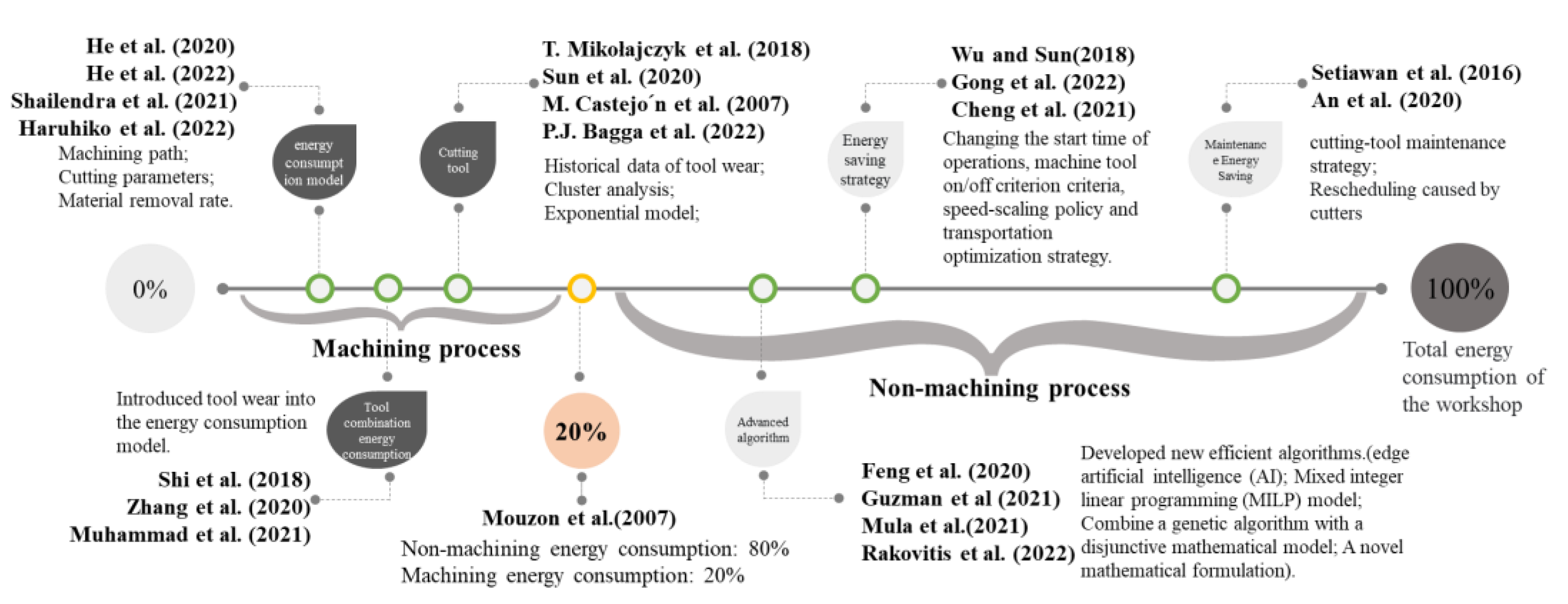
9]. Knowing that approximately 80% of the energy consumption of machine tools is attributed to non-processing operations, whereas the actual energy consumed by processing operations accounts for less than 20% [10]. If only relying on advanced algorithms to achieve further energy saving in the workshop, the effect is limited. Wu and Sun realized energy saving by changing the turning on/off time of machine tools and choosing different machining speeds [11]. Gong et al. effectively reduced the number of machine restarts and total energy consumption by changing the start time of operations on different machines [12]. Cheng et al. proposed machine tool on/off criterion criteria, speed-scaling policy and transportation optimization strategy, and applied them to manufacturing unit scheduling problems to achieve overall energy saving [13]. An et al. proposed a worn cutting-tool maintenance strategy that reduced the impact of cutting-tool degradation and the total energy consumption of cutting-tool maintenance in manufacturing workshops [14]. Setiawan et al. studied a shop rescheduling problem caused by the failure or reduced service life of cutting tools [15].
As can be seen from the aforementioned literature, on the one hand, most energy-saving scheduling problems start from the perspective of improving the performance of the algorithm, which makes the optimization calculation of shop energy consumption more accurate. However, on the other hand, from the perspective of workshop system management to achieve energy saving, in order to further realize the energy saving of the manufacturing system, it is important to consider the contribution of the coupling relationship between the energy consumption of individual equipment and the energy consumption of the system to the actual production and optimization objectives; however, this was almost ignored in previous studies. As the basic energy consumption equipment in the manufacturing process [16], the energy consumption caused by machine tools cannot be ignored. However, accurate estimation of energy consumption is the basis for improving energy efficiency. In recent years, different modeling methods for machine tool energy consumption have been proposed, such as those by He et al. and He et al., who combined the tool machining path with the energy consumption model to improve machining efficiency [17,18]. Shailendra et al. established an empirical model between cutting parameters and energy consumption of end turning by experiments [19]. Haruhiko et al. proposed an empirical model for predicting machine tool power consumption based on the power function between specific energy consumption and material removal rate [20]. In addition, as the direct implementer of machine tool cutting, tool changing and maintenance will directly affect the production schedule, in order to avoid the tool suddenly reaching the end of life, resulting in the conflict of resources, energy consumption increase and the extension of the makespan and other problems. T. Mikołajczyk et al. and Sun et al. established the prediction model of tool residual life based on the historical data of tool wear [21,22]. M. Castejo’n et al. and P.J. Bagga et al. constructed a tool wear image dataset to predict tool life using cluster analysis and an exponential model [23,24]. Shi et al., Zhang et al. and Muhammad et al. introduced tool wear into the energy consumption model to achieve accurate energy consumption modeling, which laid a foundation for the integration of tool life prediction and energy consumption model [25,26,27]. Figure 1 summarizes the above literature.
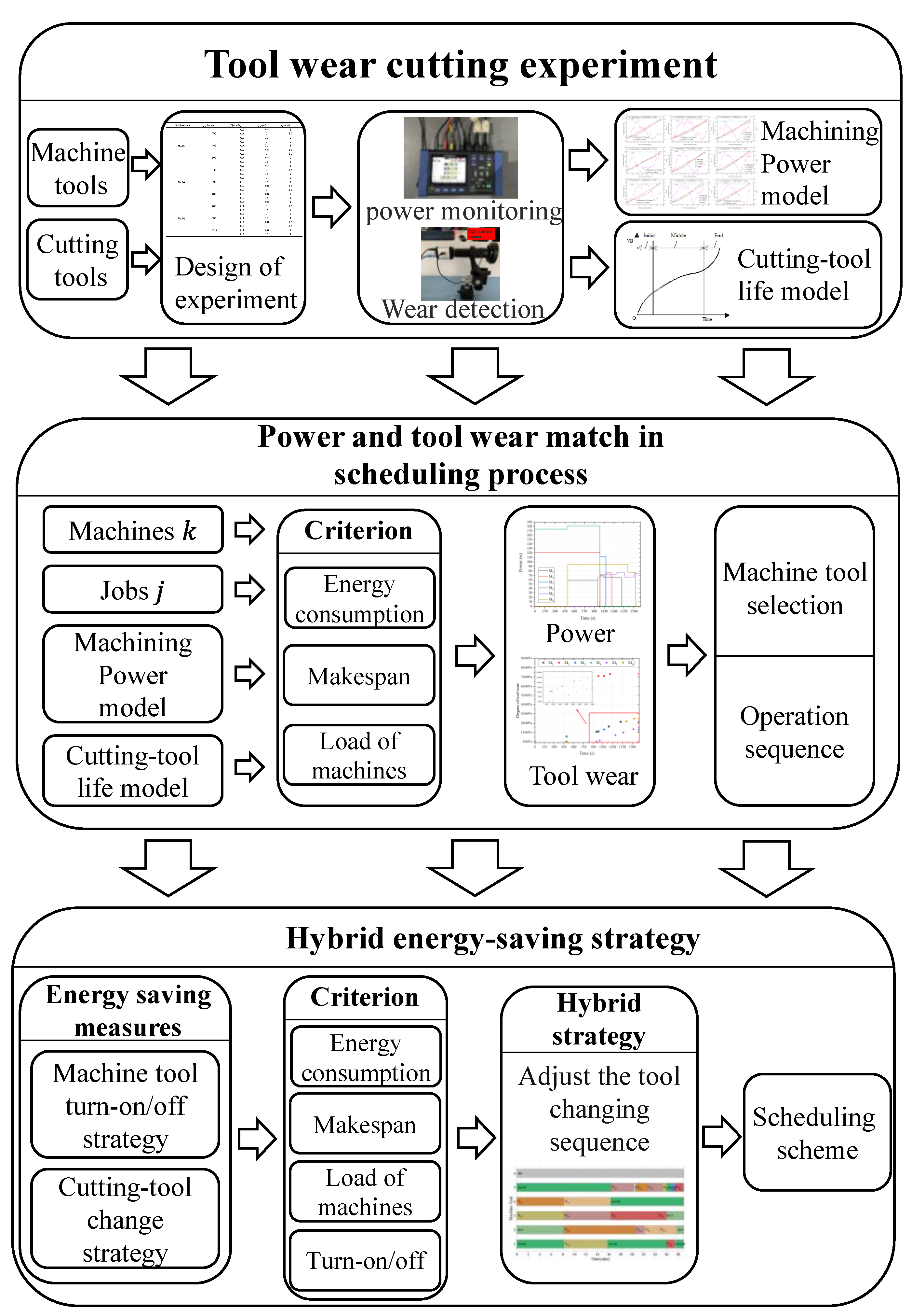
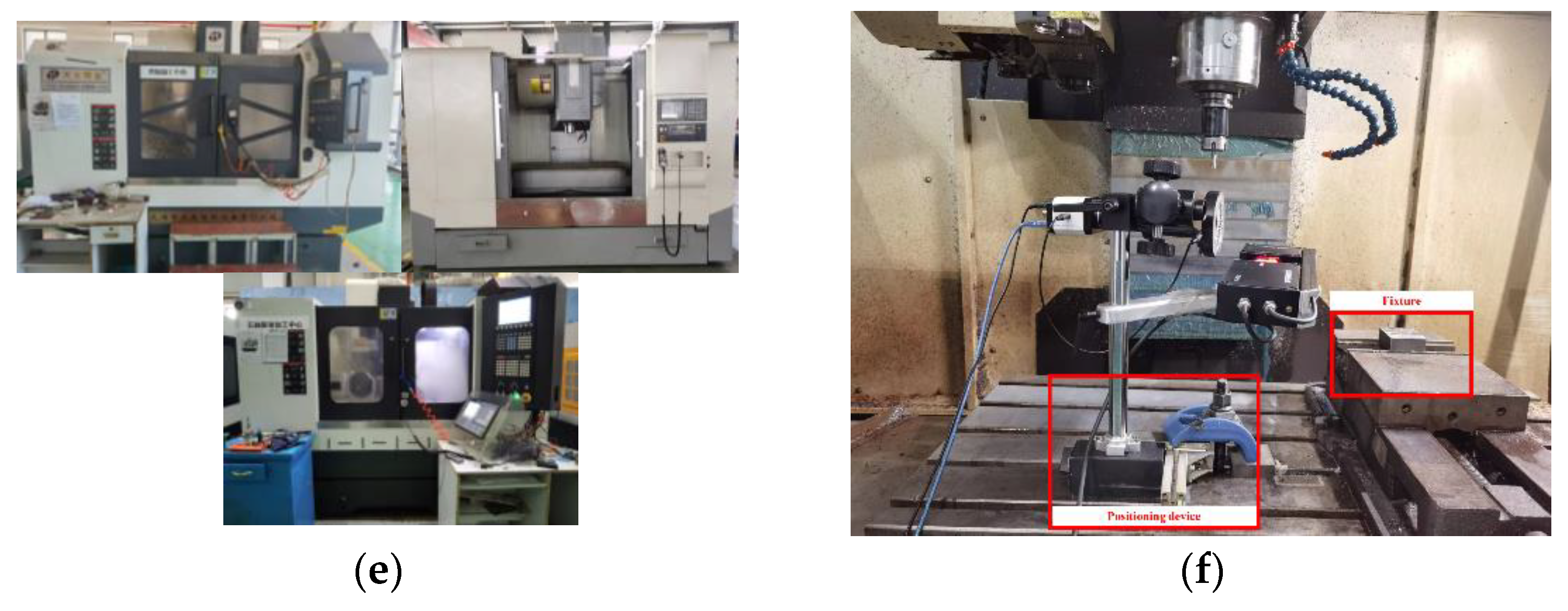
In summary, few researchers combine shop scheduling under low-carbon production with single-machine tool energy consumption and tool life prediction. This paper analyzes the coupling relationship between shop scheduling, single-machine tool energy consumption and tool life prediction, and organically integrates the three to achieve deeper shop consumption reduction. Firstly, the machining power model and the tool life model of the machine tool were established through the tool wear-cutting experiment. Then, the two models were integrated into the shop scheduling system to obtain the machining power of each production procedure and the tool change time of each machine tool in the shop scheduling process, so as to realize the precise modeling of energy consumption at the system level. In addition, on the basis of the machine tool turn-on/off strategy of the workshop, considering the relationship between the tool change time and the turn-on/off time of the machine tool, the tool change time is adjusted to further reduce the machining power and the makespan of the workshop, so as to reduce the production energy consumption of the workshop, as shown in Figure 2.
The remainder of the paper is organized as follows. Section 2 describes the FJSP, cutting-tool degradation model, and hybrid energy-saving strategy of cutting-tool change and machine tool turn-on/off. In Section 3, a multi-objective optimization model of flexible job shop scheduling is established that considers tool degradation and energy-saving measures. 
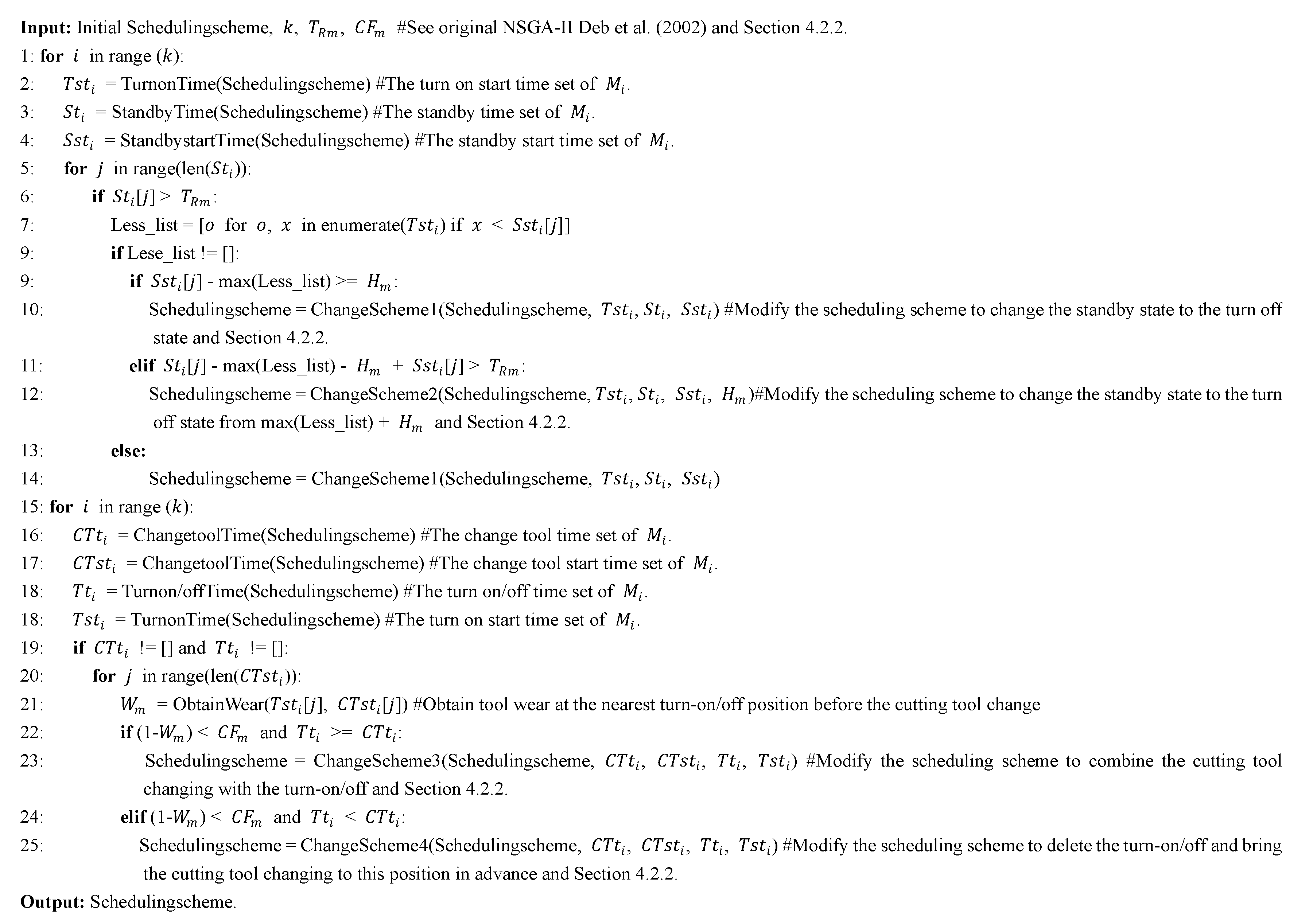
Section 4 introduces the proposed NSGA-II algorithm and its specific improvements. Section 5 sets the optimization model parameters through data collection and the analysis of actual cases. The rationality, effectiveness, and practical effects of the proposed model and algorithm are analyzed through verification experiments. Section 6 presents the conclusions and directions for future study.

2. Problem Description

The relevant symbols are provided in this section. Then, the FJSP that considers cutting-tool degradation with energy-saving measures (FJSP–CTD–ESM) is described. First, the FJSP is described. Then, the calculation method of the cutting-tool life, dynamic machining power, and the hybrid energy-saving strategy of cutting-tool change and machine tool turn-on/off is proposed, which combines the cutting-tool degradation and machine tool turn-on/off effects.

2.1. FJSP Description
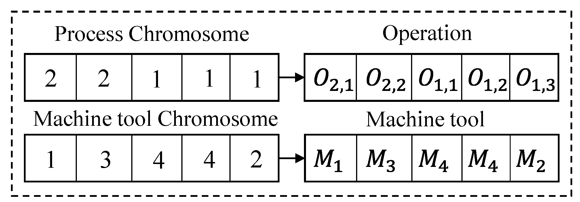
In the FJSP, there are n kinds of jobs J = { J i } i = 1 , 2 , , n and k machine tools M = { M m } m = 1 , 2 , , k , and each job J i   has S i preset sequence of operations O = { o i , j } j = 1 , 2 , , S i (Li et al., 2012). At least one operation o i , j in O can be processed by different machine tools, with a corresponding difference in the processing time and efficiency for the same operation.
The following conditions should be met in the FJSP: (1) A machine tool cannot be assigned to two or more operations simultaneously. (2) Each job has the same processing priority: initially, all jobs can be processed. (3) There is no constraint relationship between different jobs. (4) The optional machine tools for the job have no priority relationship. (5) All job processing tasks are non-preemptive. (6) The processing power of the machine tool and degree of cutting-tool wear obey the law of tool degradation. (7) Once a process begins, it cannot be interrupted before completion. Changing the cutting tool and turning the machine tool on/off cannot be inserted into the machining process. (8) The conversion time between different jobs with the same machine tool as well as the transportation time between different stages of the same job are ignored.
The symbols used in this paper are defined in Table 1.

2.2. Cutting-Tool Degradation Model

In the FJSP, the degradation of the cutting tool reduces its machining capacity, leading to an increase in the machining power and the interruption of the process caused by the blunt cutting tool. If the cutting-tool wear is considered in advance during the scheduling process, the change in machining power caused by cutting-tool wear can be accurately predicted. This not only improves processing efficiency and reduces energy consumption but also prevents the cutting tool from becoming blunt.
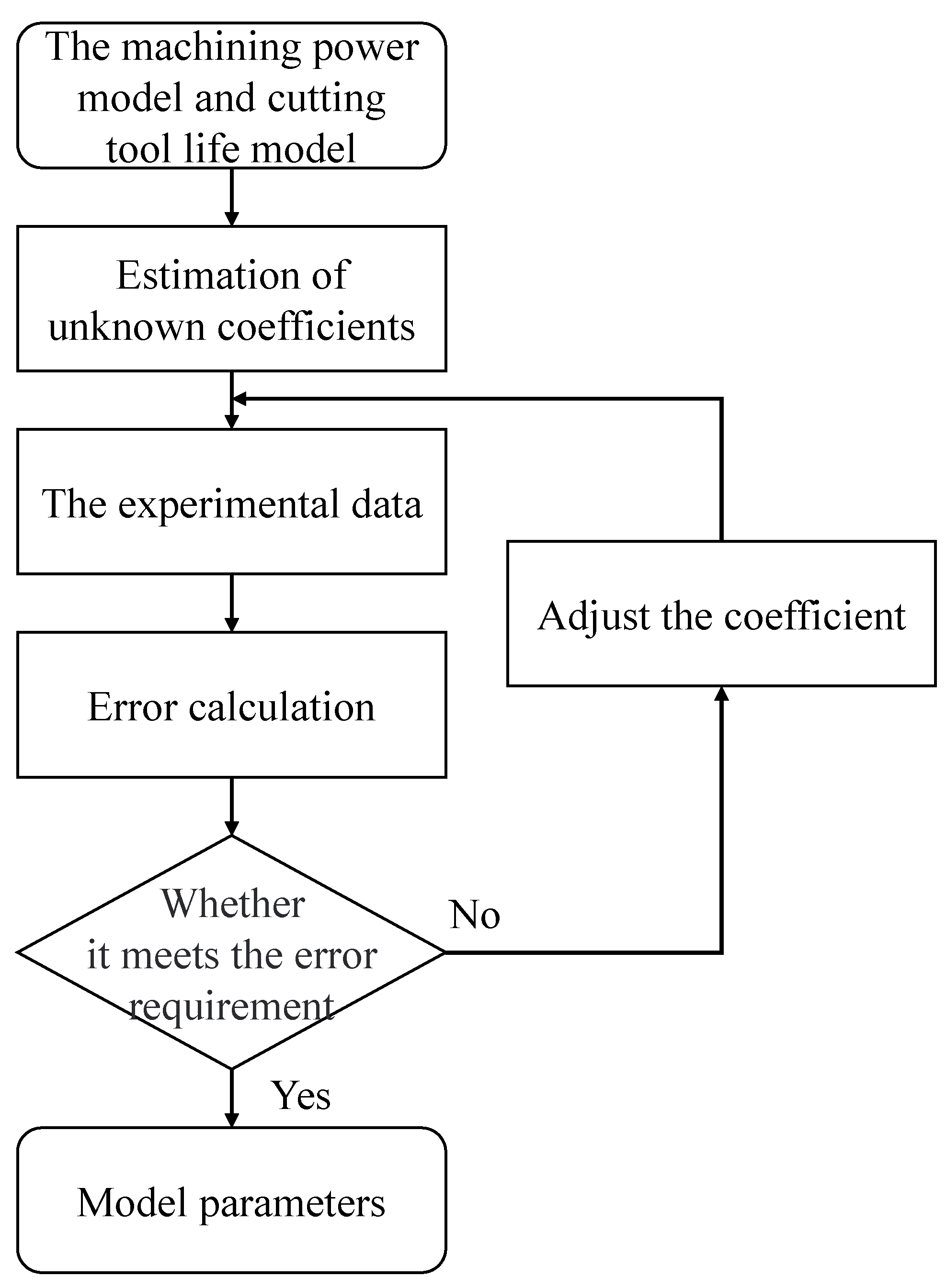
This section introduces the machining power model and cutting-tool life model derived from the tool degradation model.
(1) Machining power model
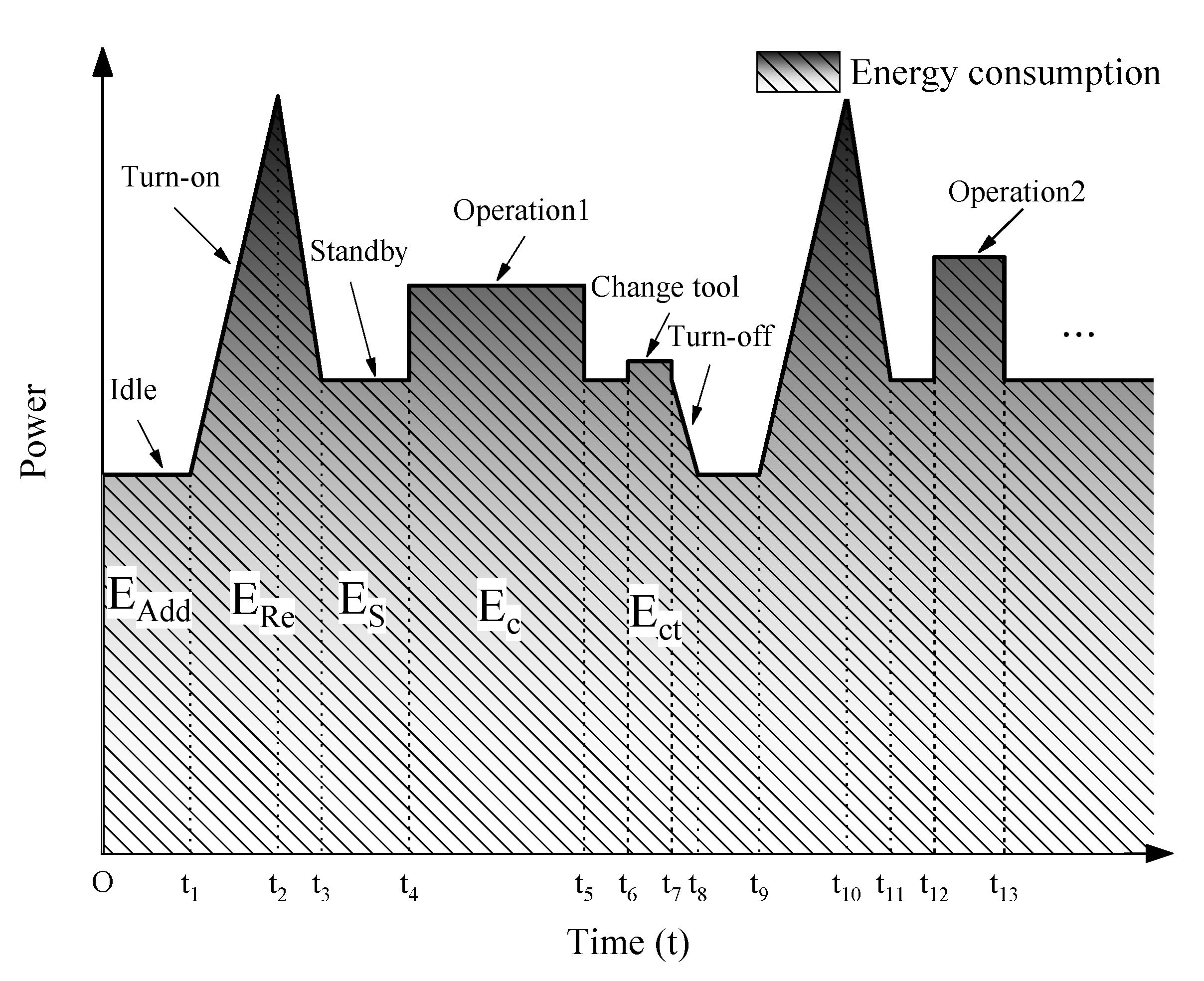
From the point of view of the working state of the machine tool, the machine tool power P m in the workshop production process can be divided into two parts, as shown in Equation (1). The first part is the dynamic machining power of the machine tool P d m , which includes the spindle power of the machine tool in the workpiece-cutting process. The second part is the static power P s m of the machine tool, including the no-load power of the motor and the power of the numerical control, lighting, and cooling systems.
P m = P d m + P s m ,
P s m exhibits little change in the machining process; hence, it is regarded as a constant value.
The dynamic power model [28,29] proposed by Tian et al. and Tian et al. is divided into two parts: the initial dynamic power without tool wear, and the additional dynamic power caused by tool wear, as shown in Equation (2):
P d m = K 1 n v a 1 f a 2 a p a 3 a e a 4 + K 2 t m n a 5 f a 6 a p a 7 a e a 8
(2) Cutting-tool life model
To determine the relationship between the cutting-tool life and different cutting parameters, a type of cutting-tool failure should be selected as the criterion. According to ISO 8688-2:1989 Tool life testing in milling-part 2: end milling (1989), the wear of an end milling cutter can be divided into rake-face wear and flank-face wear [30]. Because the flank-face wear is easy to measure, the blunt standard of the tool wear is often set according to the maximum allowable value of the flank-face wear (usually expressed as VB). In this study, the end of the end milling cutting tool’s life was defined as having a maximum VB of 0.3 mm in one of all teeth (VBmax = 0.3). The cutting-tool life model of Tian et al. and Sun et al. is shown in Equation (3) [22,29]:
T m = K 3 · n v b 1 f b 2 a e b 3 a e b 4
As we all know, tool wear is produced in complex mechanical and thermal environments, and there will be different dullness criteria for different processing objects or different quality requirements. In this paper, according to the dullness criterion mentioned in the ISO standard, in other application scenarios with higher cutting quality requirements, this part of modeling needs to establish a dullness criterion that meets the quality requirements and build models under these standards. This article only provides such a solution.

2.3. The Hybrid Energy-Saving Strategy

Section 2.2 shows that the cutting-tool life is not only related to the material and specifications of the cutting tool but also to the cutting parameters. Therefore, the cutting tool remaining useful life (RUL) cannot be calculated directly from the processing time of different operations. This results in a unique tool-changing schedule that affects the makespan and machine tool turn-on/off schedule.
Three measures are proposed to solve this problem.
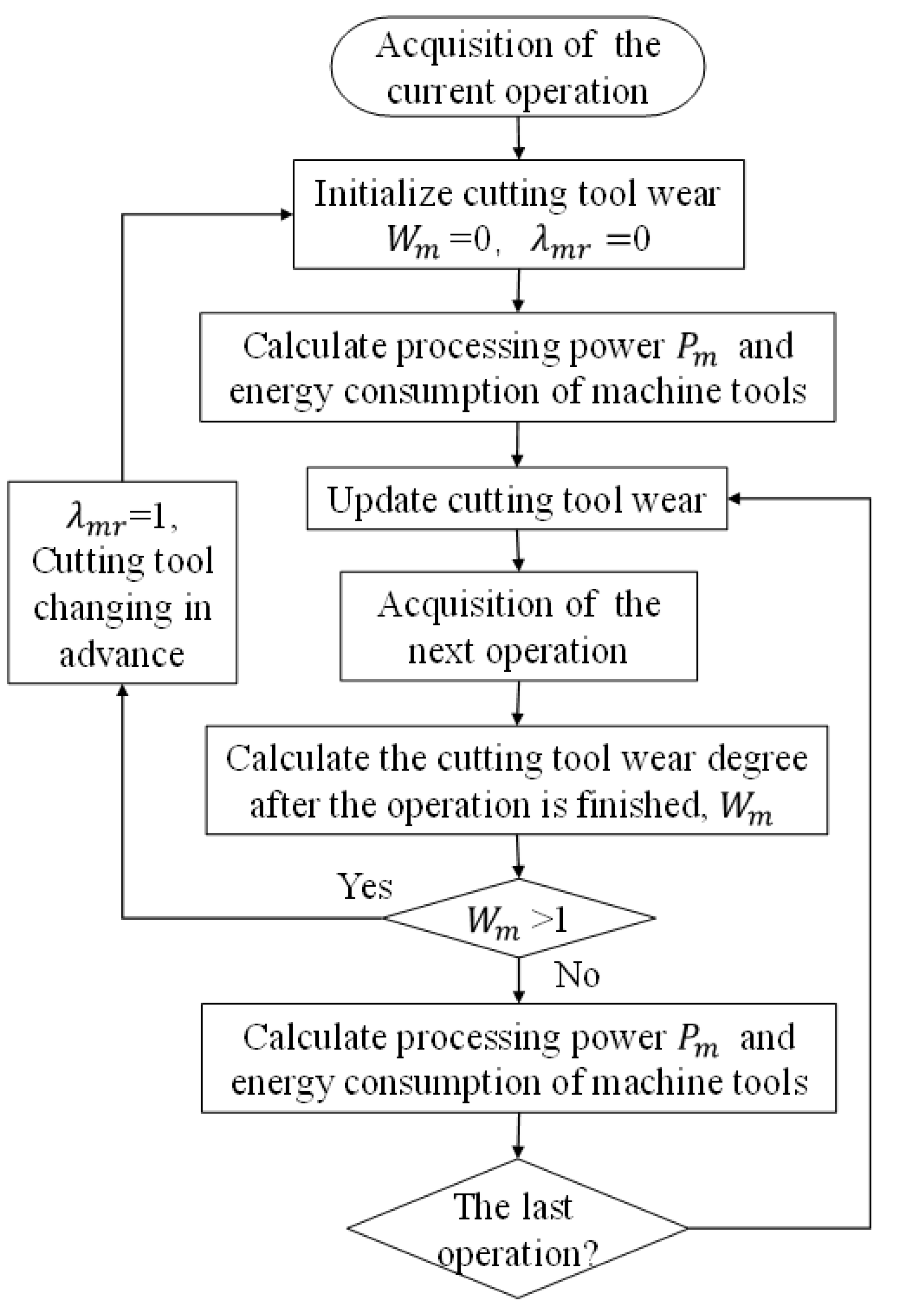
(1) The cutting-tool change strategy
In this study, the cutting tool is changed before it is damaged to ensure that it meets processing quality requirements, reduces the risk of accidents, and improves the reliability of the processing system. Therefore, if the remaining service life of the cutting tool is insufficient to support the next processing task in the schedule, the cutting tool is considered unavailable and changed before the start of the next processing task, as expressed by Equation (4).
T m t m < P T
Owing to the different cutting-tool lives under different cutting parameters, the cutting-tool service time cannot be added directly. A normalized approach is adopted to deal with this problem, that is, the increase in cutting-tool wear caused by the processing task is obtained using the processing task time / cutting-tool life under the cutting parameters of the task. Then, the total cutting-tool wear W m is used to determine whether the cutting tool has reached the end point of its service life, as expressed by Equation (5).
W m + P T /   T m < 1
Equation (5) defines that cutting-tool wear must be less than 1.
(2) The machine tool turn-on/off strategy
During the production process, if a machine tool remains idle for some time, it is sensible to turn it off to avoid wasting energy and reduce carbon emissions. Turning machine tools on/off leads to additional energy consumption and could also damage their performance and service life. Therefore, the no-load balance time   T R m should be set to control when to turn the machine tool on/off, as expressed by Equation (6). Meanwhile, to reduce the damage caused by turning the machine tool on/off, the interval between on/off times is controlled by setting the on/off security threshold time H m , as expressed by Equation (7) [11].
S T m r C T m ( r 1 ) T R m η m r
| η m r C T m ( r 1 ) η m r S T m r | H m δ m ,     r > r
Equation (6) shows that if the time interval between two subsequent processing tasks is greater than the no-load balancing time, the machine tool should be turned off. Equation (7) shows that if the machine tool is turned on/off twice or more, the interval between the time the machine tool is turned on and the next turn-off must exceed the on/off security threshold time of the machine tool.
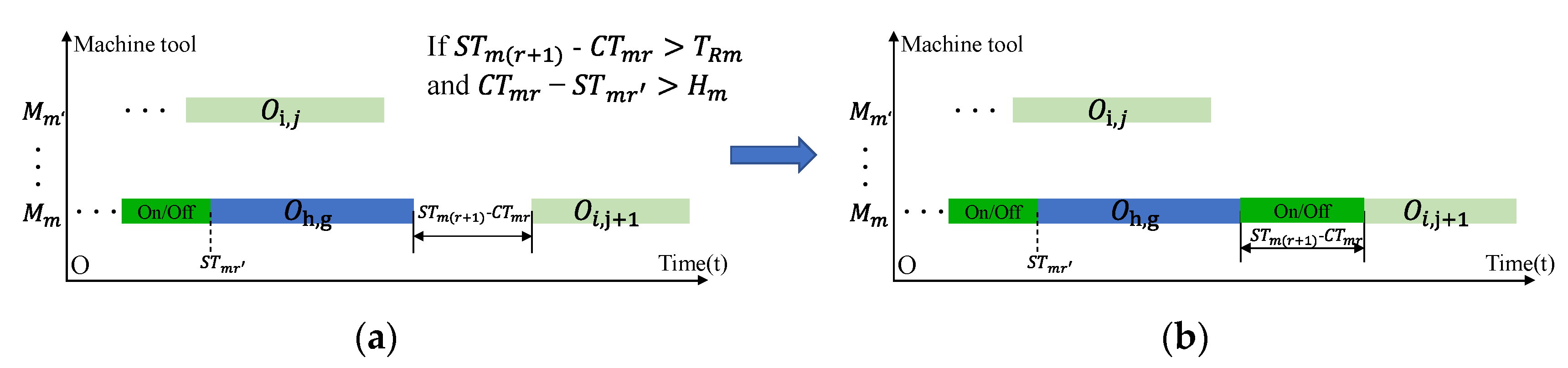
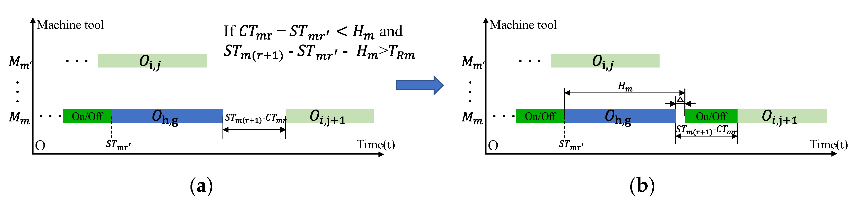
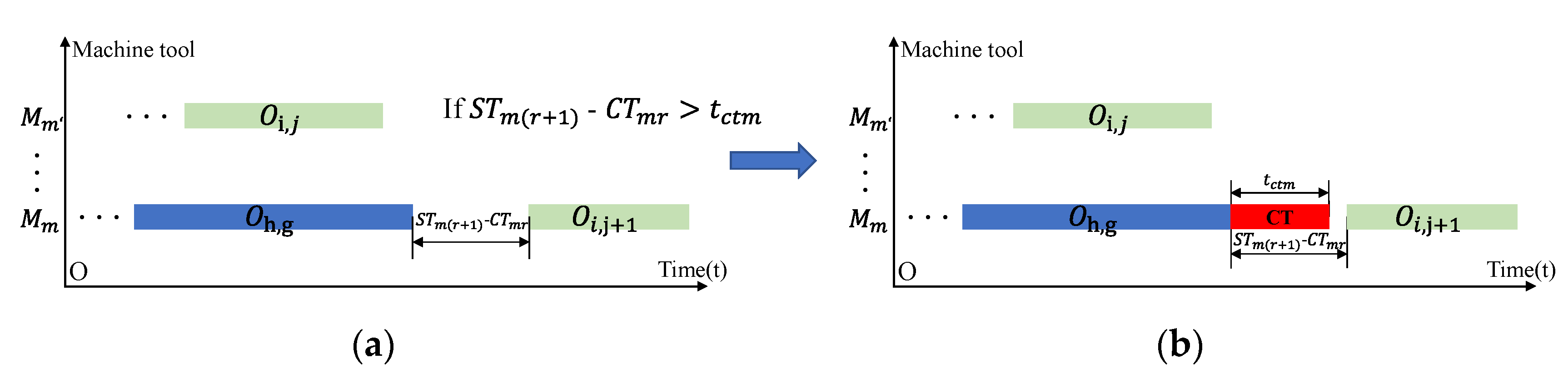
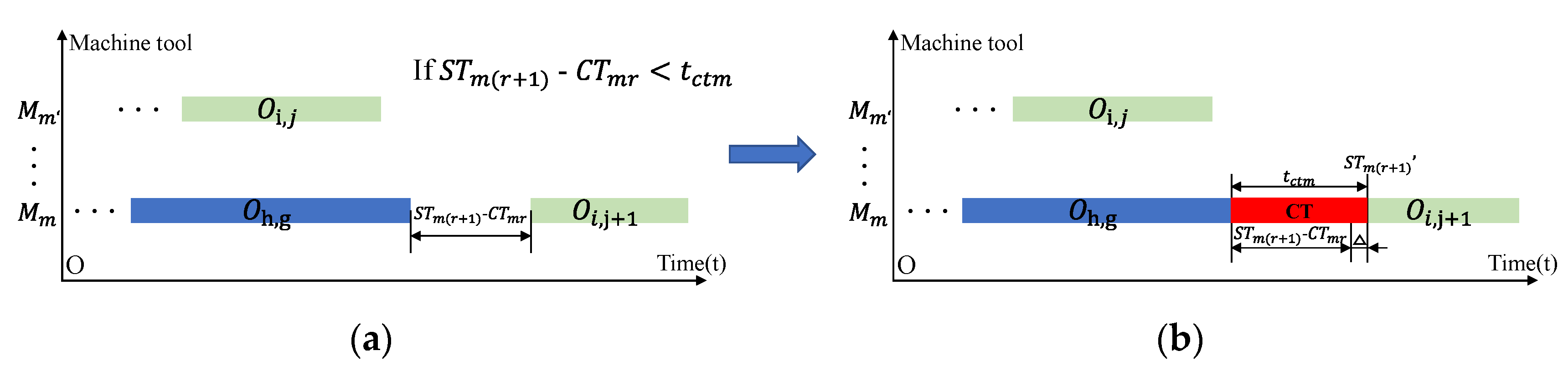
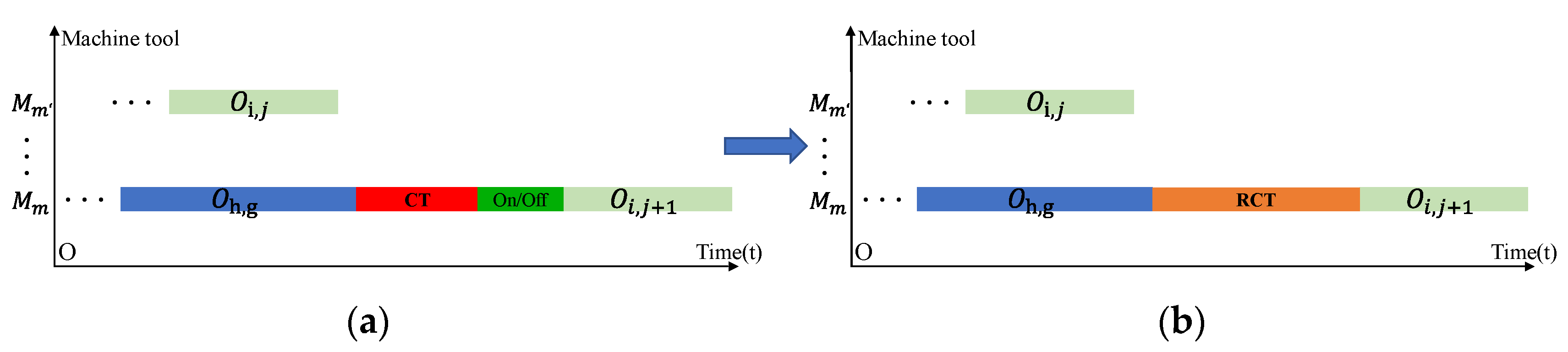
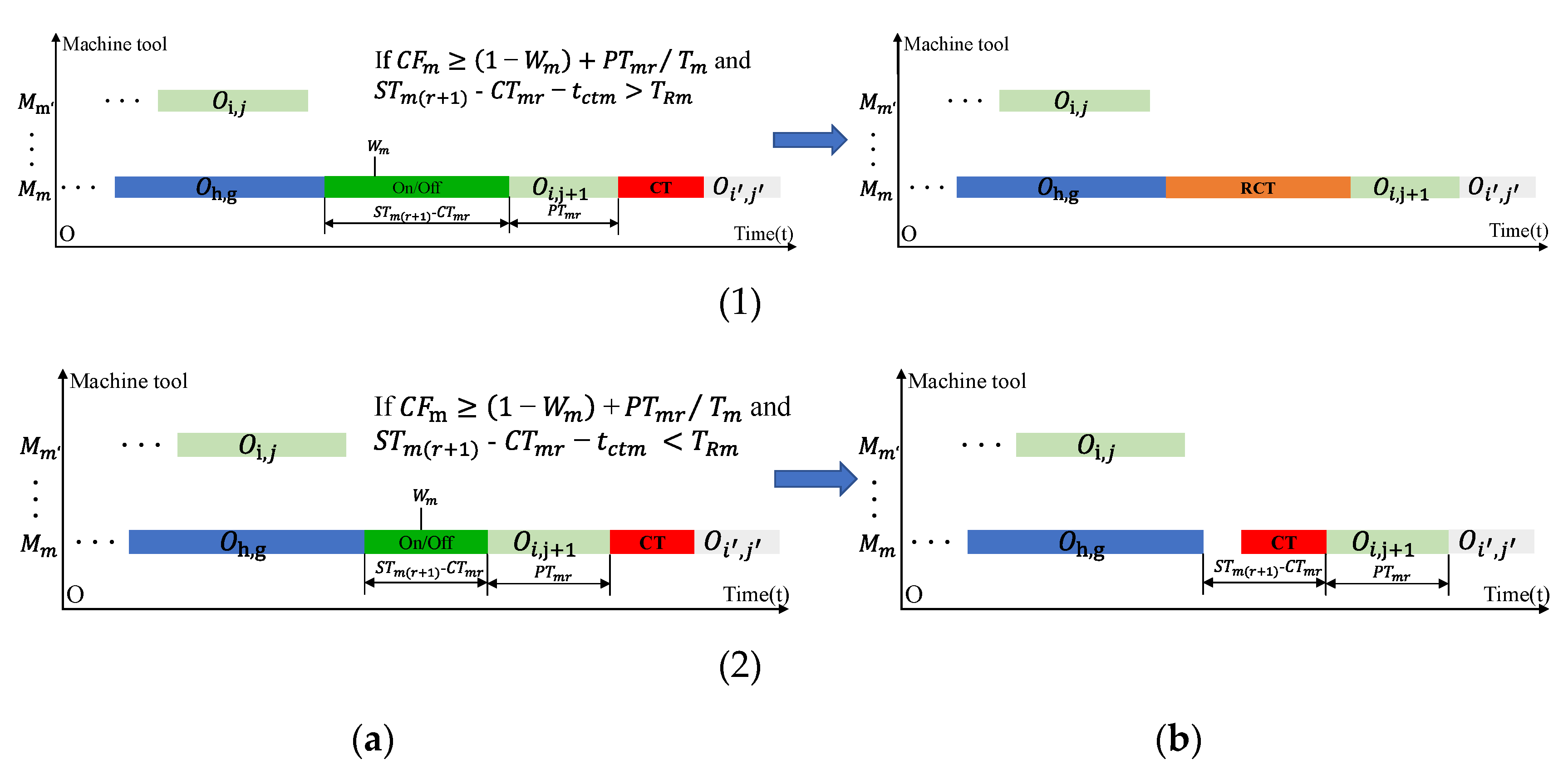
(3) Hybrid energy-saving strategy of cutting-tool change and machine tool turn-on/off
If the cutting-tool change operation is separated from the machine tool turn-on/off operation, the single cutting-tool change operation not only increases the makespan but also the standby energy consumption of the machine tool. Sacrificing a small amount of cutting-tool processing capacity by advancing the timing of the cutting-tool change will shorten the makespan and reduce energy consumption. Here, we set a reasonable coefficient C F m of the cutting-tool capacity to control when to change the cutting tool. Equation (8) ensures that the reduced processing capacity of the machine tool M m is within an acceptable range. The cutting-tool change operation can be carried out before x tasks to realize energy savings.
C F m 1 W m + r = 0 x ( λ m r P T m r /   T m )

3. Formulation of FJSP–CTD–ESM

In this section, the energy footprint model is defined. Then, the optimization model of the FJSP–CTD–ESM is established.

3.1. Energy Footprint Model

The total energy consumption E t o t a l of the workshop consists of five parts, as shown in Equation (9). Figure 3 shows the energy consumption of the machine tool at different stages [1].
E total = E C + E Re + E ct + E S + E Add
The energy consumption of each part is analyzed in detail below.
(1) Processing energy consumption E c of machine tools
The processing energy consumption E c of process o i , j is closely related to the cutting time P T i j m and the machine tool power P i j m , which varies with the machine tool type, cutting parameters, and cutting-tool wear. The energy consumption of cutting is calculated as Equation (10).
E c = m = 1 k i = 1 n j = 1 S i r = 1 l m γ i j m r P i j m P T i j m
(2) Energy consumption E R e of turning machine tools on/off
The energy consumption when turning the machine tool on/off E R e is influenced by the type and performance of the machine tool; it has no relation with the processing operation. Thus, the energy consumption of turning the machine tool on/off E R e m once was set as a constant value. The energy consumption of machine tool turn-on/off is calculated as Equation (11).
E R e = m = 1 k r = 1 l m η m r E R e m
(3) Total energy consumption E c t of changing the cutting tool
As the processing time increases, it is necessary to change the cutting tool before it becomes blunt. The energy consumption of cutting-tool change is calculated as Equation (12).
E c t = m = 1 k r = 1 l m λ m r P c t m t c t m
(4) Standby energy consumption E s
When the machine tool is idle and kept on between two processes, it consumes energy while on standby, which is expressed as:
E s = m = 1 k r = 1 l m P s m ( 1 η m r ) ( S T m r C T m ( r 1 ) )
(5) Additional energy consumption E A d d of the workshop
The energy consumption of the workshop results not only from machine tool-related processes but also from lighting, computer utilization, and other sources. In this study, the additional energy consumption is not examined in detail; hence, it is set to a constant and calculated as Equation (14).
E A d d = P A d d C m a x
where P A d d = 9.65   K w .

3.2. Formulation of the FJSP–CTD–ESM Optimization Model

In actual production, the total energy consumption is not the only indicator; the makespan, total load of the machine tool, and the total number of times the machine tool is turned on/off and cutting tools are changed also need to be considered. Therefore, the multi-objective optimization model proposed in this paper has four objectives: the makespan f 1 (min), the total energy consumption of f 2 (Kw·min), the total load of machine tools f 3 (min), and the total number of times the machine tools are turned on/off and cutting tools are changed f 4 (time), expressed as Equations (15)–(35).
m i n   F = [ f 1 , f 2 , f 3 , f 4 ]
where
f 1 = C m a x = max m , r C T m r
f 2 = E t o t a l = E c + E R e + E c t + E s + E A d d = { m = 1 k i = 1 n j = 1 S i r = 1 l m γ i j m r P i j m P T i j m + m = 1 k r = 1 l m η m r E R e m + m = 1 k r = 1 l m λ m r P c t m t c t m + m = 1 k r = 1 l m P s m ( 1 η m r ) ( S T m r C T m ( r 1 ) ) + P A d d * C m a x
f 3 = W L = m = 1 k i = 1 n j = 1 S i r = 1 l m γ i j m r P T i j m
f 4 = G = m = 1 k r = 1 l m ( η m r + λ m r )
Subject to
C T i j P T i j C T i ( j 1 )
{ S T m ( r + 1 ) S T m r > 0 S T m ( r + 1 ) C T m r 0
m = 1 k γ i j m r = 1
S T m r C T m ( r 1 ) T R m η m r
| η m r C T m ( r 1 ) η m r S T m r | H m δ m ,     r > r
W m r < 1
S T m r C T m ( r 1 ) t c t m λ m r
C F m 1 W m + r = 0 x ( λ m r P T m r /   T m )
γ i j m r = { 1 ,     0 ,       if   the   operation   o i , j   is   the   r   th   processing   task   of   the   machine   tool   M m   otherwise
η m r = { 1 ,   0 ,   if   the   machine   tool   M m   is   turned   on / off   before   its   r   th   processing   task   otherwise
λ m r = { 1 ,   0 ,     if   the   machine   tool   M m   changes   the   cutting   tool   before   its   r   th   processing   task   otherwise
δ m = { 1 ,     0 ,     if   the   machine   tool   M m   is   turned   on / off   twice   or   more   otherwise
S T > 0
C T > 0
P T > 0
i [ 1 , n ] , j [ 1 , s ] , m [ 1 , k ] , r [ 1 , l m ]
Constraint [20] indicates that an operation cannot begin unless the preceding operation was completed. Constraint [21] confirms that a machine tool cannot be assigned to two or more processes simultaneously. Constraint [22] ensures that the same process cannot be conducted by two or more machine tools. Constraint [23] states that the machine tool turn-on/off does not overlap with the processing task, and the on/off time must exceed the no-load balance time. If it is the first round of processing, C T i j m 0 = 0 ; otherwise, C T i j m 0 = C T i j m l m . Constraint [24] indicates that the interval between the time the machine tool is turned on and the next turn-off must exceed the machine tool on/off security threshold time M m . Constraint [25] implies that the actual degree of tool wear W m r must be less than 1. Constraint [26] requires that the cutting-tool change does not overlap with the processing task, and the time interval between the two processes is greater than the defined cutting-tool change time. Constraint [27] shows that the cutting-tool change of M m is carried out in advance to achieve energy savings under the reduced processing capacity of the machine tool within an acceptable range. Constraints [28,29,30,31,32,33,34,35] are the constraints of decision variables.

4. Proposed NSGA-II

In this section, a general framework to solve the FJSP–CTD–ESM is proposed; the NSGA-II is briefly introduced, and the motivation behind the NSGA-II to optimize the FJSP–CTD–ESM is analyzed. Specific improvement measures of the NSGA-II algorithm are also described.

4.1. Framework

The optimization method of integrating the cutting-tool degradation, hybrid energy-saving strategy, and production scheduling determines the cutting-tool capability and the order and priority of production tasks by combining machine tools and scheduling. The scheduling scheme is implemented in two steps: First, the machining power model and cutting-tool life model based on tool degradation were added to the fast and elitist multi-objective genetic algorithm (NSGA-Ⅱ) scheduling algorithm [31] to generate an initial scheduling scheme, which includes the cutting-tool change. Second, through the scheduling mechanism, the cutting-tool change and machine tool turn-on/off were arranged to generate the final scheduling scheme to achieve the goal of energy conservation.

4.2. Details and Improvements in NSGA-II

4.2.1. Scheduling Mechanisms

In the FJSP–CTD–ESM, processing energy consumption is mainly determined by machining power, which is also affected by cutting parameters and machine tool type. Non-machining energy consumption is mainly determined by the running state of machine tools. Because the cutting parameters were determined, the allocation of the appropriate machine tool to the operation and choosing the suitable machine tool turn-on/off and cutting-tool change times are the main considerations of the scheduling scheme. Two scheduling mechanisms are proposed:
(1) Cutting-tool degradation mechanism
During the processing operation, the cumulative processing time of the cutting tool is calculated in advance and the machining power P m and degree of cutting-tool wear W m of machine tool M m are then calculated using the tool degradation model. When the degree of cutting-tool wear is expected to be greater than 1 ( W m > 1 )   after the machine tool completes the next operation, the cutting tool will be changed before processing ( λ m r = 1 ) , and the machining power P m is recalculated. The cutting-tool degradation mechanism is shown in Figure 4.
(2) Hybrid mechanism of cutting-tool change and machine tool turn-on/off
Based on the scheduling algorithm, the hybrid mechanism of cutting-tool change and machine tool turn-on/off is added to determine when to turn the machine tool on/off and change the cutting tool, as shown in Figure 5.
Step 1: According to the start and end time of the processing task, determine whether the non-processing time is greater than the no-load balancing time T R m . If so, go to Step 2; otherwise, end.
Step 2: Determine whether there is an on/off operation before this non-processing stage. If so, go to Step 3. Otherwise, turn off the machine tool in this non-processing stage and go to Step 5.
Step 3: Compare whether the time difference between the start of the non-processing stage and the last turn-on time of the machine tool is greater than the defined on/off security threshold time H m . If the difference exceeds H m , turn off the machine tool at the beginning of the non-processing stage and go to Step 5; otherwise, go to Step 4.
Step 4: Set the last turn-on time of the machine tool to t 1 and the start time of the non-processing stage to t 2 . If t 2 - t 1 - H m > T R m , turn off the machine tool at ( t 1 + H m ) and go to Step 5; otherwise, end.
Step 5: Check whether the machine tools have both cutting-tool change and turn-on/off operations. If so, go to Step 6; otherwise, end.
Step 6: Determine whether the degree of tool wear W m at the nearest machine tool on/off position before the cutting-tool change operation is greater than the difference between 1 and the cutting-tool capacity coefficient. If so, combine the cutting-tool change and machine tool turn-on/off operations, and recalculate the optimization target value; otherwise, end.

4.2.2. Encoding and Decoding with Changing Cutting and Turn-on/off

In the FJSP, encoding and decoding are expressed in the form of chromosomes, which are divided into the process chromosome and the machine tool chromosome. We utilize the encoding and decoding methods proposed by Zhang et al. [32], as shown in Figure 6.
In addition, changing the cutting tool and turning the machine tool on/off affects the scheduling scheme, including the following six scenarios. (1) Scenario 1: If the machine tool M m needs to be turned off before o i , j + 1 , the non-processing time and the last turn-on time of M m should be considered. When the non-processing time is greater than the no-load balancing time T R m , and the difference between the start time C T m r of the non-processing time and the last turn-on time S T m r of M m is greater than the defined on/off security threshold time H m , the machine tool is directly turned off between C T m r and S T m ( r + 1 ) , as shown in Figure 7. (2) Scenario 2: If C T m r S T m r < H m and S T m ( r + 1 ) S T m r H m > T R m , turn off M m between ( S T m r + H k ) and S T m ( r + 1 ) , as shown in Figure 8. (3) Scenario 3. If machine tool M m  needs a cutting-tool change before o i , j + 1 , the non-processing time must be considered. If ( S T m ( r + 1 ) - C T m r ) is greater than the cutting-tool change time t c t m , change the cutting tool in C T m r , as shown in Figure 9. (4) Scenario 4: If the machine tool M m needs a cutting-tool change before o i , j + 1 and S T m ( r + 1 ) - C T m r < t c t m , S T m ( r + 1 ) needs to move to the right to S T m ( r + 1 ) to make S T m ( r + 1 ) - C T m r = t c t m , as shown in Figure 10. (5) Scenario 5: If the cutting-tool change and machine tool turn-on/off occurs in sequence, these should be combined, as shown in Figure 11. (6) Scenario 6: If the conditions of scheduling mechanism 2 are met, two cases will occur. Case 1: the cutting-tool change is incorporated into the machine tool turn-on/off. Case 2: Advance the cutting-tool change and eliminate the machine tool turn-on/off, as shown in Figure 12.

4.2.3. Crossover

A crossover is used to maintain population diversity and explore a new solution space. In the parent population, two types of crossover were performed according to chromosome types [32], with the crossover of the process chromosome occurring in odd positions, while that of the machine tool chromosome occurring in even positions, as shown in Figure 13.

4.2.4. Mutation

A mutation is the use of the solution space to generate different neighborhood solutions through different mutations to prevent the population from falling into a local optimum during the process of population evolution convergence and increase the diversity of the population. The mutation can be divided into the process chromosome mutation and the machine tool chromosome mutation [32]. In the process chromosome mutation, gene I at a random mutation site on a random parental chromosome is mutated into the random gene I   . At the same time, one of the genes I   on the other sites of this chromosome is randomly selected to become gene I , and the corresponding machine tool chromosome is changed accordingly. In the machine tool chromosome mutation, the genes at two random mutation sites on a random parental chromosome are mutated into any gene within the allowed mutation range, as shown in Figure 14.

5. Case Study

In this section, the parameter determination method in FJSP–CTD–ESM is briefly described, and the comparison experiment based on the FJSP is designed. In addition, to provide enterprises with a better basis for selecting scheduling schemes, this paper integrates production functional resources with job-shop scheduling and provides production cost indicators to evaluate scheduling schemes. Thereafter, the rationality and effectiveness of the cutting-tool degradation model and hybrid energy-saving strategy of cutting-tool change and machine tool turn-on/off are illustrated by the example results.

5.1. Design of Experiments

5.1.1. Environment Setting

All the algorithms were run in Python 2.7 on a personal computer with an Intel (R) Core (TM) i7-9750H, 2.6 GHz CPU and 8 GB RAM.

5.1.2. Model Parameter Determination

To obtain stable machining power and tool wear data, the workpiece (i.e., 45# steel with dimensions 60 × 60 × 35 mm) was processed by milling. The cutting mode was straight-line face milling. The cutting path of the experimental workpiece is shown in Figure 15. The basic properties of the machine tool and tool used in the experiment are shown in Table 2. To establish the relationship between the machining power of machine tools and machining parameters, and that between the tool life and machining parameters, the machining power of machine tools and tool life under different cutting parameters were obtained by an orthogonal experiment. By referring to the Concise Manual of Cutting Parameters, it is found that in general, when the high-speed end milling cutter face-milling 45 steel, the recommended cutting speed is 21~40 m/min, and the recommended range of feed per tooth is 0.12~0.2 mm. Therefore, within the recommended range, we consider the workpiece conditions, machine conditions, test costs and other factors, and through a large number of tests select the cutting parameters, as shown in Table 3 for the experiment. All the power data of a single milling cutter in a stable cutting period were collected for each group of experiments. The experimental devices are shown in Figure 16.
During the milling process, cutting-tool wear was detected once per ten cuts according to the cutting route. When the end point of the cutting-tool wear was reached, machining was stopped and the tool was changed. Photos of the detected partial cutting-tool wear are shown in Figure 17.
The multivariate linear regression method [33] was used to determine the parameters in the cutting-tool degradation model, as shown in Figure 18. The machining power and cutting-tool life models are shown in Table 4.
The no-load balance time T R m of the machine tool was determined by measurement experiments and the on/off security threshold time H m was obtained from the equipment manual.
The no-load balance time T R m must meet the following condition:
{ T R m R T m e a n T R m = R T E m e a n P s m S F m
where S F m = 1.2 .

5.1.3. Job and Workshop Configuration Information

The flexible job shop has six machine tools and five types of workpieces. The machining process information on the machine tools and workpieces are listed in Table 5 and Table 6, respectively. The axonometric drawing of the five workpieces is shown in Figure 19.

5.1.4. Establishment of Production Cost Indicator

Reducing cost plays an important role in the profitability, survival and development of an enterprise. How to get the maximum benefit with the minimum cost is an important topic that enterprises and even the whole society face and need to study and solve. To provide a better basis for selecting scheduling schemes, this paper establishes a mathematical model of production cost to evaluate scheduling schemes [34,35], as shown in Equation (36).
COST = ω e E total + ω m W L + ω t G + ω l C max
Table 7 shows the specific unit cost components in the production cost indicator, which includes unit energy cost, unit operating cost of machine tool, machine tool turn-on/off loss cost and cost per unit of labor time.

5.2. Evaluation

5.2.1. Experiment Results

(1) Hybrid mechanism of cutting-tool change and machine tool turn-on/off
It can be seen from Section 2.3 that machining power is not only related to tool wear but also related to cutting parameters. Therefore, to reflect and highlight the relationship between machining power variations and tool wear, the relationship between machining power and tool wear and the accuracy of the power model was analyzed by using actual and simulation data under the premise of certain cutting parameters.
It can be seen from the model that the machining power is linearly related to the tool utilization time. By comparing the actual collected power data with the tool utilization time and power data predicted by regression, it was found that the errors were all within a controllable range. The maximum error of the M1,M2; M3,M4; and M5,M6 models are 6.44%, 3.36%, 4.67%, respectively, as shown in Figure 20.
(2) Scheduling algorithm results
To reflect the performance of the improved NSGA-II (INSGA-II), scheduling solutions were generated under the premise that the degrees of cutting-tool wear of machine tools M 1 - M 6 are 60%, 70%, 50%, 50%, 70% and 60%, respectively. Table 8 summarizes the experimental results and shows the number of Pareto solutions, target values ( C m a x ,   E t o t a l ,   W L ,   a n d   G ) and production cost indicator for each Pareto solution. The production cost is between CNY 36 and 40. The Pareto solution of the example is shown in Figure 21, where the X-, Y-, and Z-axis represents the W L , C m a x , and E t o t a l , respectively; the color represents G . As seen in Figure 21, the solution space is sufficient and the Pareto front is well distributed. The makespan is between 27 and 31 min, the total energy consumption of the workshop is between 319 and 350 K w · m i n , the total machine tool load is 80–90 min, and the total number of times machine tools were turned on/off and cutting tools were changed is from five to nine times. The above data show that the INSGA-II algorithm can balance the four target values. The decision-maker can choose the optimal compromise using the multicriteria decision-making method.
Figure 22 is a Gantt chart of Pareto solutions for this example. The X-axis represents the time, the Y-axis represents the machine number, and each block represents an operation. O denotes the machine tool processing operation, e.g., the first block O 5 , 1 of M 3 indicates that the first process of J 3  was processed on M 3 . C T denotes the cutting-tool change. I d l e indicates that the machine tool is not in use, e.g., the gray block on M 6 . O n / O f f indicates that the machine tool is turned off, e.g., the green block on M 1 . R _ C _ T  indicates that the machine tool is off; however, the cutting tool will be changed at the beginning or end of this period, e.g., the gray-green block on M 2 . S  indicates that the machine tool is on standby, e.g., the light blue block on M 5 . The scheduling scheme can provide the appropriate cutting-tool change time and turn off the machine tools on standby when necessary to save energy.

5.2.2. Assessing the Effects of the Cutting-Tool Degradation Model

In this section, based on the cutting-tool degradation model, multi-objective scheduling optimization is conducted starting with new cutting tools. Five schemes are selected from the Pareto optimal solutions for comparison, as follows: Scheme 1 includes the minimum sum of the four target values ( C m a x ,   E t o t a l ,   W L ,   and   G ) with the weight of [ 0.3 ,   0.1 ,   0.5 ,   and   0.1 ] , and its four target values and cost are CNY (26.64, 309.7, 92.96, and 7) and 37.01. Scheme 2 includes the minimum makespan, and its four target values and cost are CNY (26.64, 309.7, 92.96, and 7) and 37.01. Scheme 3 includes the minimum total energy consumption of the workshop, and its four target values and cost are CNY (26.64, 309.7, 92.96, and 7) and 37.01. Scheme 4 includes the minimum total load of machine tools, and its four target values and cost are CNY (28.95, 328.13, 81.93, and 7) and 36.73. Scheme 5 includes the least number of times that the machine tools are turned on/off and cutting tools are changed, and its four target values and cost are CNY (36.82, 408.87, 90.61, and 5) and 40.94. Figure 23 shows the Gantt chart of production scheduling of Scheme 1. Figure 24 and Figure 25 show the simulation power curve and degree of cutting tool wear curve of each machine tool, respectively, in the production process of Scheme 1. These reflect the change in the machining power of each machine tool with the processing operation, verify the influence of the cutting-tool degradation model on the total energy consumption of machine tools, and highlight the necessity of the tool degradation model.
From the cutting-tool degradation model, all machine tools can provide feedback on the real power condition of the machining process. Taking machine tool M 1 as an example, the curve of simulated and actual machining power can be obtained after actual machining, as shown in Figure 26. The simulated and actual average machining power of the three processes are 58.46 W, 69.49 W, and 65.24 W; and 56.7 W, 68.9 W, and 69.5 W, respectively. The power errors of the three processes are 3.15%, 0.85%, and 6.14%, respectively. The main reason for the considerable fluctuation in the actual machining power is that the cutting direction is not constant during machining. Changes in the cutting direction lead to an instantaneous power decrease because no cutting occurs at that moment, and the spindle generates a large amount of instantaneous power when it just touches the workpiece. The reason for the large error in the simulation results of the third process is that during hole enlargement, the actual cutting width is larger than the given cutting width (1.5 mm) because the actual processing path is circumferential; this makes the actual machining power larger than the simulation power. However, overall, the errors are all within the acceptable range and the cutting-tool degradation model can be applied in scheduling planning. This is conducive to making the simulation closer to the actual production, making the scheduling scheme and scheduling results more practical, and it plays a key role in predicting the machining power of machine tools.

5.2.3. Assessing the Effects of the Energy-Saving Strategies

Comparing the results of the five scheduling schemes in Section 2.3 shows that adopting the machine tool turn-on/off measure reduced the average total machine standby time in the five schemes by over 99.2%: from 77.18 min to 35.40 s. The total energy consumption of turning machine tools on/off increased from 0 K w · m i n to 1.744 K w · m i n , whereas the standby energy consumption of the machine tools decreased from 31.891 K w · m i n  to 2.044 K w · m i n . In addition, the cost of energy consumption decreased by about CNY 0.36. Although the machine tool turn-on/off strategy slightly increased the energy consumption when these are turned on/off, it significantly reduced the standby energy consumption, as shown in Figure 27. Therefore, it can be concluded that the machine tool turn-on/off energy-saving strategy is very effective.
To assess the effects of the hybrid energy-saving strategy, we compared the energy consumption and makespan distinction before and after its adoption. Figure 28 shows the scheduling scheme changes before and after the hybrid energy-saving measure was applied. The four target values and cost before and after optimization are CNY 30.47, 347.18, 89.93, 10 and 39.92 and CNY 28.95, 331.76, 89.93, 10 and 38.97, respectively. It can be seen from the Gantt chart that after adopting the energy-saving strategy, the cutting-tool change of M 3 was performed before O 5 , 1 , resulting in a 3.95% reduction in the makespan from 30.14 min to 28.95 min, a 4.44% reduction in the total energy consumption of the workshop from 347.18 k W   · m i n to 331.76 k W   · m i n and a 2.44% reduction in the production cost from CNY 39.92 to 38.97, equivalent to CNY 47.3 saved every 24 h. However, the cutting-tool life of M 3 was calculated as 143.002 min using the cutting-tool life model, while the processing time of O 5 , 1 was 8.16 min, thus reducing the processing capacity of the cutting tool D W by 5.7%, as shown in Figure 29.
The energy-saving strategy mainly reduced the energy consumption of the workshop by changing the timing of the cutting-tool change while reducing the makespan; the total machine tool load and the total number of times the machine tools were turned on/off and cutting tools were changed were not affected. The changes in the total energy consumption of the workshop were analyzed, as shown in Figure 30. In the solutions before and after optimization, the additional energy consumption of the workshop E A d d was the highest. This is because the energy consumption of a large number of additional equipment such as lighting, air pumps, and air conditioners in the actual workshop was far greater than that of the machine tools. Because this equipment is continuously operated, its energy consumption is positively correlated with time. As shown in Figure 31, the power consumption of M 3 changed when the cutting tool was changed in advance. The red and green parts represent the energy consumed before and after optimization, respectively. On the whole, the processing energy consumption E c of the optimized solution decreased.
However, the reduction in E c is much smaller than that in E A d d in terms of energy consumption and has little influence on the total energy consumption. The decrease in E A d d is mainly attributed to the integration of the cutting-tool change and machine tool turn-on/off processes, which leads to the reduction in the makespan, thus reducing the energy consumption of additional equipment. However, the cutting-tool change and machine tool turn-on/off processes were not eliminated; hence, their energy consumption did not change. In summary, the hybrid energy-saving strategy effectively reduced energy consumption and optimized the makespan, making it vital within the acceptable degree of reduction in the cutting-tool processing capacity.

6. Conclusions

Production planning and scheduling are usually the most critical activities in intelligent manufacturing enterprises. In the manufacturing process, manufacturers not only need to use the minimum resources to meet the production demand with as little energy consumption and in as short a time as possible but also face the challenge of the lack of mutual responsibility between the scheduling system and the single machine, which often leads to a large deviation between the scheduling optimization results and the actual application. Therefore, a new FJSP–CTD–ESM method is proposed in this paper to provide strong support for intelligent manufacturing enterprises to reduce the time and energy consumption in the production process. Through analyzing the coupling relationship between shop scheduling, single-machine tool energy consumption and tool life prediction, and organically integrating the three to achieve deeper shop consumption reduction. The resulting effect is as follows:
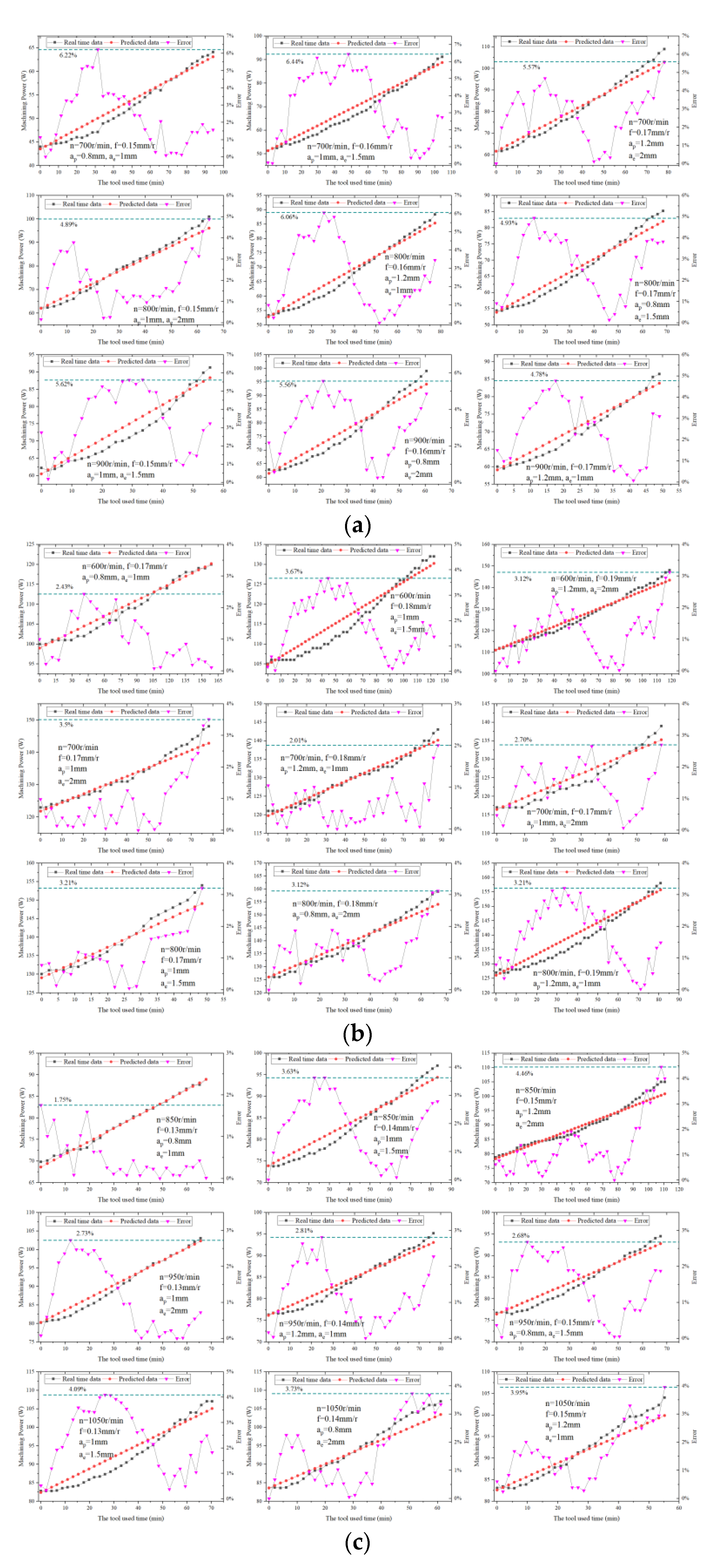
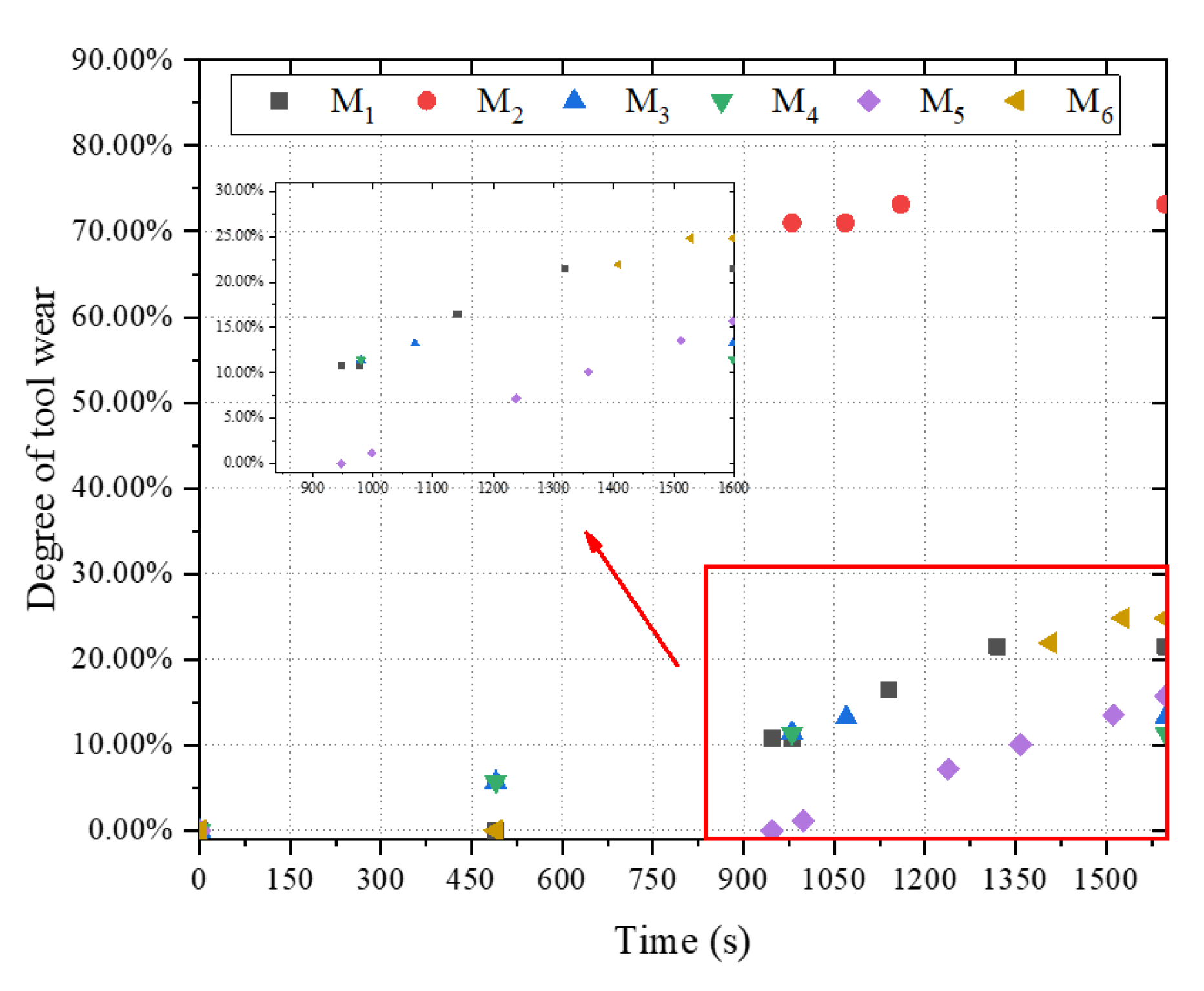
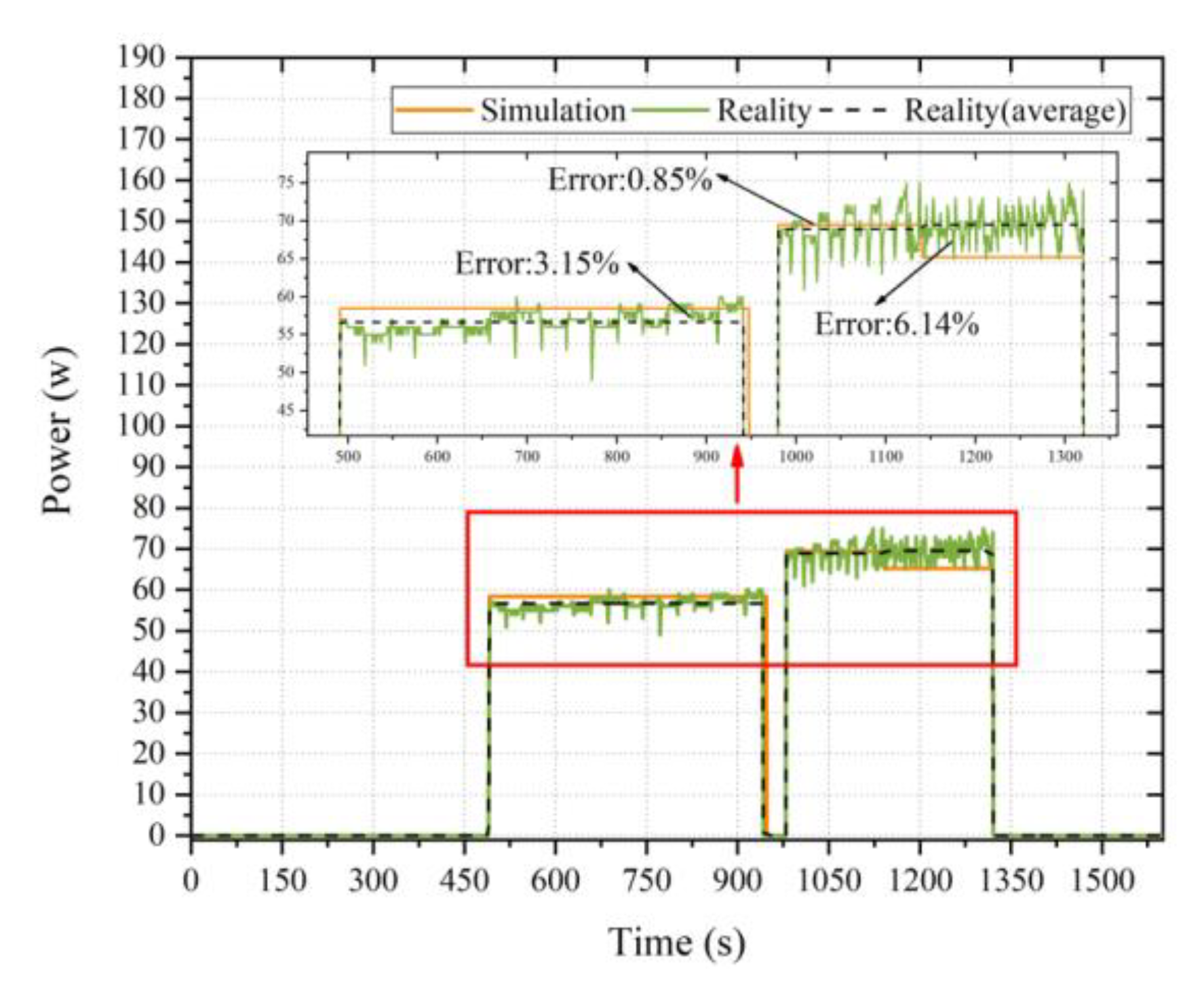
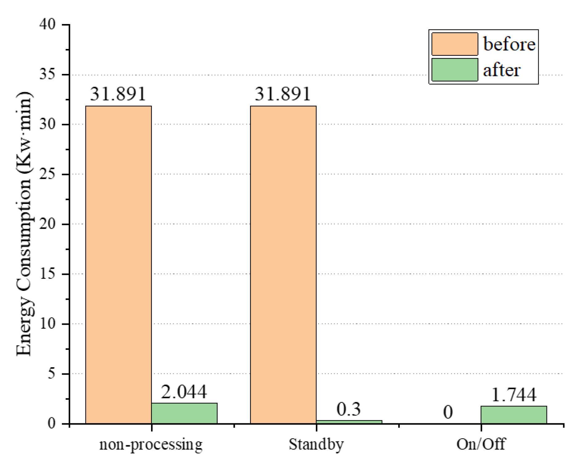
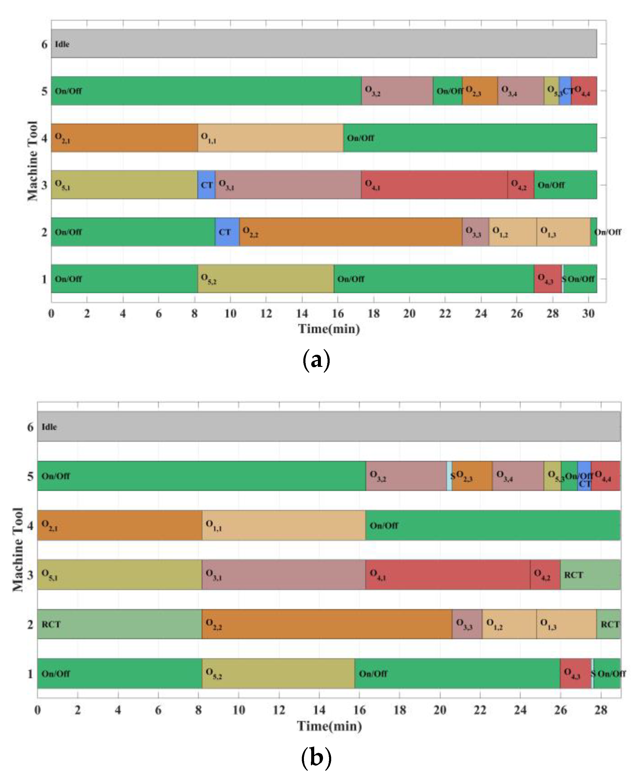
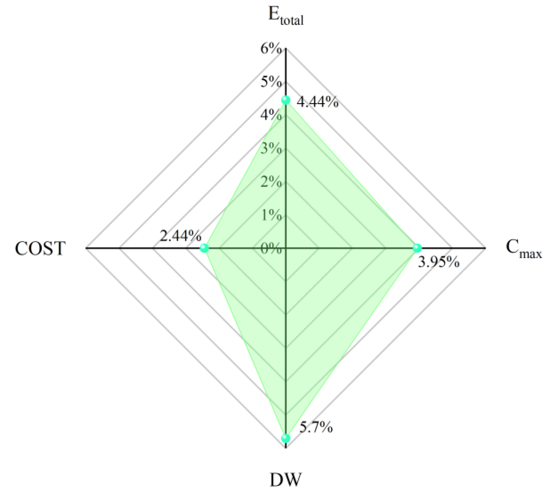
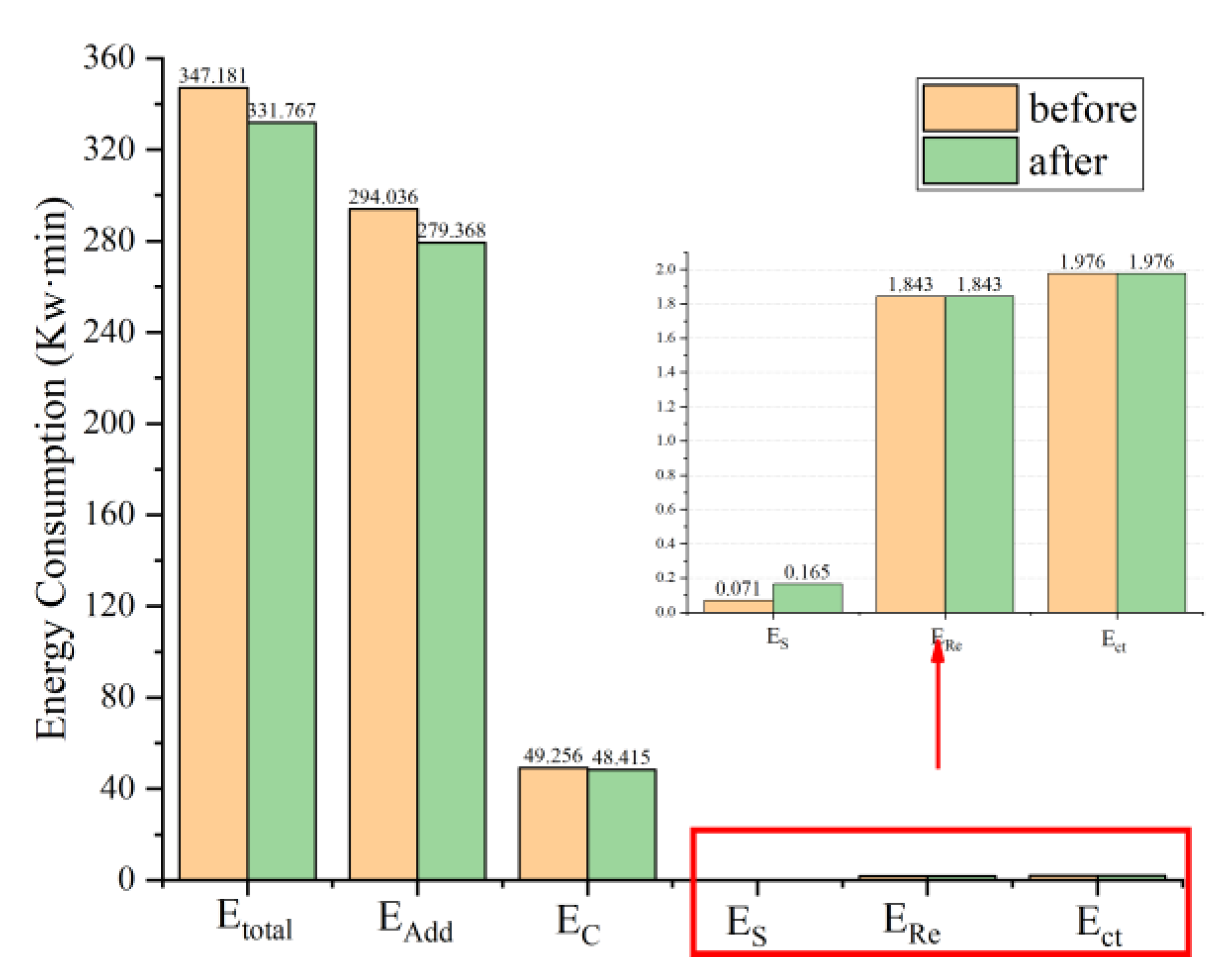
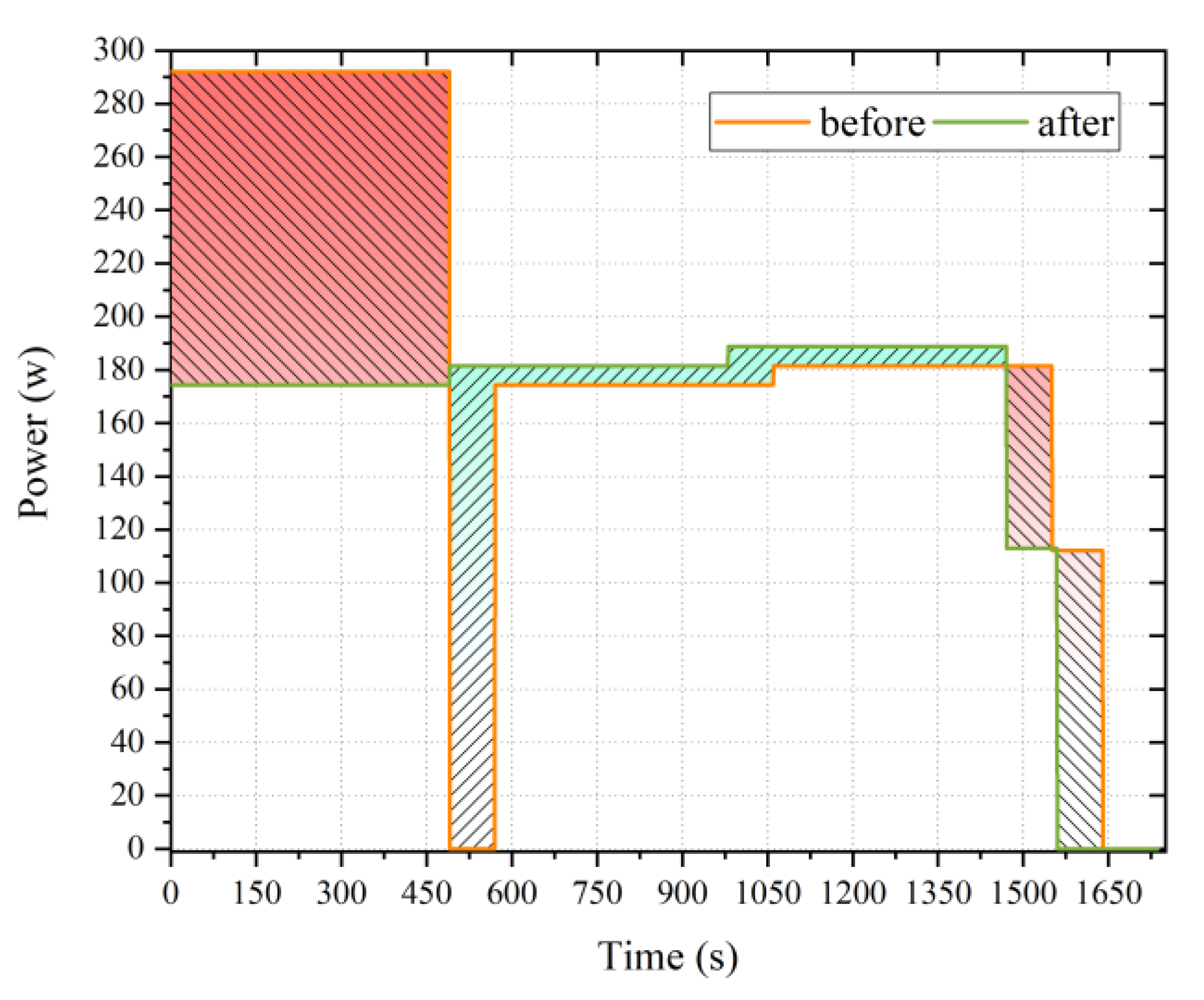
(1) Cutting-tool degradation during shop scheduling was analyzed. Based on the experimental data, exponential regression models of the dynamic power and cutting-tool life were established under certain machining conditions, with an error of approximately 6.5%. (2) A dynamic cutting-tool change strategy by monitoring the RUL was proposed to change the cutting tool before it becomes blunt. This makes the optimization model closer to the real machining situation. (3) Oriented towards low-carbon production objectives, the conventional machine tool turn-on/off schedule can reduce the non-processing energy consumption by 93.5%. Integrating the cutting-tool change strategy into the conventional machine tool turn-on/off schedule further reduces the total energy consumption by 4.44% and production cost by 2.44%. It was proved that this hybrid energy-saving strategy effectively reduces the energy consumption of workshops and has great application prospects.
In terms of the defects in this study, the proposed model does not consider the constraints of transport, clamping, and assembly on shop scheduling. In addition, the establishment of the machining power model and the tool life model of each machine tool in the workshop needs to spend a lot of time on the cutting wear experiment (about 45 h), which brings a lot of work to the preparation of the early production. When the shop changes the machine tool or changes a different type of tool, the models need to be rebuilt. Based on the above limitations, some suggestions are recommended as follows: (1) To explore a fast method to obtain the machining power model and the tool life model and make these models have a certain universal applicability. (2) To integrate more practical constraints such as transport, clamping, assembly, random breakdown or rush orders into the optimization model. (3) To design an efficient solution algorithm to solve multi-objective and many-objective optimization problems.

Author Contributions

Conceptualization, Y.T. and Z.G.; methodology, Y.T. and Z.G.; software, Z.G.; validation, Z.G.; formal analysis, Z.G.; investigation, Y.T., Z.G., L.Z., Y.C. and T.W.; resources, Y.T., L.Z. and T.W.; data curation, Z.G. and Y.C.; writing—original draft preparation, Y.T. and Z.G.; writing—review and editing, Y.T., Z.G. and T.W.; visualization, Z.G.; supervision, Y.T. and Z.G.; project administration, Y.T., L.Z. and Z.G.; funding acquisition, Y.T. All authors have read and agreed to the published version of the manuscript.

Funding

This research was funded by the National Natural Science Foundation of China, grant number 51975407.

Data Availability Statement

Not applicable.

Acknowledgments

The authors would like to thank the editors and anonymous reviewers whose comments helped greatly improve this paper. The work is supported by the National Natural Science Foundation of China (Grant No.51975407).

Conflicts of Interest

The authors declare no conflict of interest.

References

  1. Zhou, L.; Li, J.; Li, F.; Meng, Q.; Li, J.; Xu, X. Energy consumption model and energy efficiency of machine tools: A comprehensive literature review. J. Clean. Prod. 2016, 112, 3721–3734. [Google Scholar] [CrossRef]
  2. Danil, Y.P.; Mozammel, M.; Munish, K.G.; Álisson, R.M.; Giuseppe, P.; Deepak, R.U.; Navneet, K.; Aqib, M.K.; Ítalo, T.; Szymon, W.; et al. Resource saving by optimization and machining environments for sustainable manufacturing: A review and future prospects. Renew. Sustain. Energy Rev. 2022, 166, 112660. [Google Scholar]
  3. Bi, Z.M.; Wang, L.H. Optimization of machining processes from the perspective of energy consumption: A case study. J. Manuf. Syst. 2012, 31, 420–428. [Google Scholar] [CrossRef]
  4. Zeng, L.L.; Zhou, F.X.; Xu, X.H.; Gao, Z. Dynamic scheduling of multi-task for hybrid flow-shop based on energy consumption. In Proceedings of the 2009 International Conference on Information and Automation, Zhuhai/Macau, China, 22–24 June 2009; pp. 478–482. [Google Scholar]
  5. Guzman, E.; Andres, B.; Poler, R. Models and algorithms for production planning, scheduling and sequencing problems: A holistic framework and a systematic review. J. Ind. Inf. Integr. 2022, 27, 100287. [Google Scholar] [CrossRef]
  6. Feng, Y.; Hong, Z.; Li, Z.; Zheng, H.; Tan, J. Integrated intelligent green scheduling of sustainable flexible workshop with edge computing considering uncertain machine state. J. Clean. Prod. 2020, 246, 119070. [Google Scholar] [CrossRef]
  7. Guzman, E.; Andres, B.; Poler, R. Matheuristic algorithm for job-shop scheduling problem using a disjunctive mathematical model. Computers 2021, 11, 1. [Google Scholar] [CrossRef]
  8. Mula, J.; Díaz-Madroñero, M.; Andres, B.; Poler, R.; Sanchis, R. A capacitated lot-sizing model with sequence-dependent setups, parallel machines and bi-part injection moulding. Appl. Math. Model. 2021, 100, 805–820. [Google Scholar] [CrossRef]
  9. Rakovitis, N.; Li, D.; Zhang, N.; Li, J.; Zhang, L.; Xiao, X. Novel approach to energy-efficient flexible job-shop scheduling problems. Energy 2022, 238, 121773. [Google Scholar] [CrossRef]
  10. Mouzon, G.; Yildirim, M.B.; Twomey, J. Operational methods for minimization of energy consumption of manufacturing equipment. Int. J. Prod. Res. 2007, 45, 4247–4271. [Google Scholar] [CrossRef] [Green Version]
  11. Wu, X.; Sun, Y. A green scheduling algorithm for flexible job shop with energy-saving measures. J. Clean. Prod. 2018, 172, 3249–3264. [Google Scholar] [CrossRef]
  12. Gong, G.; Chiong, R.; Deng, Q.; Gong, X.; Lin, W.; Han, W.; Zhang, L. A two-stage memetic algorithm for energy-efficient flexible job shop scheduling by means of decreasing the total number of machine restarts. Swarm Evol. Comput. 2022, 75, 101131. [Google Scholar] [CrossRef]
  13. Cheng, L.; Tang, Q.; Zhang, L.; Meng, K. Mathematical model and enhanced cooperative co-evolutionary algorithm for scheduling energy-efficient manufacturing cell. J. Clean. Prod. 2021, 326, 129248. [Google Scholar] [CrossRef]
  14. An, Y.; Chen, X.; Zhang, J.; Li, Y. A hybrid multi-objective evolutionary algorithm to integrate optimization of the production scheduling and imperfect cutting tool maintenance considering total energy consumption. J. Clean. Prod. 2020, 268, 121540. [Google Scholar] [CrossRef]
  15. Setiawan, A.; Wangsaputra, R.; Martawirya, Y.Y.; Halim, A.H. An FMS Dynamic Production Scheduling Algorithm Considering Cutting Tool Failure and Cutting Tool Life. IOP Conf. Ser. Mater. Sci. Eng. 2016, 114, 012052. [Google Scholar] [CrossRef] [Green Version]
  16. Liu, F.; Wang, L.Q.; Liu, G.J. Content architecture and future trends of energy efficiency research on machining systems. J. Mech. Eng. 2013, 49, 87–94. [Google Scholar] [CrossRef]
  17. He, Y.; Tian, X.; Li, Y.; Wang, S.; John, W. Modeling machining energy consumption including the effect of toolpath. Procedia CIRP 2020, 90, 573–578. [Google Scholar] [CrossRef]
  18. He, Y.; Tian, X.; Li, Y.; Wang, Y.; Wang, Y.; Wang, S. Modeling and analyses of energy consumption for machining features with flexible machining configurations. J. Manuf. Syst. 2022, 62, 463–476. [Google Scholar] [CrossRef]
  19. Shailendra, P.; Girish, K.G.; Srikanta, R. Modelling of Variable Energy Consumption for CNC Machine Tools. Procedia CIRP 2021, 98, 247–251. [Google Scholar]
  20. Haruhiko, S.; Tetsuo, S. Energy Efficiency in Machining Systems Based on Power-Law Model for Specific Energy Consumption. Procedia CIRP 2022, 107, 931–936. [Google Scholar]
  21. Mikołajczyk, T.; Nowicki, K.; Bustillo, A.; Pimenov, D.Y. Predicting tool life in turning operations using neural networks and image processing. Mech. Syst. Signal Process. 2018, 104, 503–513. [Google Scholar] [CrossRef]
  22. Sun, H.; Liu, Y.; Pan, J.; Zhang, J.; Ji, W. Enhancing cutting tool sustainability based on remaining useful life prediction. J. Clean. Prod. 2020, 244, 118794. [Google Scholar] [CrossRef]
  23. Castejón, M.; Alegre, E.; Barreiro, J.; Hernández, L.K. On-line tool wear monitoring using geometric descriptors from digital images. Int. J. Mach. Tools Manuf. 2007, 47, 1847–1853. [Google Scholar] [CrossRef]
  24. Bagga, P.J.; Bajaj, K.S.; Makhesana, M.A.; Patel, K.M. An online tool life prediction system for CNC turning using computer vision techniques. Mater. Today Proc. 2022, 62, 2689–2693. [Google Scholar] [CrossRef]
  25. Shi, K.; Zhang, D.; Liu, N.; Wang, S.; Ren, J.; Wang, S. A novel energy consumption model for milling process considering tool wear progression. J. Clean. Prod. 2018, 184, 152–159. [Google Scholar] [CrossRef]
  26. Zhang, X.; Yu, T.; Dai, Y.; Qu, S.; Zhao, J. Energy consumption considering tool wear and optimization of cutting parameters in micro milling process. Int. J. Mech. Sci. 2020, 178, 105628. [Google Scholar] [CrossRef]
  27. Muhammad, Y.; Syed, J.; Ashfaq, K.; Mushtaq, K. Development and analysis of tool wear and energy consumption maps for turning of titanium alloy (Ti6Al4V). J. Manuf. Process. 2021, 62, 613–622. [Google Scholar]
  28. Tian, C.; Zhou, G.; Zhang, J. Optimization of cutting parameters considering tool wear conditions in low-carbon manufacturing environment. J. Clean. Prod. 2019, 226, 706–719. [Google Scholar] [CrossRef]
  29. Tian, Y.; Shao, W.; Wang, T. Energy Footprint Modeling and Parameter Optimization in Workshop Manufacturing Process. China Mech. Eng. 2021, 33, 1–10. (In Chinese) [Google Scholar]
  30. ISO 8688-2: 1989; Tool Life Testing in Milling-Part 2: End Milling. IX-ISO: Geneva, Switzerland, 1989.
  31. Deb, K.; Pratap, A.; Agarwal, S.; Meyarivan, T. A fast and elitist multiobjective genetic algorithm: NSGA-II. IEEE Trans. Evol. Comput. 2002, 6, 182–197. [Google Scholar] [CrossRef] [Green Version]
  32. Zhang, G.; Gao, L.; Li, P.; Zhang, C. Improved Genetic Algorithm for the Flexible Job-shop Scheduling Problem. J. Mech. Eng. 2009, 45–47, 145–151. [Google Scholar] [CrossRef]
  33. Leng, J.; Gao, X.; Zhu, J. The application of multivariate linear regression forecast model. J. Stat. Decis. 2016, 7, 82–85. (In Chinese) [Google Scholar]
  34. Chu, H.; Dong, K.; Li, R.; Cheng, Q.; Zhang, C.; Huang, K.; Yang, C.; Zheng, Y. Integrated modeling and optimization of production planning and scheduling in hybrid flow shop for order production mode. Comput. Ind. Eng. 2022, 174, 108741. [Google Scholar] [CrossRef]
  35. Ramya, G.; Chandrasekaran, M.; Arulmozhi, P. Optimization of production cost for integrating job shop scheduling with production resources. Mater. Today Proc. 2021, 37, 1839–1844. [Google Scholar] [CrossRef]
Figure 1. Analysis of energy-saving scheduling research status.
Mathematics 11 00324 g001
Figure 2. Energy-saving scheduling research route.
Mathematics 11 00324 g002
Figure 3. Schematic diagram of energy consumption distributions for different running states.
Mathematics 11 00324 g003
Figure 4. Cutting-tool degradation mechanism.
Mathematics 11 00324 g004
Figure 5. Hybrid mechanism algorithm form of cutting-tool change and machine tool turn-on/off.
Mathematics 11 00324 g005
Figure 6. Chromosome encoding process.
Mathematics 11 00324 g006
Figure 7. Scenario 1: (a) Initial Gantt chart; (b) Adjusted Gantt chart.
Mathematics 11 00324 g007
Figure 8. Scenario 2: (a) Initial Gantt chart; (b) Adjusted Gantt chart.
Mathematics 11 00324 g008
Figure 9. Scenario 3: (a) Initial Gantt chart; (b) Adjusted Gantt chart.
Mathematics 11 00324 g009
Figure 10. Scenario 4: (a) Initial Gantt chart; (b) Adjusted Gantt chart.
Mathematics 11 00324 g010
Figure 11. Scenario 5: (a) Initial Gantt chart; (b) Adjusted Gantt chart.
Mathematics 11 00324 g011
Figure 12. Scenario 6: (1) Sufficient machine-off time; (2) Insufficient machine-off time. (a) Initial Gantt chart; (b) Adjusted Gantt chart.
Mathematics 11 00324 g012
Figure 13. Crossover: (a) Crossover of the process chromosome; (b) Crossover of the machine tool chromosome.
Mathematics 11 00324 g013
Figure 14. Mutation: (a) Crossover of the process chromosome; (b) Crossover of the machine tool chromosome.
Mathematics 11 00324 g014
Figure 15. The tool cutting path.
Mathematics 11 00324 g015
Figure 16. Experimental device: (a) Tool wear detection device; (b) Clamp on power logger (PW3360A982-04); (c) Tool wear detection process; (d) Power acquisition wiring diagram; (e) CNC machining center (M1/2,M3/4,M5/6); (f) Positioning device and fixture.
Mathematics 11 00324 g016aMathematics 11 00324 g016b
Figure 17. Partial tool wear detection photos.
Mathematics 11 00324 g017
Figure 18. Multivariate linear regression method.
Mathematics 11 00324 g018
Figure 19. Three-dimensional model drawing of the five workpieces.
Mathematics 11 00324 g019
Figure 20. Comparison of machining power and tool utilization time data: (a) M1,M2; (b) M3,M4; (c) M5,M6.
Mathematics 11 00324 g020
Figure 21. Pareto solutions.
Mathematics 11 00324 g021
Figure 22. Gantt chart of an instance.
Mathematics 11 00324 g022
Figure 23. Gantt chart of scheme 1.
Mathematics 11 00324 g023
Figure 24. Simulation machining power curve.
Mathematics 11 00324 g024
Figure 25. Scatter chart of tool wear.
Mathematics 11 00324 g025
Figure 26. Comparison curve between simulated power and actual machining power.
Mathematics 11 00324 g026
Figure 27. Influence of the machine tool on/off strategy on non-processing energy consumption.
Mathematics 11 00324 g027
Figure 28. Comparison of scheduling schemes before and after the hybrid energy-saving strategy: (a) Before the hybrid energy-saving strategy; (b) After the hybrid energy-saving strategy.
Mathematics 11 00324 g028
Figure 29. Total impact of the hybrid energy-saving strategy.
Mathematics 11 00324 g029
Figure 30. Effect of the hybrid energy-saving strategy on energy consumption.
Mathematics 11 00324 g030
Figure 30. Power contrast curve of M3 after adopting the hybrid energy-saving strategy.
Mathematics 11 00324 g031
Table 1. The symbols used in this paper.
SymbolDescriptions
i , h The index for jobs, i , h = 1 ,   2 , ,   n
j , g The index for operations, j , g = 1 ,   2 ,   ,   m a x { S i , S g }
m The index for machine tools, m = 1 ,   2 ,   , k
r The index for the machine tool’s processing task, r = 1 ,   2 ,   , l m
l m The number of processing tasks for the machine tool M m
S i The number of operations for job J i
n The number of jobs
kThe number of machine tools
J i The i - t h job
o i , j The j - t h operation of the job J i
M m The m - t h machine tool
P m The total power of the machine tool M m
P i j m The power of operation o i , j   which is on the machine tool M m
P d m The dynamic power of the machine tool M m
P s m The static power of the machine tool M m
P c t m The cutting-tool changing power of the machine tool M m
P A d d The additional power of the workshop
a 1 a 8 The exponential parameters between each cutting parameter and the dynamic power
K 1 , K 2 The coefficients of the dynamic power model
b 1 b 4 The exponential parameters between each cutting parameter and the cutting-tool life
K3The coefficients of the tool life model
n v The spindle speed
fThe feed speed
a p The cutting depth
a e The cutting width
t m The used time of the cutting tool of the machine tool M m
T m The cutting-tool life of the machine tool M m
t c t m The cutting-tool changing time of the machine tool M m
P T The processing time of an operation
P T i j The processing time of the operation o i , j
P T i j m The processing time of the operation which is on the machine tool M m
S T i j The start time of the operation o i , j
S T m r The start time of the r - t h processing task of the machine tool M m
C T i j The end time of the operation o i , j
C T m r The end time of the r - t h processing task of the machine tool M m
T R m The no-load balance time of the machine tool
H m The on/off security threshold time of the machine tool M m
R T m e a n The actual average turning-on/off machine tool time
W m The degree of tool wear
E t o t a l The total energy consumption of the workshop
E c The processing energy consumption of machine tools
E R e The energy consumption of turning on/off machine tools
E R e m The energy consumed by a single on/off of the machine tool
E c t The total energy consumption of changing the cutting tool
E s The standby energy consumption of machine tools
E A d d The additional energy consumption of the workshop
R T E m e a n The actual average energy consumption of turning on/off the machine tool
C m a x The makespan
G The total number of turning-on/off machine tools and changing cutting tools
W L The total load of machine tools
C F m The coefficient of cutting tool capacity of the machine tool M m
D W The degree of reduction in processing capacity of the cutting tool
C O S T The production cost
S F m The additional coefficient of turning on/off the machine tool M m
ω e Unit energy cost
ω m The unit operating cost of the machine tool
ω t Machine tool turn on/off loss cost
ω l Cost per unit of labor time
x The number of tasks that cutting-tool changing operation can be advanced
γ i j m r / γ h g m r γ i j m r / γ h g m r = 1, if the operation o i , j is the r - t h processing task of M m , γ i j m r =1; otherwise γ i j m r / γ h g m r = 0  
η m r η m r = 1, if the machine tool M m is turned on/off before its r - t h processing task; otherwise, η m r = 0
λ m r λ m r = 1, if the machine tool M m changes the cutting tool before its r - t h processing task; otherwise, λ m r = 0
δ m δ m = 1, if the machine tool M m turns on/off twice or more; otherwise, δ m = 0
Table 2. Basic parameters of experimental devices.
Machine ToolsMachine Tools Type (Model)Cutting-Tool TypeDiameter of Milling Cutter Edge (mm)Milling Cutter MaterialNumber of Milling Cutter EdgesLength of Milling Cutter Edge (mm)Length of Milling Cutter (mm)Cutting FluidAnti-wear Coating
M 1 , M 2 Three-axis CNC machining center(TSIM-VMA8050V4)End Millφ10M2AI high-speed steel42566WaterNo
M 3 , M 4 Three-axis CNC machining center (TSIM-VMC1580)End Millφ12M2AI high-speed steel43585WaterNo
M 5 , M 6 Five-axis CNC machining center (TSIM-VMA210V)End MillΦ8M2AI high-speed steel42266WaterNo
Table 3. Experimental cutting parameters table.
Machine Tools n v   ( r / m i n ) f   ( m m / r ) a p   ( m m ) a e   ( m m )
M 1 , M 2 7000.150.81
0.1611.5
0.171.22
8000.1512
0.161.21
0.170.81.5
9000.1511.5
0.160.82
0.171.21
M 3 , M 4 6000.170.81
0.1811.5
0.191.22
7000.1712
0.181.21
0.190.81.5
8000.1711.5
0.180.82
0.191.21
M 5 , M 6 8500.130.81
0.1411.5
0.151.22
9500.1312
0.141.21
0.150.81.5
10500.1311.5
0.140.82
0.151.21
Table 4. Cutting-tool degradation model.
Machine ToolsModel
M 1 , M 2 P d = 0.9442 n v 0.6385 f 0.1416 a p 0.3255 a e 0.2693 + 4.24 × 10 5 t m n v 1.6716 f 1.2510 a p 0.9296 a e 0.7356
T = 10.0048 n v 0.3821 f 2.44733 a p 0.59782 a e 0.26984
M 3 , M 4 P d = 1.0400 n v 0.6580 f 0.2245 a p 0.1842 a e 0.0789 + 2.24 × 10 5 t m n 2.2058 f 3.0474 a p 0.0977 a e 0.4933
T = 23.3873 n v 0.1448 f 1.2645 a p 0.7309 a e 0.0774
M 5 , M 6 P d = 1.7413 n v 0.5870 f 0.1269 a p 0.1231 a e 0.0932 + 1.15 × 10 5 t m n v 0.3816 f 2.5387 a p 0.5164 a e 0.2689
T = 25.5911 n v 0.1248 f 0.0842 a p 0.0048 a e 0.0726
Table 5. Machine tool information.
Machine Tools The   No-Load   Balance   Time   ( T R m / s ) The   on / off   Sec urity   Threshold   Time   ( H k / s ) Cutting-Tool   Change   Time   ( t c t / s ) / Power   ( P c t / W ) Static   Power   ( P s m / W )
M 1 , M 2 4810060/195520
M 3 , M 4 459080/295420
M 5 , M 6 326040/156325
Table 6. Workpiece information.
Job NumberOperationsOptional Machine ToolsProcessing Time (min) Cutting   Parameters   ( n v ,   f ,   a p ,   a e )
J 1 O 1 , 1 Milling 50 × 50 × 15 convex platform M 1 , M 2 16.34900,0.17,3,2.5
M 3 , M 4 8.16800,0.19,3,5
O 1 , 2 Milling 30 × 10 × 15 slot M 1 , M 2 2.68700,0.16,1.5,2
O 1 , 3 Enlarge holes 2 × 12 × 15   2 × 15 × 15 M 1 , M 2 3700,0.15,1.5,1.5
M 5 , M 6 4850,0.13,1.5,1.5
J 2 O 2 , 1 Milling 50 × 50 × 15 convex platform M 1 , M 2 16.34900,0.17,3,2.5
M 3 , M 4 8.16800,0.19,3,5
O 2 , 2 Milling 40 × 40 × 10 convex platform M 1 , M 2 12.45900,0.15,2.5,2.5
M 5 , M 6 14.81050,0.13,2,2.5
O 2 , 3 Enlarge hole 12 × 15   15 × 15 M 5 , M 6 2850,0.13,1.5,1.5
J 3 O 3 , 1 Milling 50 × 50 × 15 convex platform M 1 , M 2 16.34900,0.17,3,2.5
M 3 , M 4 8.16800,0.19,3,5
O 3 , 2 Milling 2 × 27 × 8 × 8 slots M 5 , M 6 4850,0.13,1,2
O 3 , 3 Enlarge hole 12 × 15   15 × 15 M 1 , M 2 1.5700,0.15,1.5,1.5
M 5 , M 6 2850,0.13,1.5,1.5
O 3 , 4 Enlarge holes 2 × 10 × 15   2 × 11 × 15 M 5 , M 6 2.56850,0.13,1,0.5
J 4 O 4 , 1 Milling 50 × 50 × 15 convex platform M 1 , M 2 16.34900,0.17,3,2.5
M 3 , M 4 8.16800,0.19,3,5
O 4 , 2 Milling 19 × 12 × 8 slot M 3 , M 4 1.49600,0.17,1,2
O 4 , 3 Milling 2 × 10 × 10 × 8 slots M 1 , M 2 1.53700,0.15,1,2
O 4 , 4 Milling 2 × 10 × × 8 × 8 slots M 5 , M 6 1.45850,0.13,1,2
J 5 O 5 , 1 Milling 50 × 50 × 15 convex platform M 1 , M 2 16.34900,0.17,3,2.5
M 3 , M 4 8.16800,0.19,3,5
O 5 , 2 Milling 2 × 50 × 10 × 8 slots M 1 , M 2 7.62700,0.15,1,2
O 5 , 3 Enlarge hole 9 × 15   10 × 15 M 5 , M 6 0.85850,0.13,1,0.5
Table 7. Related unit costs.
Unit Energy Cost (CNY/KW·h)Unit Operating Cost of Machine Tool (CNY/h)Machine Tool Turn on/off Loss Cost (CNY/time)Cost Per Unit of Labor Time (CNY/h)
0.725 9130
Table 8. Cutting-tool degradation model.
Pareto Numbers Pareto   Solutions   ( C m a x ( min ) , E t o t a l ( K w · m i n ) ,   W L ( min ) , G (time)) Production Cost (CNY)
15(29.60,337.46,81.93,7), (28.95,329.10,84.78,8), (27.18,319.5,90.61,8), (28.95,331.36,81.93,8),(28.95,331.32,82.43,9), (27.18,317.67,92.96,8), (28.95,329.10,84.78,8), (28.95,329.34,84.28,9),(28.96,329.01,85.78,8), (28.95,331.36,81.93,8), (27.79,325.47,90.11,8), (28.96,334.26,93.96,7),
(29.47,335.72,82.43,6), (31.18,349.53,85.78,5), (29.60,334.64,85.78,6)
37.17, 38.17, 38.04, 37.77, 38.84, 38.37, 38.17, 39.10, 38.32, 37.77, 38.34, 38.61, 36.16, 36.68, 36.71
Disclaimer/Publisher’s Note: The statements, opinions and data contained in all publications are solely those of the individual author(s) and contributor(s) and not of MDPI and/or the editor(s). MDPI and/or the editor(s) disclaim responsibility for any injury to people or property resulting from any ideas, methods, instructions or products referred to in the content.

