Asymptotic Study of Longitudinal Velocity Influence and Nonlinear Elastic Characteristics of the Oscillating Moving Beam

Abstract

Mathematical models of the nonlinear transversal oscillations for a beam moving along its axis have been studied. These models deal with the nonlinearity of body elastic properties and with the influence of physical–mechanical and kinematic parameters on the oscillation amplitude and frequency of the moving one-dimensional nonlinear systems as well. A procedure for studying both cases, non-resonance and resonance oscillation regimes, has been developed. The paper focuses on the influence of the longitudinal velocity, nonlinear elastic material properties, and external periodical perturbations on the dynamical process of beam transversal oscillation. The obtained mathematical model could be applied to describe the oscillation behavior of the different types of pipelines (liquid or gas). The proposed results allow the estimation of the influence of these parameters on the amplitude and frequency of the oscillations. Mathematical analysis realized by asymptotic methods enables the prediction of the resonance phenomena and proposal of a numerical algorithm to plan the most effective operation regime. Applications of this approach in engineering, particularly to construct the corresponding elements of industrial environments and pipelines, are also discussed.

1. Introduction

It is common knowledge [1,2,3,4] that the transverse vibrations of a beam moving along its axis are widely used in industry, technological processes, construction, etc. For example, it is important to study the telescopic boom of a crane [3]. Models of axially moving materials can be used in the field of automotive and aerospace structures, in mathematical models of robot motion, etc. The equation of motion is the same for the vibration of a pipeline with liquid or gas flowing through it [5,6]. In all the above cases, as well as in some other mathematical models of vibrations, the equation of motion is a weakly nonlinear equation of the hyperbolic type. Asymptotic methods of nonlinear mechanics are effectively used to study such nonlinear systems with distributed parameters when describing single-frequency vibration modes [7,8]. For these systems, the perturbed nonlinear boundary problem with single-frequency vibration is solved (in the first approximation) by asymptotic expansion in the form of corresponding normal vibrations of the unperturbed system. At the same time, amplitudes and phases are time-varying quantities. For engineering calculations, it is sufficient to know the influence of the speed, disturbing force, and the values of the physical and mechanical characteristics of the material (density, modulus of elasticity, mass, etc.) of the beam on the law of change in the amplitude and the phase of transverse vibrations [9,10,11]. According to the asymptotic method, such influences on the amplitude–frequency characteristics of vibrations are determined from the system of ordinary differential equations for self-vibrating systems and, in the non-resonant case, for non-autonomous systems.

This approach is quite effective for the study of the dynamic processes of one-dimensional systems, which are described by partial differential equations. Depending on the method of fixing the medium, the boundary conditions can be divided into homogeneous (when the ends are rigidly fixed and stationary) and non-homogeneous (when the ends vibrate or can be affected by forces, moments, etc.) [12].

The subject of study in this article is the influence of the following parameters of the dynamic process on the amplitude and phase characteristics (APC) of the dynamic process during transverse vibrations of the beam: the longitudinal speed of the beam, nonlinear elastic characteristics of its material, and external periodic disturbances. The research is based on the principle of single-frequency vibrations in nonlinear systems with many degrees of freedom and distributed parameters and the asymptotic method of solving certain classes of differential equations with partial derivatives.

In [13], free transverse vibrations of beam-type bodies with a variable cross-section were investigated using the Wentzel, Kramers, and Brillouin (WKB) approximation. The authors obtained mathematical models that were used to determine natural frequencies and forms of modes. Several examples of vibrating systems of the beam type with and without a distributed axial force were given.

In [14], the dynamics of a hyperelastic beam in a curved state affected by a harmonic axial load is investigated. For the static case, the curved configuration of the hyperelastic beam is first determined using the asymptotic method when the axial load exceeds the critical load. The amplitude–frequency characteristics of a hyperelastic curved beam are obtained using the Runge–Kutta method and the harmonic balance method. The authors numerically investigated the effect of the external average axial load, the amplitude of the axial load change, and geometric and physical parameters on the amplitude–frequency characteristics of the curved beam.

In [15], the asymptotic method was used to study the free vibrations of heterogeneous beams with different boundary conditions.

A new theoretical approach to the characterization of transverse vibrations of cantilever beams under the effect of a continuous spatially distributed load was proposed in [16]. Despite certain limitations (time-independent load, homogeneous boundary conditions), the obtained result is quite general and applicable to a wide class of spatially dependent loads.

In [17], a frequency equation of the transverse vibrations of a non-uniform and non-homogeneous beam was derived using asymptotic approximation. The authors obtained a mathematical model that is simple and accurate enough to determine the frequency of vibration, but also general enough to be used in engineering calculations. In these materials, the asymptotic perturbation approach (APA) is applied to obtain a simple analytical expression for the analysis of free vibrations of non-uniform and non-homogeneous beams with different boundary conditions.

Free vibrations of a two-layer beam were studied. Asymptotic approximation was used to estimate when axial and rotational inertia and shear deformations, and the normal compliance of the interface could be neglected [18].

In [19], a nonlinear algebraic system was solved with the help of the asymptotic method, which was used for the main vibration mode of a nonlinear beam loaded with a finite number of masses. The method was based on Hamilton’s principle and spectral analysis for nonlinear free vibrations that show large displacement amplitudes. The problem is reduced to solving a nonlinear algebraic system by numerical or analytical methods.

Numerous studies [20] were performed to analyze the transverse vibrations of elastic beams loaded with a finite number of point masses at a limited position of the beam with only one or two boundary conditions. Most of these studies were presented without considering the effect of inertial forces in beams.

In [21], the linear dynamics of an elastic beam consisting of three linear–elastic isotropic layers was studied using asymptotic expansion.

The study most similar to ours was carried out in [22], where the numerical analysis of jump-like sliding vibrations of a beam moving in the transverse direction is presented. The effect of axial load and motion speed on the dynamic response is also studied.

Paper [23] considered the eigen-frequencies and dynamic characteristics of a thick beam composed of saturated porous materials resting on a viscoelastic foundation. The authors’ obtained results show that, under some conditions, the beam has the smallest fundamental frequency, and when increasing the Skempton coefficient, the fundamental frequency of the beam also increases. Our study deals with another mathematical model describing thin beam oscillations.

In [24], the nonlinear transverse vibration of an axially accelerating moving viscoelastic sandwich beam with time-dependent tension has been analyzed. Numerical results that show the influence of the initial tension and phase angle effect on the natural frequencies and response curves are presented.

Paper [25] described the free oscillation behavior of multi-layer composite beams reinforced with graphene platelets with a viscoelastic foundation. The main issue of the paper concentrated on the graphene platelets’ material characteristics. All parameter effects on the oscillations were studied thoroughly.

It is useful to notice that, as considered in this paper, differential equations can be applied in other scientific fields as well (chemistry, biology, etc.). They describe the oscillations of chemical reactions [26]. The modeling of such types of reactions depends on the choice of the velocity values and the initial and boundary conditions.

However, in all the aforementioned studies of beam vibrations, the influence of its longitudinal velocity was not taken into account, and in [22], the authors only tried to consider a similar problem and did not obtain mathematical models for nonlinear–elastic one-dimensional systems in a general form.

A specific feature of our study is the possibility to take into account the influence of the longitudinal velocity, elasticity modulus, material density, and beam length on the amplitude–frequency characteristics of the transversal oscillations. It enables us to establish more exactly the oscillation amplitude for nonlinear elastic moving systems in the resonance and non-resonance cases as well. This is why the use of simple calculation formulae for the description of amplitude change laws is reasonable.

2. Materials and Methods

2.1. Mathematical Models of Transverse Vibrations of a Moving Beam under Homogeneous Boundary Conditions

Let us consider the transverse vibrations of a beam moving along an undeformed axis at a constant speed (Figure 1). The following conditions are assumed: (а) the material of the beam satisfies a law of elasticity close to the linear one; (b) external periodic disturbances act on the beam; (c) the beam is moving along its geometric axis at a constant speed.

The following notations are used in Figure 1:

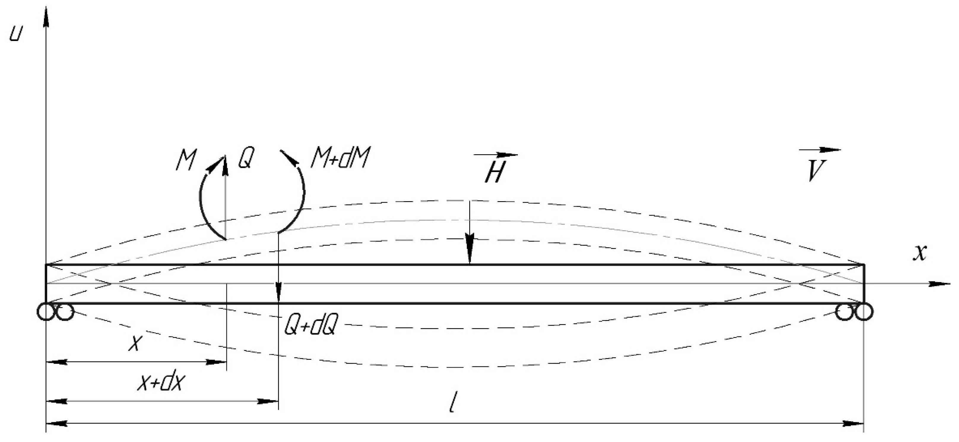
• M is the torque acting on the beam element with coordinate x;
• Q is the force acting on the beam element with coordinate x;
• M + dM is the torque acting on the beam element with coordinate х + dx;
• Q + dQ is the force acting on the beam element with coordinate х + dx;
• H is the harmonic force acting on the beam with its own amplitude and frequency;
• l is the beam length;
• V is the longitudinal speed of a beam moving along its axis.

To describe transverse vibrations, we will take the rectilinear axis x as the coordinate axis, and from it we will calculate the deviation of the beam elements during transverse vibrations. Let us assume the following:

• Deviations of individual points of the axis of the beam are perpendicular to its rectilinear, undeformed direction. At the same time, the displacement of these points parallel to the axis Ox is neglected;
• Deviations of the points of the beam axis for transverse vibrations occur in one plane (“in the plane of vibrations”);
• The cross-section of the beam is always perpendicular to the axis—that is, it does not undergo deplenation [27].

Under such assumptions, the deviations of the beam axis points during transverse vibrations are uniquely determined by one function of two variables—the coordinate х and the time $t$. Let us denote such a function by $u=u\left(x,t\right)$, which is the function that determines the position of a point with the coordinate $x$ at any moment of time $t$.

Let us also introduce the following denotations:

• m(x) is the mass of a unit of the beam length;
• E is the modulus of elasticity of the first kind (Young’s modulus);
• I is the moment of inertia of the cross-section of the beam relative to the neutral axis of the section, which is perpendicular to the vibration plane.

The mathematical model that we consider uses the Euler–Bernoulli beam theory. This is due to the fact that the deformations of the beam are small and are under a transverse load.

Then, the differential equation of transverse vibrations of the beam has the following form [7,28]:

$$\frac{d^{2}u}{d{t}^2}+{\alpha }^2\frac{{\partial }^{4}u}{\partial x^4}=\epsilon F\left(u,\theta ,\frac{\partial u}{\partial t},\frac{\partial u}{\partial x},\frac{{\partial }^{2}u}{\partial x^2},\frac{{\partial }^{3}u}{\partial x^3},\frac{{\partial }^{4}u}{\partial x^4}\right)$$

(1)

where ${\alpha }^2=\frac{EI}{m}$; $\epsilon$ is a small positive parameter; $\theta$ is the phase of vibrations of the harmonic force acting on the beam; $\frac{d\theta }{dt}=\nu \left(t\right)$ is a positive function (instantaneous frequency of disturbance force fluctuations); $F\left(u,\theta ,\frac{\partial u}{\partial t},\frac{\partial u}{\partial x},\frac{{\partial }^{2}u}{\partial x^2},\frac{{\partial }^{3}u}{\partial x^3},\frac{{\partial }^{4}u}{\partial x^4}\right)$ is analytical $2\pi$ periodic to the $\nu t=\theta$ function that is infinitely differentiated by all its arguments. It is necessary to present $F\left(u,\theta ,\frac{\partial u}{\partial t},\frac{\partial u}{\partial x},\frac{{\partial }^{2}u}{\partial x^2},\frac{{\partial }^{3}u}{\partial x^3},\frac{{\partial }^{4}u}{\partial x^4}\right)$ below as a Fourier series. According to [25,26], it can be presented as follows:

$$F\left(u,\theta ,\frac{\partial u}{\partial t},\frac{\partial u}{\partial x},\frac{{\partial }^{2}u}{\partial x^2},\frac{{\partial }^{3}u}{\partial x^3},\frac{{\partial }^{4}u}{\partial x^4}\right)={{\displaystyle \sum }}_{n=-N}^N{e}^{in\nu t}{F}_n\left(u,\frac{\partial u}{\partial t},\frac{\partial u}{\partial x},\frac{{\partial }^{2}u}{\partial x^2},\frac{{\partial }^{3}u}{\partial x^3},\frac{{\partial }^{4}u}{\partial x^4}\right)$$

(2)

where $F_n\left(u,\frac{\partial u}{\partial t},\frac{\partial u}{\partial x},\frac{{\partial }^{2}u}{\partial x^2},\frac{{\partial }^{3}u}{\partial x^3},\frac{{\partial }^{4}u}{\partial x^4}\right)$ are the values of the function $F\left(u,\theta ,\frac{\partial u}{\partial t},\frac{\partial u}{\partial x},\frac{{\partial }^{2}u}{\partial x^2},\frac{{\partial }^{3}u}{\partial x^3},\frac{{\partial }^{4}u}{\partial x^4}\right)$ in points (n = 0, ±1, ±2, ±3...). Moreover, we need to calculate the horizontal speed of the beam. For this purpose, let us write the following:

$$\frac{d}{dt}=\frac{\partial }{\partial x}\frac{dx}{dt}+\frac{\partial }{\partial t}=V\frac{\partial }{\partial x}+\frac{\partial }{\partial t},$$

(3)

$$\frac{d^2}{d{t}^2}=\frac{{\partial }^2}{\partial x^2}{\left(\frac{dx}{dt}\right)}^2+2\frac{dx}{dt}\frac{{\partial }^2}{\partial x\partial t}+\frac{{\partial }^2}{\partial t^2}=V^2\frac{{\partial }^2}{\partial x^2}+2V\frac{{\partial }^2}{\partial x\partial t}+\frac{{\partial }^2}{\partial t^2}.$$

(4)

At the same time, let us assume that the coefficients $F_n\left(u,\frac{\partial u}{\partial t},\frac{\partial u}{\partial x},\frac{{\partial }^{2}u}{\partial x^2},\frac{{\partial }^{3}u}{\partial x^3},\frac{{\partial }^{4}u}{\partial x^4}\right)$ in the right-hand part of (2) are certain polynomials relative to $\frac{\partial u}{\partial t},\frac{\partial u}{\partial x},\frac{{\partial }^{2}u}{\partial x^2},\frac{{\partial }^{3}u}{\partial x^3},\frac{{\partial }^{4}u}{\partial x^4}$ [7].

The beam moves along its axis with a constant speed; therefore, considering the movement of the medium (3) and (4), Equation (1) acquires the following form:

$$\frac{{\partial }^{2}u}{\partial t^2}+{\alpha }^2\frac{{\partial }^{4}u}{\partial x^4}+2V\frac{{\partial }^{2}u}{\partial x\partial t}+V^2\frac{{\partial }^{2}u}{\partial x^2}=\epsilon F\left(u,\theta ,\frac{\partial u}{\partial t},\frac{{\partial }^{2}u}{\partial x^2},\dots ,\frac{{\partial }^{4}u}{\partial x^4}\right)$$

(5)

The function $F\left(u,\theta ,\frac{\partial u}{\partial t},\frac{\partial u}{\partial x},\frac{{\partial }^{2}u}{\partial x^2},\frac{{\partial }^{3}u}{\partial x^3},\frac{{\partial }^{4}u}{\partial x^4}\right)$ takes into account the nonlinear elastic features of the medium as well as dissipative and resistance forces if such forces are small in comparison with nonlinear elastic forces and external periodic disturbances.

For Equation (5), we shall consider boundary conditions that correspond to the imperfect hinged fastening of the ends of the beam [1,6]—that is,

$$u{\left(x,t\right)|}_{x=0}^{x=l}=\epsilon p_j{\left(\theta ,u\right)|}_{x=0}^{x=l},{\frac{{\partial }^{2}u}{\partial x^2}\left(x,t\right)|}_{x=0}^{x=l}=\epsilon r_j{\left(\theta ,\frac{\partial u}{\partial t}\right)|}_{x=0}^{x=l}\mathrm{at}j=0,l,$$

(6)

where $p_j\left(\theta ,u\right),r_j\left(\theta ,\frac{\partial u}{\partial t}\right)$ is a nonlinear function relative to $u,\frac{\partial u}{\partial t}$ and quite smooth relative to their arguments. In practice, the following methods of beam fastening are possible [12]:

-

the end of the rod is free, and at this end the bending moment and the transverse force are equal to zero: $\frac{{\partial }^{2}u}{\partial t^2}=0$, $\frac{{\partial }^{3}u}{\partial t^3}=0$ at $x=l$;

-

the end of the rod is rigidly fixed, while the deflection and the rotation angle are equal to zero: $u=0$, $\frac{\partial u}{\partial t}=0$ at $x=l$;

-

the end of the rod is freely supported or hinged; then, the deflection and the bending moment are also zero: $u=0$, $\frac{{\partial }^{3}u}{\partial t^3}=0$ at $x=l$.

When studying the transverse vibrations of the beam, we will assume that the speed of longitudinal movement is small. Such a limitation allows the asymptotic method of nonlinear mechanics to be applied to the study of vibrations [28].

According to this approach, we will search for the solution of Equation (5) in the first approximation in the following form:

$$u\left(x,t\right)=a{X}_k\left(x\right)T(\psi ,\theta )+\epsilon u_1\left(a,\psi ,\theta ,x\right)$$

(7)

where a is the amplitude of single-frequency vibrations; $u_1\left(a,\psi ,\theta ,x\right)$ is a function periodical by $\psi$ and $\theta$ with the period $2\pi$; $\psi$ is the phase of transverse vibrations of the beam; $\frac{d\psi }{dt}=\omega$ is a positive function (frequency of natural vibrations of the beam); $T\left(\psi ,\theta \right)=\cos \left(\omega t-\theta \right)$; $X_k\left(x\right)$ is a function that determines the shape of the vibrations and can take the following form:

(a)

during vibrations of a homogeneous beam fixed at points with coordinates 0 and l,

$$X_k\left(x\right)=\sin \frac{k\pi x}{l},k=1,2,\dots ,$$

(8)

that is, this form of the function allows for movement and will have the appearance of a fixed hinge type [29,30];

(b)

during vibrations of a homogeneous beam, which is immovably fixed at one end, and its other end is free $X_k\left(x\right)=C\left[U\left(kx\right)-\frac{V\left(kl\right)}{S\left(kl\right)}V\left(kx\right)\right]$, where С is a certain constant, which is selected in such a way that the resulting expression at certain t should not go beyond the sign of sine or cosine, $V\left(x\right)$ and $S\left(x\right)$ is Krylov’s function, $V\left(x\right)=\frac{1}{2}\left(shkx-\sin kx\right)$, $S\left(x\right)=\frac{1}{2}\left(chkx+\cos kx\right)$ and $U\left(x\right)=\frac{1}{2}\left(chkx-\cos kx\right)$;

(c)

during vibrations of a homogeneous beam, the ends of which are immovably fixed $X_k\left(x\right)=C\left[U\left(kx\right)-\frac{T\left(kl\right)}{U\left(kl\right)}V\left(kx\right)\right]$, $T\left(x\right)$ is Krylov’s function, $T\left(x\right)=\frac{1}{2}\left(shkx+\sin kx\right)$;

(d)

during vibrations of a homogeneous beam with free ends $X_k\left(x\right)=A\left[S\left(kx\right)-\frac{T\left(kl\right)}{U\left(kl\right)}T\left(kx\right)\right]$, А is a certain constant, which is selected in such a way that the resulting expression at certain $t$ should not go beyond the sign of sine or cosine;

(e)

during vibrations of a homogeneous beam, one end of which is rigidly fixed and the other one is hinged, $X_k\left(x\right)=C\left[U\left(kx\right)-\frac{S\left(kl\right)}{T\left(kl\right)}V\left(kx\right)\right]$.

Let us focus on the simplest case, when the ends of the beam are hinged but allow transverse movements. Taking into account that the studied system is subject to periodic disturbances, two cases should be considered for its study: non-resonant—$\omega \ne \nu$ and resonant—$\omega \approx \nu$ (in our investigation, we shall focus on the case of the main resonance). As for longitudinal vibrations, the magnitude of the frequency of the disturbing force has a significant effect on the APC.

2.2. Non-Resonant Case of Vibrations

In contrast to the linear case, the parameters $a$ and $\psi$ will be variable and in representation (7) will take into account the influence of nonlinear, periodic forces, as well as the effect of the moving environment on the APC of the dynamic process. As in [7,9], we will set the laws of change in the specified parameters using differential equations:

$$\begin{gathered} \frac{da}{dt}=\epsilon A_1\left(a\right)+\dots \\ \frac{d\psi }{dt}=\omega +\epsilon B_1\left(a\right)+\dots \end{gathered}$$

(9)

while finding the functions $A_1\left(a\right)$ and $B_1\left(a\right)$ in such a way as in Equation (7), in which we substitute the derivatives (9) instead of $a\left(t\right)$ and $\psi \left(t\right)$, and they should satisfy the boundary conditions (6) with the required degree of accuracy.

Therefore, the task of constructing an approximate solution of the system of Equation (9) consists in finding the functions $A_1\left(a\right)$, $B_1\left(a\right)$ and $u_1$(a, $\psi$, $\theta$, x). For this, let us differentiate the dependence (7) taking into account (8). For the first approximation, the following is received:

$$\begin{gathered} \frac{\partial u}{\partial t}=\epsilon A_1\left(a\right)X_k\left(x\right)\cos \psi -a{X}_k\left(x\right)\left(\sin \psi \left(\omega +\epsilon B_1\left(a\right)\right)\right) \\ +\frac{\partial u_1}{\partial \psi }\left(\omega +\epsilon B_1\left(a\right)\right), \end{gathered}$$

(10)

$$\begin{gathered} \frac{{\partial }^{2}u}{\partial t^2}=-a{\omega }^2{X}_k\left(x\right)\cos \psi -2\epsilon a{A}_1\left(a\right)X_k\left(x\right)\sin \psi \\ -2a{B}_1\left(a\right)\omega X_k\left(x\right)\cos \psi +\frac{{\partial }^{2}u}{\partial {\psi }^2}{\omega }^2, \end{gathered}$$

(11)

$$\begin{gathered} \frac{\partial u}{\partial x}=a{X}_k^{\prime }\left(x\right)\cos \psi +\epsilon \frac{\partial u_1}{\partial x},\frac{{\partial }^{2}u}{\partial x^2}=a{X}_k^{″}\left(x\right)\cos \psi +\epsilon \frac{{\partial }^2{u}_1}{\partial x^2}, \\ \frac{{\partial }^{3}u}{\partial x^3}=a{X}_k^{‴}\left(x\right)\cos \psi +\epsilon \frac{{\partial }^3{u}_1}{\partial x^3},\frac{{\partial }^{4}u}{\partial x^4}=a{X}_k^{⁗}\left(x\right)\cos \psi +\epsilon \frac{{\partial }^4{u}_1}{\partial x^4} \end{gathered}$$

(12)

Given these ratios, let us write the general representation for the first approximation:

$$\begin{gathered} \frac{{\partial }^2{u}_1}{\partial {\psi }^2}{\omega }^2+{\alpha }^2\frac{{\partial }^4{u}_1}{\partial x^4}=2a\omega A_1\left(a\right)X_k\left(x\right)\sin \psi \\ +2\omega a{B}_1\left(a\right)X_k\left(x\right)\cos \psi +V^{2}a{X^{″}}_k\left(x\right)\cos \psi +2Va\omega {X^{\prime }}_k\left(x\right)\sin \psi +F\left(a,\psi ,x\right). \end{gathered}$$

(13)

Then, the function $F\left(a,\psi ,x\right)$ will acquire the following form for the case under consideration:

$$F\left(a,\psi ,x\right)=f\left(a\sin \frac{k\pi }{l}x\cos \psi ,a\frac{k\pi }{l}\cos \frac{k\pi }{l}x\cos \psi \right)$$

(14)

To determine the unknown functions A₁(a), B₁(a), let us impose an additional condition on $u_1\left(a,\psi ,x\right)$, similarly to [7]. This condition is the absence of summands proportional to $\sin \frac{k\pi }{l}x\cos \psi$ and $\sin \frac{k\pi }{l}\sin \psi$ in its expansion. This allows us to obtain the aforesaid functions in the following form:

$$\begin{gathered} A_1\left(a\right)=-\frac{1}{p}\frac{1}{4\omega {\pi }^2}{{\displaystyle \int }}_0^l{{\displaystyle \int }}_0^{2\pi }F\left(a,x,\psi \right)X_k\left(x\right)\sin \psi dxd\psi \\ {B}_1\left(a\right)=-\frac{1}{p}\frac{1}{4\omega {\pi }^{2}a}{{\displaystyle \int }}_0^l{{\displaystyle \int }}_0^{2\pi }F\left(a,x,\psi \right)X_k\left(x\right)\cos \psi dxd\psi , \end{gathered}$$

(15)

where $p={{\displaystyle \int }}_0^l{\sin }^2\frac{\pi }{l}xdx=\frac{l}{2}$.

The additional condition imposed on the function $u_1$(a, $\psi$, $\theta$, x) allows us to state that in the first approximation, the APC of the dynamic process in the non-resonant case is determined by the dependence:

$$\begin{gathered} \frac{da}{dt}=\epsilon \frac{1}{p}\frac{1}{4\omega {\pi }^2}{{\displaystyle \int }}_0^l{{\displaystyle \int }}_0^{2\pi }F\left(a,x,\psi \right)X_k\left(x\right)\sin \psi dxd\psi , \\ \frac{d\psi }{dt}=\omega -{\left(\frac{k\pi }{l}\right)}^2\frac{V^2}{\omega }+\epsilon \frac{1}{p}\frac{1}{4\omega {\pi }^{2}a}{{\displaystyle \int }}_0^l{{\displaystyle \int }}_0^{2\pi }F\left(a,x,\psi \right)X_k\left(x\right)\cos \psi dxd\psi . \end{gathered}$$

(16)

Thus, in the first approximation, the dynamic process in a vibrating system is described by the ratio $u\left(x,t\right)=\cos \psi X\left(x\right)$, where $a$ and $\psi$ are connected by a system of differential Equation (16). These formulas show that the constant velocity of the medium affects the frequency of its transverse vibrations.

2.3. Resonant Case of Vibrations

Let us consider the same system (16) for the resonant case. As in the non-resonant case, the solution can be found in the form (7). In contrast to the non-resonant case, in the resonant case, the APC of the process significantly depends on the phase difference between natural vibrations and forced vibrations [7]. Therefore, let us present $\frac{d\varphi }{dt}$ and $\frac{da}{dt}$ as functions not only from $a$, but also from $\varphi =\psi -\theta$—that is,

$$\begin{gathered} \frac{da}{dt}=\epsilon A_1\left(a,\varphi \right)+{\epsilon }^2{A}_2\left(a,\varphi \right)+\dots \\ \frac{d\varphi }{dt}=\omega -\nu +\epsilon B_1\left(a,\varphi \right)+{\epsilon }^2{B}_2\left(a,\varphi \right)+\dots \end{gathered}$$

(17)

Therefore, we need to determine the functions $A_1\left(a,\varphi \right)$, $B_1\left(a,\varphi \right)$ and $u_1\left(a, \psi , \theta , x\right),$ for the first approximation. For this purpose, by differentiating (7) and by taking the aforesaid into consideration, we have

$$\frac{\partial u}{\partial t}=\epsilon A_1\left(a,\varphi \right)X_k\left(x\right)\cos \psi -a{X}_k\left(x\right)\left(\sin \psi \left(\omega -\nu +\epsilon B_1\left(a,\varphi \right)\right)\right)+\frac{\partial u}{\partial \theta }\nu$$

(18)

$$\begin{gathered} \frac{{\partial }^{2}u}{\partial t^2}=\epsilon \nu \frac{\partial A\left(a,\varphi \right)}{\partial \varphi }{X}_k\left(x\right)\cos \psi -\epsilon A_1\left(a,\varphi \right)X_k\left(x\right)\sin \psi \left(\omega -\nu +\epsilon B_1\left(a,\varphi \right)\right) \\ -a\cos \psi X_k\left(x\right){\left(\omega +\epsilon B_1\left(a,\varphi \right)\right)}^2-a\epsilon X_k\left(x\right)\sin \psi \frac{\partial B_1\left(a,\varphi \right)}{\partial \varphi }\left(\omega -\nu \right) \\ +\frac{{\partial }^{2}u}{\partial {\psi }^2}{\omega }^2+\frac{{\partial }^{2}u}{\partial {\theta }^2}{\nu }^2+2\frac{{\partial }^{2}u}{\partial \theta \partial \psi }\nu \omega . \end{gathered}$$

(19)

Therefore, by equating the coefficients at $\epsilon$, we obtain the boundary value problem for $u_1\left(a, \psi , \theta , x\right)$ under the boundary conditions (6):

$$\begin{gathered} \frac{{\partial }^2{u}_1}{\partial {\psi }^2}{\omega }^2+2\frac{\partial u_1}{\partial \psi \partial \theta }\nu \omega +{\nu }^2\frac{{\partial }^2{u}_1}{\partial {\theta }^2}+{\alpha }^2{\left(\frac{k\pi }{l}\right)}^4\frac{{\partial }^4{u}_1}{\partial x^4}=-a{V}^2{X}_k^{″}\left(x\right)\cos \psi -\frac{{\partial }^2{u}_1}{\partial {\psi }^2}{\omega }^2+2\frac{\partial u_1}{\partial \psi \partial \theta }\nu \omega \\ +2V{X^{\prime }}_k\left(x\right)\cos \psi +F\left(x,a,\psi ,\theta \right)+\epsilon X_k\left(x\right) \\ \times \left(\cos \psi \left(-\frac{\partial A\left(a,\varphi \right)}{\partial \varphi }\left(\omega -\nu \right)+2a\omega B\right)+\sin \psi \left(a\frac{\partial B\left(a,\varphi \right)}{\partial \varphi }\left(\omega -\nu \right)+2A\omega \right)\right). \end{gathered}$$

(20)

Next, using the indicated method, we will find a solution in the form of a series:

$$u_1\left(x,a,\psi ,\theta \right)={{\displaystyle \sum }}_{m=1}^n{X}_m\left(x\right)U_{1m}\left(a,\theta ,\psi \right)$$

(21)

where $U_{1m}\left(a,\theta ,\psi \right)$ are periodic by the $\psi$ and $\theta$ functions.

The boundary conditions (6) in this representation (21) exclude arbitrary constants [31,32]. After substituting (20) in (5), we have the following:

(a)

for the case of $k=1$—

$$\begin{gathered} \frac{{\partial }^2{u}_{11}}{\partial {\psi }^2}{\omega }^2+2\frac{\partial u_{11}}{\partial \psi \partial \theta }\nu \omega +{\nu }^2\frac{{\partial }^2{u}_{11}}{\partial {\theta }^2}+{\alpha }^2{\left(\frac{\pi }{l}\right)}^4{u}_{11}=a{V}^2\left(\frac{{\pi }^2}{2l}\right)\cos \psi \\ +\frac{1}{p}{{\displaystyle \int }}_0^{l}F\left(a,x,\theta ,\psi \right)X_1\left(x\right)dx \\ +\left(\cos \psi \left(-\frac{\partial A\left(a,\varphi \right)}{\partial \varphi }\left(\omega -\nu \right)+2a\omega B\right)+\sin \psi \left(a\frac{\partial B\left(a,\varphi \right)}{\partial \varphi }\left(\omega -\nu \right)+2A\omega \right)\right), \end{gathered}$$

(22)

(b)

for the case of $k\ne 1$—

$$\begin{gathered} \frac{{\partial }^2{u}_{1k}}{\partial {\psi }^2}{\omega }^2+2\frac{\partial u_{1k}}{\partial \psi \partial \theta }\nu \omega +{\nu }^2\frac{{\partial }^2{u}_{1k}}{\partial {\theta }^2}+{\alpha }^2{\left(\frac{k\pi }{l}\right)}^4{u}_{1k}=a{V}^2\frac{{\left(k\pi \right)}^2}{2l}\cos \psi \\ +\frac{1}{p}{{\displaystyle \int }}_0^{l}F\left(a,x,\theta ,\psi \right)X_k\left(x\right)dx. \end{gathered}$$

(23)

We will search for the solution of the obtained Equations (22) and (23) in the form of Fourier series. The complex-exponential form of the multiple Fourier series [33] is quite convenient for calculations. This form is equivalent to the usual sine–cosine expansion form, so that the convergence conditions are the same. Thus, the function $u_{1k}(a, \psi$,$\theta$) will be presented as follows:

$$u_{1k}={{\displaystyle \sum }}^{\text{}}{U}_{1kbr}\left(a\right)e^{i\left(b\left(\varphi +\theta \right)+r\theta \right)},$$

(24)

while b, r are mutually prime numbers; $U_{1kbr}\left(a\right)$ are complex coefficients of the Fourier series, determined considering the orthonormality of the selected basis and related to the amplitudes.

By imposing conditions similar to the non-resonant case on the function $u_{1k}(a, \psi$,$\theta$), the following will be obtained for the main resonant case:

$$\begin{gathered} \left(\omega -\nu \right)\frac{\partial A}{\partial \varphi }-2a\omega B=\frac{1}{p}\frac{1}{4{\pi }^2}{{\displaystyle \sum }}_s{e}^{is\varphi }{{\displaystyle \int }}_0^l{{\displaystyle \int }}_0^{2\pi }{{\displaystyle \int }}_0^{2\pi }F\left(a,x,\psi ,\theta \right)\sin \frac{k\pi }{l}x{e}^{-is\varphi }\cos \psi dxd\psi d\theta \\ a\frac{\partial B}{\partial \varphi }\left(\omega -\nu \right)-2A\omega +V^2\frac{{\pi }^2}{l^2} \\ =\frac{1}{p}\frac{1}{4{\pi }^2}{{\displaystyle \sum }}_s{e}^{is\varphi }{{\displaystyle \int }}_0^l{{\displaystyle \int }}_0^{2\pi }{{\displaystyle \int }}_0^{2\pi }F\left(a,x,\psi ,\theta \right)\sin \frac{k\pi }{l}x{e}^{-is\varphi }\cos \psi dxd\psi d\theta . \end{gathered}$$

(25)

Thus, in the resonant case, for the first approximation of the solution of the problem, we have a system of differential problems that connects the sought functions as follows:

$$\begin{gathered} \left(\omega -\nu \right)\frac{{\partial }^{2}a}{\partial t\partial \varphi }-2a\omega \frac{\partial \varphi }{\partial t}=\frac{1}{p}\frac{1}{4{\pi }^2}{{\displaystyle \sum }}_s{e}^{is\varphi }{{\displaystyle \int }}_0^l{{\displaystyle \int }}_0^{2\pi }{{\displaystyle \int }}_0^{2\pi }F\left(a,x,\psi ,\theta \right)\sin \frac{k\pi }{l}x{e}^{-is\varphi }\cos \psi dxd\psi d\theta \\ a\frac{{\partial }^2\psi }{\partial t\partial \varphi }\left(\omega -\nu \right)-2a\frac{\partial a}{\partial \varphi }+V^{2}a\frac{{\pi }^2}{l^2} \\ =\frac{1}{p}\frac{1}{4{\pi }^2}{{\displaystyle \sum }}_s{e}^{is\varphi }{{\displaystyle \int }}_0^l{{\displaystyle \int }}_0^{2\pi }{{\displaystyle \int }}_0^{2\pi }F\left(a,x,\psi ,\theta \right)\sin \frac{k\pi }{l}x{e}^{-is\varphi }\cos \psi dxd\psi d\theta . \end{gathered}$$

(26)

3. Results and Discussion

Let us consider the transverse vibrations of a moving beam under the action of a harmonic disturbance in the case when its material satisfies the nonlinear technical law of elasticity [6]. The differential equation of motion of such a system can be written in the form

$$\frac{{\partial }^{2}u}{\partial t^2}+{\alpha }^2\frac{{\partial }^{4}u}{\partial x^4}=-\frac{{\partial }^{2}u}{\partial x^2}{V}^2-2\frac{{\partial }^{2}u}{\partial x\partial t}V-\epsilon \frac{{\partial }^{2}u}{\partial x^2}\left[\frac{{\partial }^{2}u}{\partial x^2}\frac{{\partial }^{4}u}{\partial x^4}+2{\left(\frac{{\partial }^{3}u}{\partial x^3}\right)}^2\right]+\epsilon H\sin \nu t$$

(27)

where the magnitude H is expressed as the maximum value of the disturbing force per unit mass of the beam. If we assume that the boundary conditions for Equation (27) correspond to hinged ends, then the single-frequency vibration process in a regime close to the frequency of external disturbances can be described by the dependence

$$u\left(x,t\right)=a\sin \frac{\pi }{l}x\cos \left(\nu t+\varphi \right).$$

(28)

The parameters $a$ and $\varphi$ for this case are determined by a system of differential equations:

• non-resonant case—

  $$\begin{gathered} \frac{da}{dt}=0 \\ \frac{d\varphi }{dt}=\omega -\epsilon \left(\frac{9}{128}\frac{{\pi }^2}{l^2}\frac{a^2}{{\omega }^{-1}}+{\left(\frac{\pi }{l}\right)}^2\frac{V^2}{8\omega }\right) \end{gathered}$$

  (29)
• resonant case—

  $$\begin{gathered} \frac{da}{dt}=-\frac{2\epsilon H}{\pi \left(\omega +\nu \left(t\right)\right)}\cos \varphi \\ \frac{d\varphi }{dt}=\omega -\nu -\epsilon \left(\frac{9}{128}\frac{{\pi }^2}{l^2}\frac{a^2}{{\omega }^{-1}}+{\left(\frac{\pi }{l}\right)}^2\frac{V^2}{8\omega }\right)+2\epsilon \frac{H}{\pi \left(\omega +\nu \left(t\right)\right)a}\sin \varphi . \end{gathered}$$

  (30)

On the diagrams (Figure 2, Figure 3, Figure 4, Figure 5 and Figure 6), the laws of natural frequency change are shown at these numerical values: $l=2$ m; $I=6.1\times {10}^{-6}$ m⁴; $S=0.12\times 0.085$ m²; $r=7900$ kg/m³; $E=2.06\times {10}^{11}$ N/m; $a=0.01$ m.

Let us determine the natural vibrations frequency of such a beam

$$\omega ={\left(\frac{\pi }{l}\right)}^2\sqrt{\frac{EI}{\rho S}}$$

With the above parameter values, the natural frequency of the beam will be equal to 308 Hz.

Figure 2. The effect of amplitude and longitudinal velocity of the beam on vibration frequency.

Figure 2. The effect of amplitude and longitudinal velocity of the beam on vibration frequency.

Figure 3. The effect of longitudinal velocity of the beam on vibration frequency (with fixed initial vibration amplitude of 0.01 m).

Figure 3. The effect of longitudinal velocity of the beam on vibration frequency (with fixed initial vibration amplitude of 0.01 m).

Figure 4. The effect of amplitude on vibration frequency of the beam (with longitudinal velocity fixed at 5 m/s).

Figure 4. The effect of amplitude on vibration frequency of the beam (with longitudinal velocity fixed at 5 m/s).

Figure 5. The effect of amplitude on vibration frequency of the beam (with longitudinal velocity fixed at 15 m/s).

Figure 5. The effect of amplitude on vibration frequency of the beam (with longitudinal velocity fixed at 15 m/s).

Figure 2 illustrates behavior changes of the frequency under the amplitude and longitudinal velocity influence. As one can see in Figure 3, the movement speed shifts the dependence curve down; that is, at $V=5 \mathrm{m}/\mathrm{s}$, the vibration frequency drops by almost 2 Hz, but at $V=20 \mathrm{m}/\mathrm{s}$, the vibration frequency drops to 267 Hz, i.e., the frequency drops by 13%. At the same time, the size of the amplitude does not significantly affect the frequency of transverse vibrations: if the amplitude of vibrations increases to 0.1m, then the frequency will drop to only 305 Hz, which is equal to 1%.

The nature of the change in the frequency of vibrations of the moving beam as a function of speed is also parabolic (as can be seen from Formulas (29) and (30)). Moreover, if, at an amplitude value of the beam of 0.05 m, the effect is insignificant (around 6%), at an amplitude value of 0.10 m, it reaches 18% (Figure 4). Analogical results can be concluded from Figure 5. Thus, the change in amplitude depends only on the harmonic force acting on the beam. The effect of the speed is manifested in the change in the system phase, and the higher the speed, the more the system frequency drops.

It is possible to build the dependence of the influence of any other physical parameter: length, modulus of elasticity, geometrical parameters of the beam, etc.

Table 1. Dependencies of frequency on the length and longitudinal velocity.

Beam’s Length, m	Natural Frequency, Hz	Beam’s Oscillation Frequency, Hz
		at Velocity $\mathit{V}=20$ m/s	at Velocity $\mathit{V}=10$ m/s	at Velocity $\mathit{V}=5$ m/s	at Velocity $\mathit{V}=0$ m/s
1	1231	1182.419	1212.454	1219.963	1222.466
2	307.75	267.1695	297.2048	304.7137	307.2166
3	136.7778	96.6253	126.6606	134.1695	136.6724
4	76.9375	36.85705	66.89239	74.40122	76.90416
5	49.24	9.1723	39.21457	46.7234	49.22635

and

Table 2. Dependencies of frequency on the amplitude and longitudinal velocity.

Oscillation Amplitude a, m	Beam’s Oscillation Frequency, Hz
	at Velocity $\mathit{V}=20$ m/s	at Velocity $\mathit{V}=10$ m/s	at Velocity $\mathit{V}=5$ m/s	at Velocity $\mathit{V}=0$ m/s
0.01	267.451	297.462	304.965	307.466
0.02	265.850	295.861	303.3639	305.864
0.03	263.181	293.192	300.694	303.195
0.04	259.444	289.455	296.958	299.459
0.05	254.640	284.651	292.154	294.654
0.06	248.768	278.779	286.282	288.783
0.07	241.8289	271.8399	279.3426	281.8436
0.08	233.821	263.832	271.335	273.836
0.09	224.747	254.758	262.260	264.761
0.1	214.604	244.615	252.118	254.619

illustrate the dependencies of frequency on the length and amplitude at four different longitudinal velocity values.

It is also possible to construct resonance curves at different speeds of the medium, which make it possible to analyze the influence of this value on the amplitude of system vibrations. Below is a graph (Figure 6) of such curves with similar physical parameters of the studied system. It follows from Figure 6 that an increase in the speed of the medium movement leads to an increase in the amplitude.

Figure 6. Resonance amplitude curves in the transition process at different longitudinal velocities of the beam (V = 0 m/s, V = 10 m/s, V = 15 m/s).

Figure 6. Resonance amplitude curves in the transition process at different longitudinal velocities of the beam (V = 0 m/s, V = 10 m/s, V = 15 m/s).

For example, at a speed of $V=15 \mathrm{m}/\mathrm{s}$, the system vibration amplitude increases by 22%. It can also be seen that the vibration frequency of the dynamic process decreases with increasing speed.

In addition, it is visible how the frequency changes. As the longitudinal speed increases, the vibration frequency of the system decreases, and the first stable amplitude of the vibration process occurs later. In other words, when the system is not moving, the amplitude is 16.2 mm in 0.4 s, and at a speed of V = 15 m/s, the amplitude is already equal to 20.4 mm, but in 0.9 s.

4. Conclusions

• The theoretical and practical novelty of this research can be formulated as follows:
  • in the paper, firstly, we developed and systematized a procedure to estimate the influence of kinematic and physical–mechanical beam characteristics on the nonlinear transversal oscillations;
  • asymptotic methods of the nonlinear mechanics that have been applied to analyze the parameters of the immovable systems are generalized in the case of the movable systems;
  • the proposed procedure allows us to extend significantly the classes of problems for which approximate solutions can be obtained with the necessary accuracy in engineering;
  • a specific advantage of the developed procedure is possibility to provide engineering calculations using well-known computer packages (Maple, MatLab, etc.).
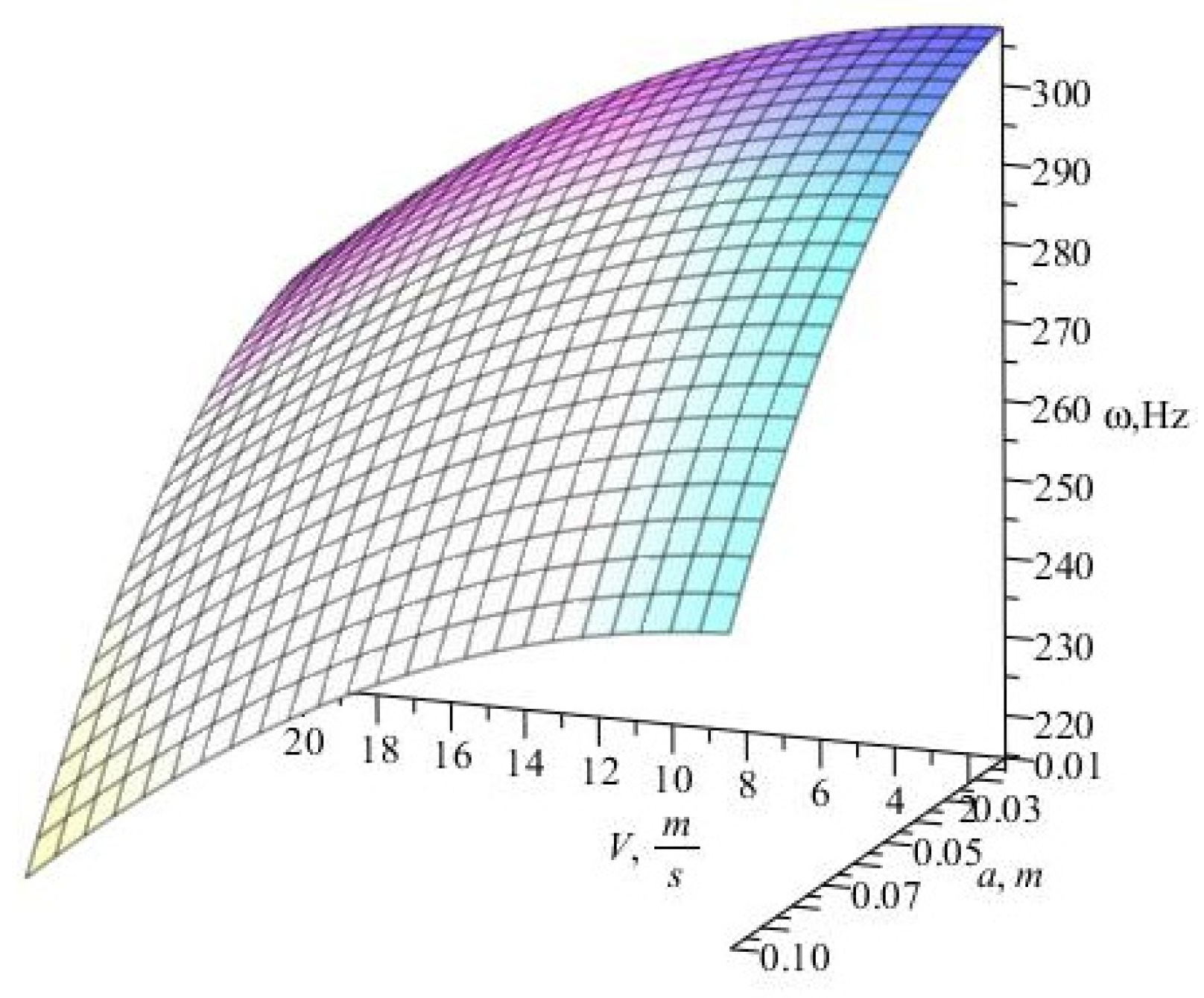
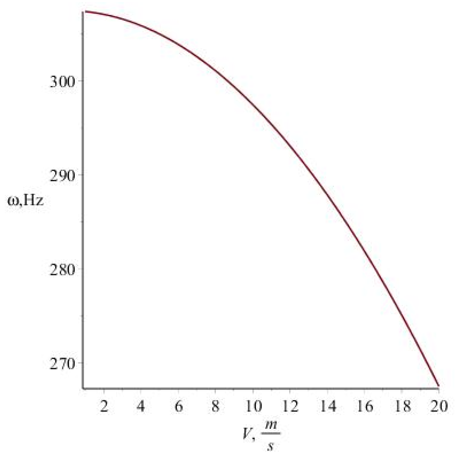
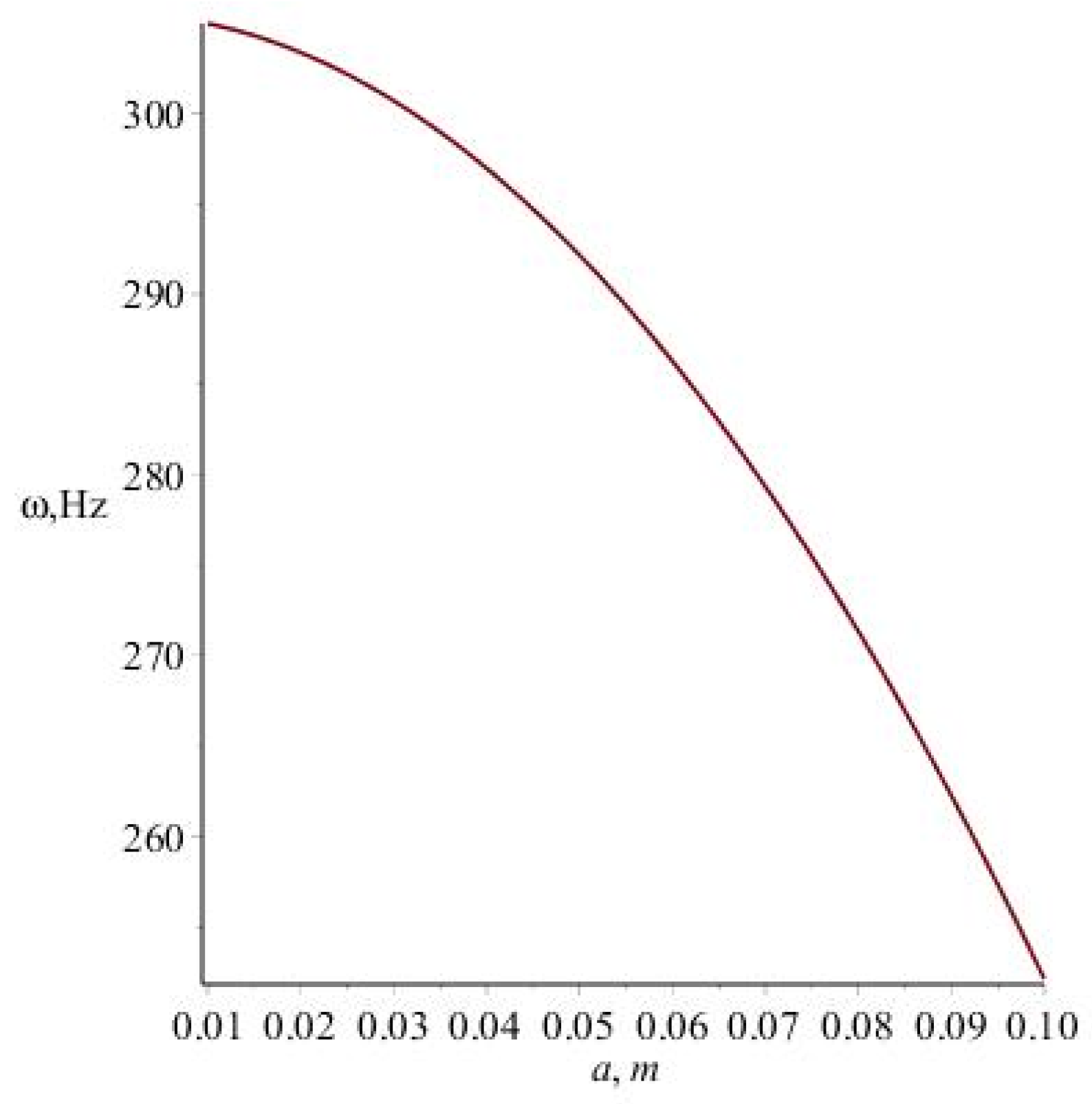
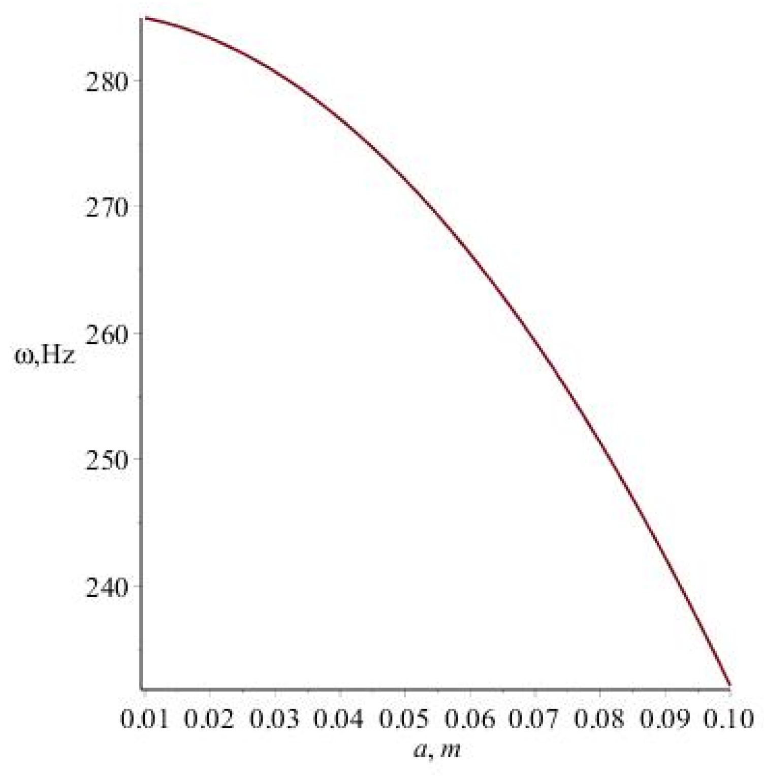
• After the graphical analysis of numerical simulations (Figure 2, Figure 3, Figure 4, Figure 5 and Figure 6) and the corresponding equation system, it can be concluded that the speed of movement reduces the frequency of vibrations (for the non-resonant case with hinged fastening), i.e., at $V=5 \mathrm{m}/\mathrm{s}$, the frequency of vibrations decreases almost to 2 Hz, and when the amplitude increases, the frequency decreases slightly (by 1%) according to the parabolic law, which is not as significant as when the longitudinal speed is affected.
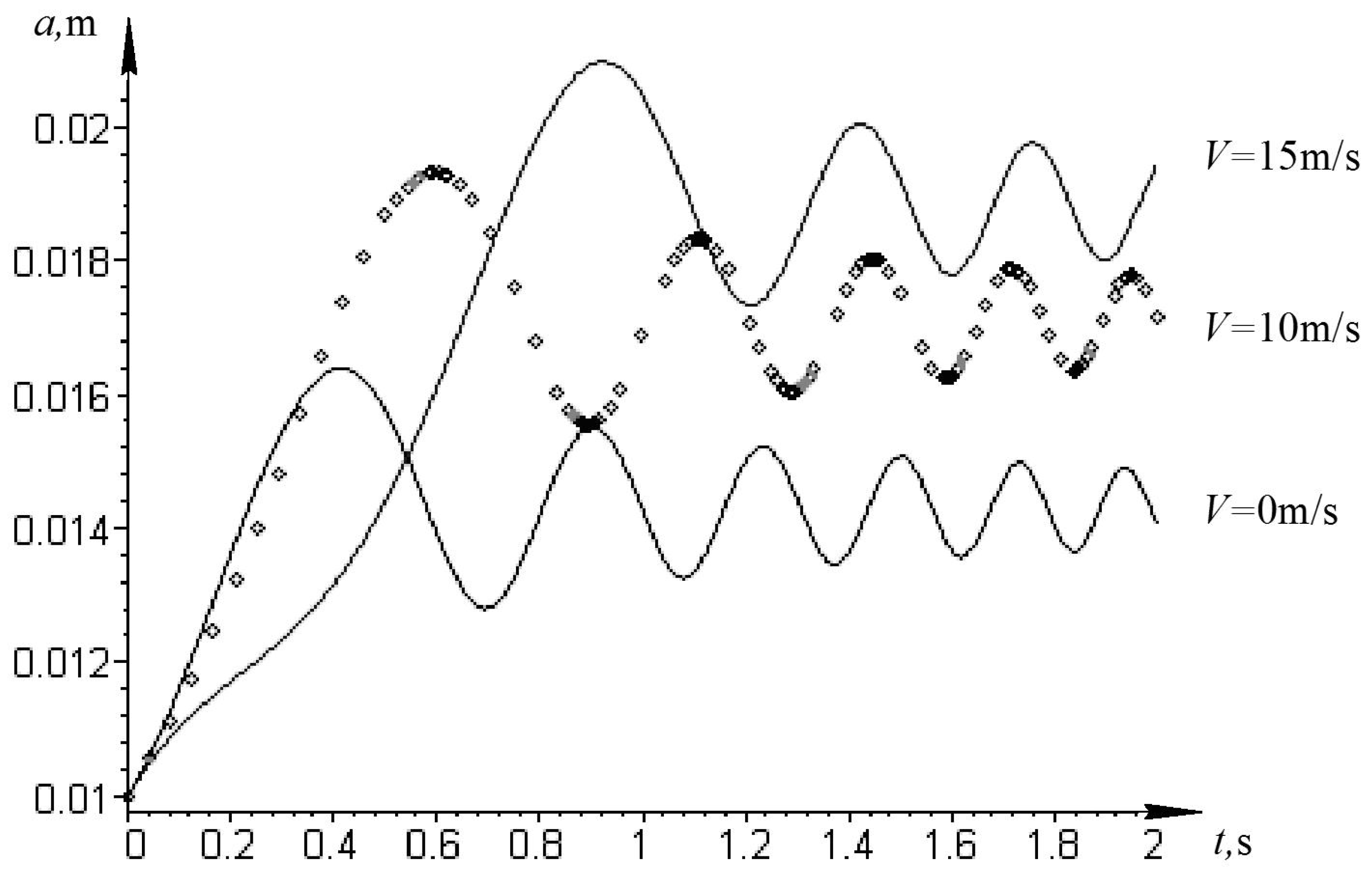
• Additionally, in the resonant case, it can be seen that an increase in the speed of medium movement leads to an increase in the amplitude. For example, at a speed of $V=15 \mathrm{m}/\mathrm{s}$, the amplitude of vibrations of the system increases by 22%. It can also be seen that the vibration frequency of the dynamic process decreases with increasing speed.
• The amplitude of vibrations of the system remains unchanged and is equal to its initial value, if the system is conservative ($a$ = const). The influence of speed on the change in system frequency is decreasing in nature; the higher the speed, the lower the system frequency.
• From the results of the work, as a special case, at $V\to 0$, we obtain results that are relative to quasi-linear systems with distributed parameters that are not characterized by longitudinal motion.
• The obtained mathematical models allow design engineers to take into account the influence of the characteristics listed in the study (speed, disturbing force, physical and mechanical characteristics of the beam material) even at the stage of designing homogeneous nonlinear elastic systems. The correlations obtained in the study make it possible to research the influence of the parameters of the moving medium on the nature of changes in the frequency and amplitude of vibrations and to predict dynamic phenomena in them with the required accuracy. If properly applied in engineering calculations of industrial equipment, the obtained dependences can be used for the synthesis and optimization of the parameters of pipelines, through which a liquid medium flows, and other similar structural elements.
• Practical applications of the obtained results in the paper are as follows:
  • Nonlinear transversal oscillations of the telescopic boom of a crane are studied as real phenomena. The numerical characteristics of the oscillating system considered in the paper relate to the mathematical model of the telescopic boom (CTD-KB P 3200 beam crane with two hooks). Optimization of parameters for such types of technological constructions can be predicted due to the considered procedure.
  • Substitution of some physical parameters in the proposed model enables us to consider mathematical models of nonlinear oscillations for liquid pipelines as well. Optimization of parameters can be realized in the same way also.

The authors’ plans for future study are to consider how the proposed procedure works in the case of more complicated forms of boundary value conditions.

References

1. Andronov, A.; Witt, A.A.; Khaikin, S.E. Theory of Oscillators; Addison-Wesley Publ. Company, Inc.: London, UK, 1966. [Google Scholar] [CrossRef]
2. Anisimov, I.O. Oscillations and Waves; Akadempress: Kyiv, Ukraine, 2003. [Google Scholar]
3. Zviaduri, V.; Chelidze, M.; Tedoshvili, M. Dynamics of Vibratory Technological Machines and Processes; Lambert Academic Publ.: Riga, Latvia, 2021. [Google Scholar]
4. Kneubühl, F.K. Oscillations and Waves; Springer: Berlin, Germany, 1997. [Google Scholar] [CrossRef]
5. Fidlin, A. Nonlinear Oscillations in Mechanical Engineering; Springer: Berlin, Germany, 2006. [Google Scholar] [CrossRef]
6. Wagg, D.; Neild, S. Nonlinear Vibration with Control; Springer Intern. Publ.: Basel, Switzerland, 2015. [Google Scholar] [CrossRef]
7. Andrukhiv, A.; Sokil, B.; Sokil, M. Resonant phenomena of elastic bodies that perform bending and torsion vibrations. Ukr. J. Mech. Eng. Mater. Sci. 2018, 4, 65–73. [Google Scholar] [CrossRef]
8. Pukach, P.; Slipchuk, A.; Beregova, H.; Pukach, Y.; Hlynskyi, Y. Asymptotic Approaches to Study the Mathematical Models of Nonlinear Oscillations of Movable 1D Bodies. In Proceedings of the 2020 IEEE 15th International Conference on Computer Sciences and Information Technologies (CSIT), Zbarazh, Ukraine, 23–26 September 2020; Volume 1, pp. 141–145. [Google Scholar]
9. Slipchuk, A.; Pukach, P.; Vovk, M.; Slyusarchuk, O. Advancing asymptotic approaches to studying the longitudinal and torsional oscillations of a moving beam. East.-Eur. J. Enterp. Technol. 2022, 3, 31–39. [Google Scholar] [CrossRef]
10. Yurish, S.Y. Sensors and Biosensors, MEMS Technologies and Its Applications. In Advances in Sensors: Reviews; International Frequency Sensor Association Publ.: Barcelona, Spain, 2014; Volume 2. [Google Scholar]
11. Sokil, B.I.; Khytriak, O.I. Vibrations of drive systems flexible elements and methods of determining their optimal nonlinear characteristics based on the laws of motion. Mil. Tech. Collect. 2009, 2, 9–12. [Google Scholar] [CrossRef]
12. Mittal, P.K. Oscillations, Waves and Acoustics; I.K. International Publishing House Pvt. Ltd.: New Delhi, India, 2010. [Google Scholar]
13. Firouz-Abadi, R.D.; Haddadpour, H.; Novinzadeh, A.B. An asymptotic solution to transverse free vibrations of variable-section beams. J. Sound Vib. 2007, 304, 530–540. [Google Scholar] [CrossRef]
14. Wang, Y.; Zhu, W. Supercritical nonlinear transverse vibration of a hyperelastic beam under harmonic axial loading. Commun. Nonlinear Sci. Numer. Simul. 2022, 112, 106536. [Google Scholar] [CrossRef]
15. Sah, S.M.; Thomsen, J.J.; Tcherniak, D. Transverse vibrations induced by longitudinal excitation in beams with geometrical and loading imperfections. J. Sound Vib. 2019, 444, 152–160. [Google Scholar] [CrossRef]
16. Gritsenko, D.; Xu, J.; Paoli, R. Transverse vibrations of cantilever beams: Analytical solutions with general steady-state forcing. Appl. Eng. Sci. 2020, 3, 100017. [Google Scholar] [CrossRef]
17. Cao, D.; Gao, Y.; Wang, J.; Yao, M.; Zhang, W. Analytical analysis of free vibration of non-uniform and non-homogenous beams: Asymptotic perturbation approach. Appl. Math. Model. 2018, 65, 526–534. [Google Scholar] [CrossRef]
18. Lenci, S.; Rega, G. An asymptotic model for the free vibrations of a two-layer beam. Eur. J. Mech.-A/Solids 2013, 42, 441–453. [Google Scholar] [CrossRef]
19. Ahmed, A.; Rhali, B. Geometrically nonlinear transverse vibrations of Bernoulli-Euler beams carrying a finite number of masses and taking into account their rotatory inertia. Procedia Eng. 2017, 199, 489–494. [Google Scholar] [CrossRef]
20. Torabi, K.; Jazi, A.J.; Zafari, E. Exact closed form solution for the analysis of the transverse vibration modes of a Timoshenko beam with multiple concentrated masses. Appl. Math. Comput. 2014, 238, 342–357. [Google Scholar] [CrossRef]
21. Serpilli, M.; Lenci, S. Asymptotic modelling of the linear dynamics of laminated beams. Int. J. Solids Struct. 2012, 49, 1147–1157. [Google Scholar] [CrossRef] [Green Version]
22. Won, H.-I.; Chung, J. Numerical analysis for the stick-slip vibration of a transversely moving beam in contact with a frictional wall. J. Sound Vib. 2018, 419, 42–62. [Google Scholar] [CrossRef]
23. Babaei, M.; Asemi, K.; Safarpour, P. Natural frequency and dynamic analyses of functionally graded saturated porous beam resting on viscoelastic foundation based on higher order beam theory. J. Solid Mech. 2019, 11, 615–634. [Google Scholar] [CrossRef]
24. Lv, H.; Li, Y.; Li, L.; Liu, Q. Transverse vibration of viscoelastic sandwich beam with time-dependent axial tension and axially varying moving velocity. Appl. Math. Model. 2014, 38, 2558–2585. [Google Scholar] [CrossRef]
25. Qaderi, S.; Ebrahimi, F.; Vinyas, M. Dynamic analysis of multi-layered composite beams reinforced with graphene platelets resting on two-parameter viscoelastic foundation. Eur. Phys. J. Plus 2019, 134, 1–11. [Google Scholar] [CrossRef]
26. Vîlcu, R.; Bala, D. Particularities of some proposed models for the characterization of chemical oscillations. Model. Oscil. Chem. React. 2004, 277–286. [Google Scholar]
27. Shesha Prakash, M.N.; Suresh, G.S. Textbook of Mechanics of Materials; PHI Learning Private Limited: New Delhi, India, 2011. [Google Scholar]
28. Bogolyubov, N.N.; Mitropolsky, Yu.A. Asymptotic Methods in the Theory of Non-Linear Oscillations; Hindustan Publ. Corp.: New Delhi, India, 1961. [Google Scholar]
29. Tsmots, I.; Rabyk, V.; Kryvinska, N.; Yatsymirskyy, M.; Teslyuk, V. Design of the Processors for Fast Cosine and Sine Fourier Transforms. Circuits Syst. Signal Process. 2022, 1–24. [Google Scholar] [CrossRef]
30. Davis, H.F. Fourier Series and Orthogonal Functions; Dover Publications, Inc.: New York, NY, USA, 2012. [Google Scholar]
31. Fetter, A.L.; Walecka, J.D. Nonlinear Mechanics; Dover Publications, Inc.: New York, NY, USA, 2006. [Google Scholar]
32. Sharma, A.K. Textbook of Differential Equations; Discovery Publishing House: New Delhi, India, 2010. [Google Scholar]
33. Dronyuk, I.; Fedevych, O.; Kryvinska, N. Constructing of Digital Watermark Based on Generalized Fourier Transform. Electronics 2020, 9, 1108. [Google Scholar] [CrossRef]
Figure 1. Schematic model of a beam moving along its axis.
Mathematics 11 00322 g001