1. Introduction
A sales funnel is a marketing model that describes the expected “journey” of a future customer from first encountering an offer or product to real purchase. The research by Venermo, A., Rantala, J., and Holopainen, T. states that the stages of a client’s “journey” are points of contact with the client, which are cases when the client contacts the company and its brand [
1]. Any modern business has an urgent need to track the stages of transactions and the effectiveness of the sales and marketing departments. A sales funnelallows the whole sales process to be divided into a number of stages [
2]. Different companies interpret the stages of deals in sales funnels differently, but every sales funnel always has two main stages: opening and closing a deal.
Analyzing the sales funnel is a time-consuming task. As a rule, analysis comes down to finding emerging constraints and is directly related to E. Goldratt’s theory of constraints [
3]. Analysis helps to quickly find the bottlenecks in the funnel and understand where employees and the company make the most mistakes, starting from attracting the customer and ending with further support of the sold product. The goal of the analysis is to find bottlenecks in the funnel and understand where customers stop, and for what reason they do so. Ideally, every stage of the sales funnel should be digitized and its accounting should be automated.
The most viable sales funnel consists of at least four stages in which the customer asks questions about the importance of the company’s offer to him or her each time. The research by Vasilieva, E., and Loseva, V., says that the process of customer movement consists of a number of steps that can be graphically represented as an inverted pyramid, with a wide edge at the top, where the interest of a potential customer is represented, and a narrow neck at the bottom, where the number of purchases of the proposed product is shown. The customer is passed through the sales funnel from familiarization with the product to its purchase, answering the following questions himself [
4]:
Do I know and understand the company’s offer?
Do I like the product and price offered?
Am I able and willing to buy the company’s product?
How do I buy the product I’ve learned about?
At all stages of the sales funnel, a company is capable of making many mistakes. Sales funnel analysis helps to see these mistakes and take action to correct them. The company should use all the data available to it, as well as introduce additional metrics. All available data should be obtained without much effort and unnecessary cost, as it should not increase the cost of maintaining the sales funnel. The study by Krause, O., and Pinyak, I., states that marketing analysis of the sales funnel should be carried out in order to maximize the efficient use of the company’s resources, as well as for optimal structuring of existing marketing and sales processes. Thus, it is necessary to select the most needed data set, without artificially expanding it [
5]. Conducting sales funnel analysis allows a company’s management to not rely on intuition, but to see the actual data as it is. Conducting an analysis significantly increases the speed of finding problems and ways to solve them.
The sales funnel has its own unique appearance in each company and industry. The structure of the funnel also depends on the marketing strategy of the company and the activities of the sales department. Each funnel is divided into two large stages. In the first stage of the sales funnel, the marketing departments always do the bulk of the work and in the second stage, the sales departments do the bulk of the work. The marketing department must determine the company’s target audience, find the channels in which customers are most often interested in the product, and convey the company’s offer to the customer. In turn, the sales department should bring the potential client to the purchase, as well as provide support in the use of a product or service. All sales funnels can be divided into two quite conventional types—basic and advanced. The basic sales funnel consists of four stages: attention, interest, desire, and action. The extended sales funnel can modify these stages and add new ones, such as support and repeat purchase, etc.
We shall take a closer look at the most popular methods of sales funnel analysis [
6,
7]. The methods for analyzing the stages of the sales funnel largely depend on the industry in which the sales funnel is used. It is accepted to distinguish three main big groups of methods for sales funnel analysis.
The first group of methods are “informative” methods. The methods in this group focus on testing changes in the stages of the sales funnel. This group of methods includes A/B testing, comparative analysis of competitors’ advertising campaigns, and measurement of a company’s brand awarenessю. The study by Szymkowiak, A., says that such methods allow for analysis without using any additional tools, such methods allow for a superficial analysis of sales funnels [
8].
The second group of methods are methods of comparison with competitors. These methods are mostly aimed at changing the sales funnel based on the activities of competitors. They take into account both positive and negative experiences of competitors’ sales funnels. The purpose of this group is to determine what a customer finds value in from a competitor’s product. The analysis can include a variety of parameters of the product being sold that can be compared to the competitor’s products. Additionally analyzed can be the support services of the company conducting the analysis and the competitors’ support services, the different sales channels and their effectiveness, and the methods of salespeople, etc. The research by Bogetić, Z., Stojković, D. and Dokić, A., states that methods of comparison with competitors are a vital necessity since without these methods, it is impossible to correctly assess competition in the market, which leads to financial losses [
9].
The third group of methods is directed to the “making of purchase”. This group of methods considers the process of attracting the customer to buy a product and are aimed at testing the marketing strategies of the company. This group includes a method of experiment and a method of comparative evaluation of competitors’ sales services activity. These methods allow answering of the questions including whether the product is positioned correctly in the market, why the customer buys it, and how much they are ready to pay for the product. The research conducted by Miletić, V., Grubor, A., and Čurčić, N., says that the correct positioning of the goods on the market is the main necessity since a potential customer must find the company’s goods in the easiest way. Each additional step that the customer will take in the search for a product carries a decrease in the probability of purchase [
10].
Sales funnel analysis is a vital necessity for most companies, because if it cannot be understand as to how a customer comes to buy a product, one cannot scale the business and develop new products. Sales funnel analysis allows the identification of significant errors at many different stages of the sales funnel. Sales funnel analysis allows the company management to look at the marketing and sales process from the outside and decide how to improve it. The methods described earlier can be combined with each other, but company management should keep in mind that certain methods may not be suitable for the chosen product niche or industry at all.
Another task of working with sales funnels is forecasting future sales. This is quite a time-consuming task, and the resulting forecasts are mainly based on the identification of hidden patterns in the accumulated data [
11]. Sales funnel forecasting helps to save the advertising budget and plan the future promotion and sales strategy of the company. The exact forecast can help to reveal shortcomings in methodologies of marketing and sales departments; in ineffective sales channels; in predictions of seasonal growth and declines in sales, etc. The earlier a company starts forecasting its sales funnels, the more time it will have to solve problems.
Using the past to predict the future is the basis of forecasting sales funnels. At the same time, the accumulated data can be used in different ways. You can choose among the following groups of methods:
Expert forecasting. Qualitative methods of sales forecasting models are used when there is a limited amount of data available. In this group of methods, forecasting relies on human judgment and gut feeling, and the task is to turn the resulting estimates into a final quantitative forecast. The purpose of the method is to combine all judgments and information about the evaluated factors in a logical and systematic way [
12].
Analytical forecasting. Time series analysis methods for sales forecasting are used when there is a large amount of data for different periods about a product or product line. They can be used when there are clear product sales trends, and they are stable. The forecaster uses past product sales data to get the projected sales value and the change in sales rate at this time and for future periods [
13].
Causal methods. Causal forecasting models are developed when sufficient historical product data is available. The analysis should show the factors to be predicted and other economic forces and socio-economic factors. If complex sales forecasting models are needed, a causal model should be used. It expresses an appropriate causal relationship and can include market survey information and other considerations. The method can also include the results of time series analysis. This group of methods is quite expensive and very time-consuming to develop and maintain [
14,
15].
2. Choice of Method for Forecasting Sales Funnels
2.1. Overview of Methods for Forecasting Sales Funnels
Sales forecasting helps you properly allocate the costs of your sales funnel, as well as build your advertising strategies. It was described earlier that there are three most popular groups of sales forecasting methods. Within these groups, there are a huge number of methods. It is necessary to choose the most universal and simple method for further use in forecasting by inexperienced users. We shall consider each group of methods one by one [
16].
Expert forecasting is used with a limited amount of data, but it strongly depends on the human factor in the form of estimations and opinions of experts [
17]. With a high degree of confidence, we can say that forecasts using methods from this group will always be considerably different from the real values, but for the sake of the purity of the experiment, one method from this group will be compared to methods from other groups. From this group, it was decided to consider the method “sales staff opinion” [
18].
The methods that make up a fairly extensive group of methods “Analytical forecasting” are mainly time series analysis methods. This group of methods can be used when a company has an accumulated amount of data for different periods (each method has its own recommendations for the number of periods). Furthermore, these methods are suitable for looking at a single product rather than an entire product line. The forecaster can use historical sales funnel data to get a projected sales value and predict sales trends from period to period. To further select the best method for forecasting sales funnels, three of the most popular methods in this group were selected. The selected methods were past sales turnover, forecast with growth and seasonal coefficients, and forecast by Holt’s exponential smoothing method. Instead of Holt’s exponential smoothing method, other methods of time series analysis can be used, but they will not give significant changes in the results of forecasting. The Holt exponential smoothing method was chosen because it is easy to implement and lends itself well to modifications [
19,
20,
21].
Although methods belonging to the “causal” group are considered the most accurate in the field of forecasting, they will not be considered in the comparison because they require more data than can be accounted for by a sales funnel. Working with these methods also requires extensive knowledge of mathematics, which may discourage many companies from forecasting sales funnels [
14,
15].
2.2. Comparison of Sales Funnel Forecasting Methods
The selected methods will be compared by the following criteria: relative forecasting error, the required number of time periods, requirements to the quality of initial data, and complexity of implementation within a universal method for most companies. The initial data quality requirement is understood as the presence of significant deviations in the periods, which can affect the forecasting method.
Test data will be used as real sales data of the product “Tooth harrow (200 mm)” of the company, which produces spare parts and agricultural machinery. This is a fairly inexpensive and quickly consumable spare part for a heavy harrow manufactured by the company. The part is also suitable for heavy harrows from other manufacturers, so the company has several different sales channels. The number of products sold increases every year.
Table 1 shows the sales of “Tooth harrow (200 mm)” for different years. Based on this data, we shall compare the previously selected methods. This amount of data is sufficient for forecasting by the methods under consideration. For some methods, additional data will be used, which will be refined as the experiments are described.
2.3. Forecasting by the Method of “Sales Staff Opinion”
First, we shall consider the “sales force opinion” method. Each of the employees of the sales department gives three forecasts: the minimum achievable, the most realistic, and the maximum achievable (taking into account production limitations). The evaluation conducted by sales employees also includes the evaluation for the five main sales channels [
22]. On the basis of their forecasts using Equation (1), the final forecast is calculated:
where
Cj—forecast sales volume;
min—minimum sales forecast according to the employee;
real—realistic sales forecast according to the employee;
max—maximum sales forecast according to the employee.
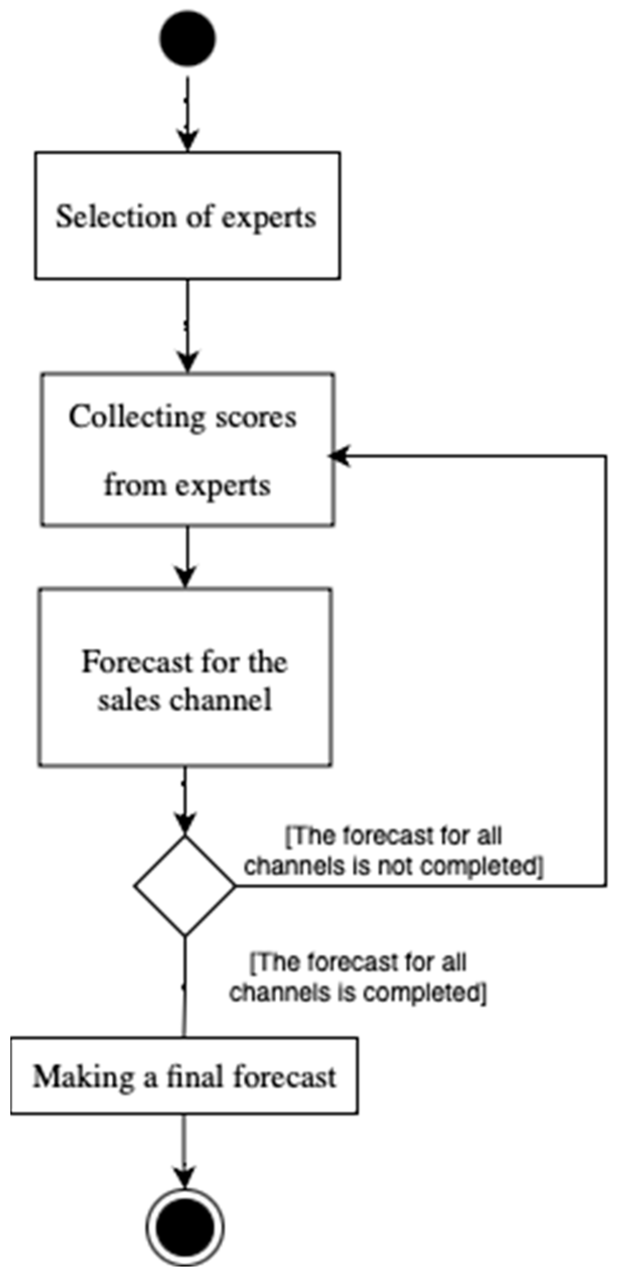
If we present the algorithm of the method in steps, then it will take the following form:
Step 1. Selection of experts. At this step, it is necessary to select experts who will participate in forecasting;
Step 2. Collecting scores from experts. It is necessary to get the minimum, realistic, and maximum forecast for the sales channel from the sales department employee who manages the sales channel;
Step 3. Forecast for the sales channel. At this step, sales are predicted using Equation (1);
Step 4. Check that the forecast is received for all sales channels. If the forecast is received for each sales channel, then you can proceed to Step 5. If the forecast is not received for all sales channels, then you need to go back to Step 2 and make a forecast for a new sales channel;
Step 5. Making a final forecast. At this step, it is necessary to sum all the forecasts obtained using Equation (1) to obtain the final total forecast.
The algorithm of forecasting by the method “sales staff opinion” is also presented on the UML activity diagram in
Figure 1.
The company previously used the sales staff’s opinion to forecast sales and production, so the company was able to get the results of forecasting for 2021. The results of forecasting are presented in
Table 2.
The total forecast was 64,579 units of the product. According to the results of 2021, it was actually possible to sell 55,028 units of the product. Thus, the accuracy of the forecast was 82%. This is quite a low accuracy and all of the three types of forecasts (minimum, maximum, and realistic) also have low accuracy.
For expert forecasting, it does not make sense to make a forecast for a longer period, since a significant proportion of the human factor is present in this method. The company’s employees can estimate the demand for the coming year based on past data but, for example, for the second year of forecasting, they cannot rely on existing data. Employees of the sales department, for the second and subsequent years, cannot take into account the possibility of a drop in demand for a product or, conversely, its explosive growth. Even if they make several forecasts for different scenarios, the management of the company will not be able to choose a specific scenario.
2.4. Forecasting by the “Past Sales Turnover” Method
We shall move on to analytical forecasting methods. To begin with, let us carry out forecasting by the method of “past sales turnover” [
23]. This method will be used to make forecasts for the year 2021. The first step of this method is to make a forecast for 2020 using 2018 and 2019 data by the following Equation (2):
where
X is next year’s turnover,
A is this year’s turnover, and
B is last year’s turnover.
The forecast for 2020 was 59,948 units of production. Actual sales for 2020 were 52,985 units. The accuracy of the forecast in the first iteration was 86.8%. This is also a rather low accuracy but is not the end of forecasting with this method.
The second step is to calculate sales forecast for 2021 on the basis of 2019 and 2020 data using Equation (2) and make a correction for accuracy calculated in the first step. It should be emphasized that the correction for accuracy makes sense only if sales fluctuate by more than 10% compared to the previous year, otherwise the correction is not necessary.
The forecast for 2021 was 62,818 units. The actual increase in sales in 2020 to 2019 was approximately 19%. According to this method, with this increase in sales (more than 10%), an adjustment for accuracy on the 2020 forecast result is necessary for the forecast. That is, the 2021 forecast must be multiplied by the accuracy of the 2020 forecast.
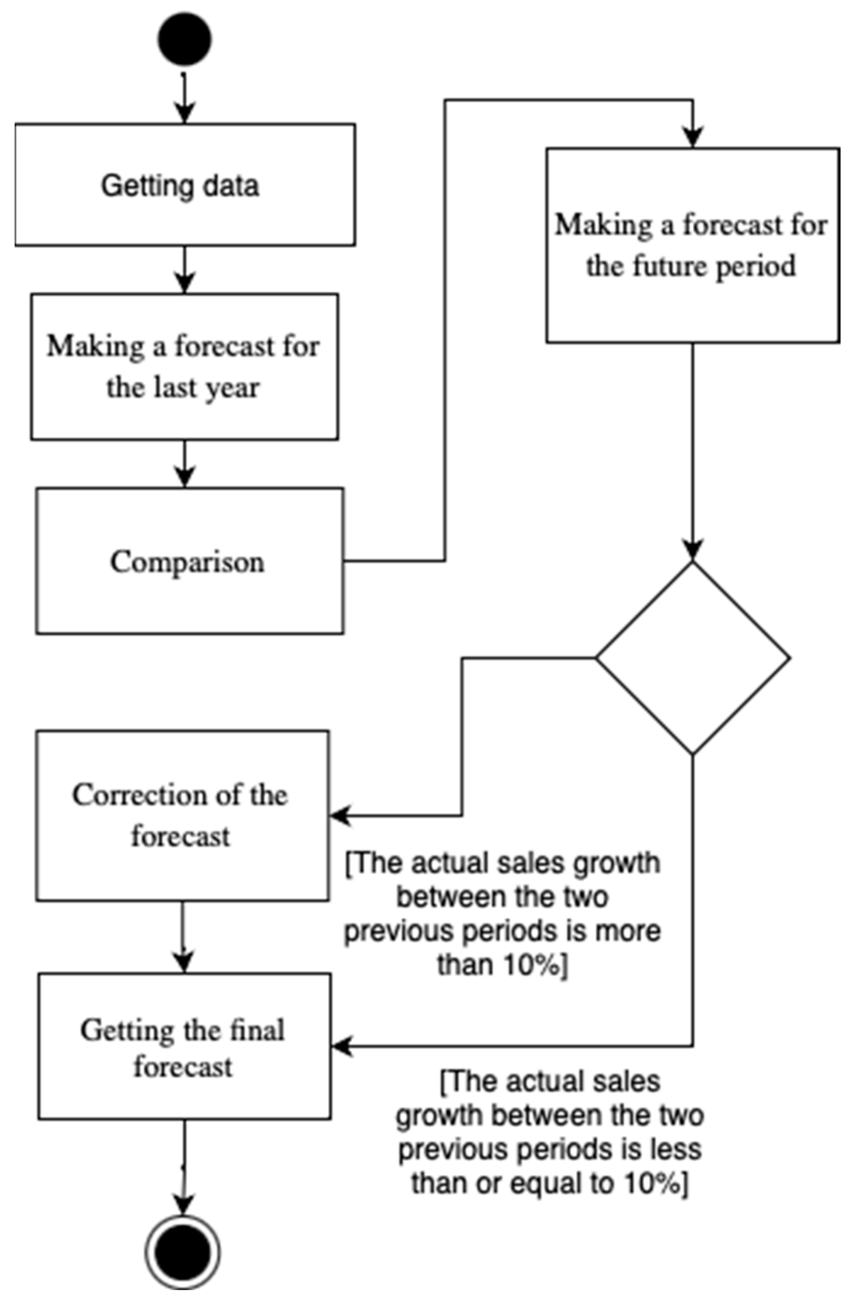
If we present the algorithm of the method in steps, then it will take the following form:
Step 1. Getting data. At this step, you need to get sales data for previous periods (when forecasting for 1 year, you need to get data for 2 previous years);
Step 2. Making a forecast for the last year. It is necessary to make a forecast for the last known year before the start of forecasting future periods. This calculation can be performed according to Equation (2);
Step 3. Comparison. This step compares the increase in sales between the last two known periods. If the increase is more than 10%, then will need to use Step 5, if the increase is less than 10%, then the prediction is completed at Step 4;
Step 4. Making a forecast for the future period. Such a calculation can be performed according to Equation (2). If the increase in sales between the two previous periods is less than 10%, then the resulting forecast does not need to be finalized;
Step 5. Correction of the forecast. The forecast is adjusted by multiplying the received forecast for the future period by the accuracy of the forecast made in Step 2.
The final algorithm for forecasting by the “past sales turnover” method is presented in the UML activity diagram in
Figure 2.
The final forecast, adjusted for accuracy, was 55,531 units. The actual order volume for 2021 was 55,028 units. The accuracy of the forecast adjusted for accuracy of the previous year was 99.1%.
The “past sales turnover” method uses several periods at once to achieve an accurate forecast. To begin with, in this method, it is necessary to make a forecast for one period and compare it with real results. Only then can we move on to forecasting the future period. Since we do not know the final sales data of the forecast period, we cannot calculate the correction for accuracy and therefore we cannot forecast for additional periods, since we cannot guarantee the adequacy of the forecasts received.
2.5. Forecast with Growth and Seasonal Coefficients
The process of forecasting with growth and seasonality coefficients relies on data on previous sales for a minimum of 36 periods, ideally 60 periods or more. This required number of periods already creates certain difficulties, if there are not enough data for forecasting. The process of forecasting by this method is conditionally divided into three stages. First, it is necessary to calculate the trend value used for forecasting. The next stage is the determination of seasonality coefficients. At the end, it is necessary to carry out sales forecasting [
24].
To begin with, it is necessary to calculate the linear trend coefficients y = bx + a, using the method of least squares.
Table 3 presents the results of the calculations.
Next, we calculate the values of the trend. To do this, the values of trend coefficients should be inserted into the previously used formula y = bx + a. Instead of “x” we should substitute the number of periods in time series from 1 to 36. Thus, we can get “y” values of linear trend for each period.
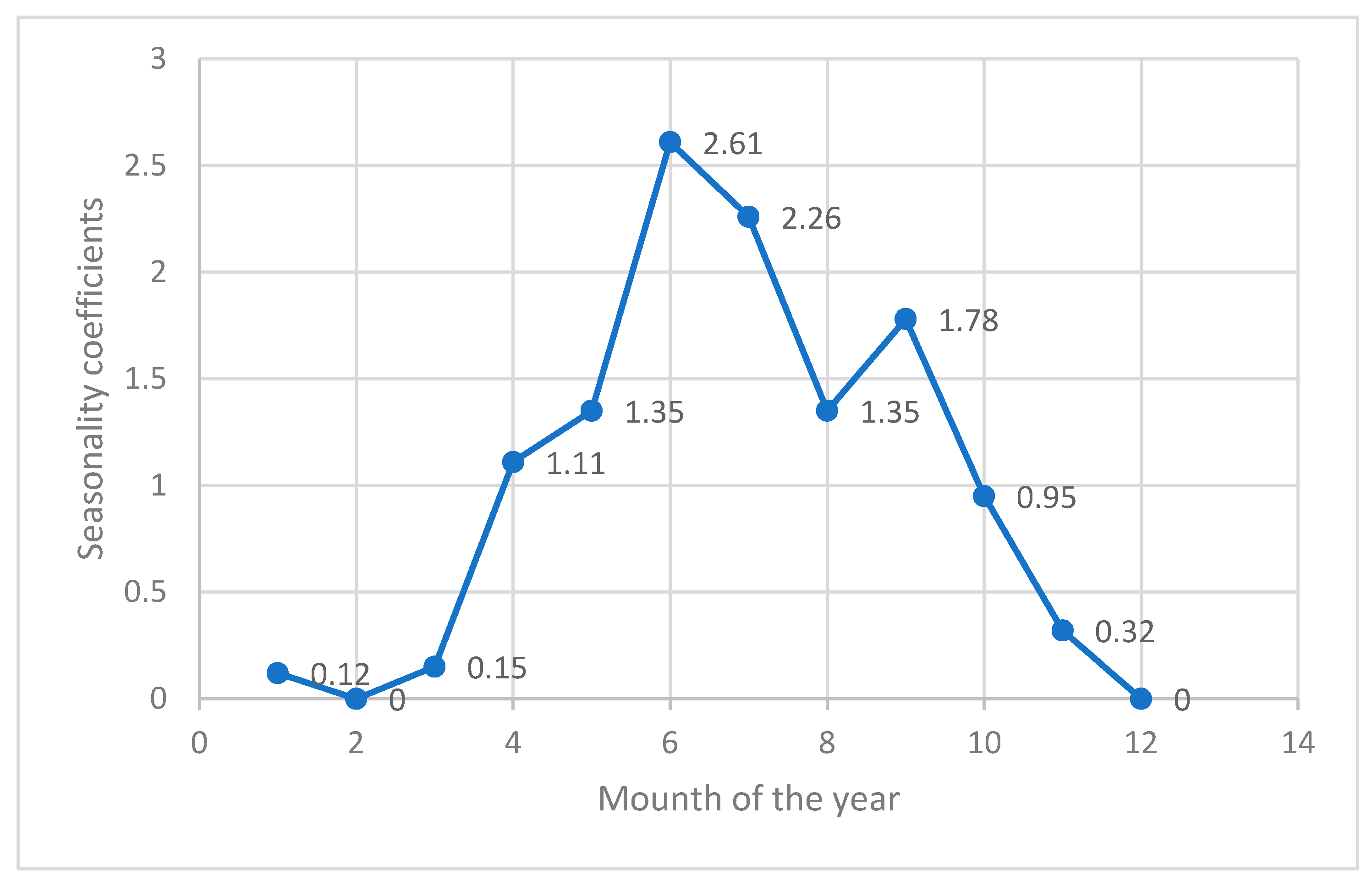
The next step is to determine the coefficients of seasonality. It is necessary to calculate the deviation of actual values from the trend values. For this purpose, the actual values should be divided by the trend values. For each period the average deviation for 36 months and the total index of seasonality is found. The seasonality coefficients are calculated by dividing each value of the average deviation by the total seasonality index. An example of calculations for 12 periods is presented in
Table 4.
Figure 3 shows the curve of seasonality coefficients, cleared from growth.
As can be seen from
Figure 3, the coefficient of seasonality increases from the spring period and falls at the end of autumn. Such different values of the coefficients are due to the fact that the products produced by the company are more often purchased during the sowing period in the fields, as well as during the processing and harvesting periods. The company’s products are represented only in one country, in which there are practically no agricultural works in winter.
The last step is forecasting. To do this, it is necessary to set the period for which the forecast is needed. The period is set by extending the time series by 1 year (12 periods) or any greater value. Trend value is also calculated for future periods (by substituting new periods into “x” value of the equation y = bx + a). In order to make forecasts, it is necessary to multiply linear trend values by seasonal coefficients. The results of the calculations are presented in
Table 5.
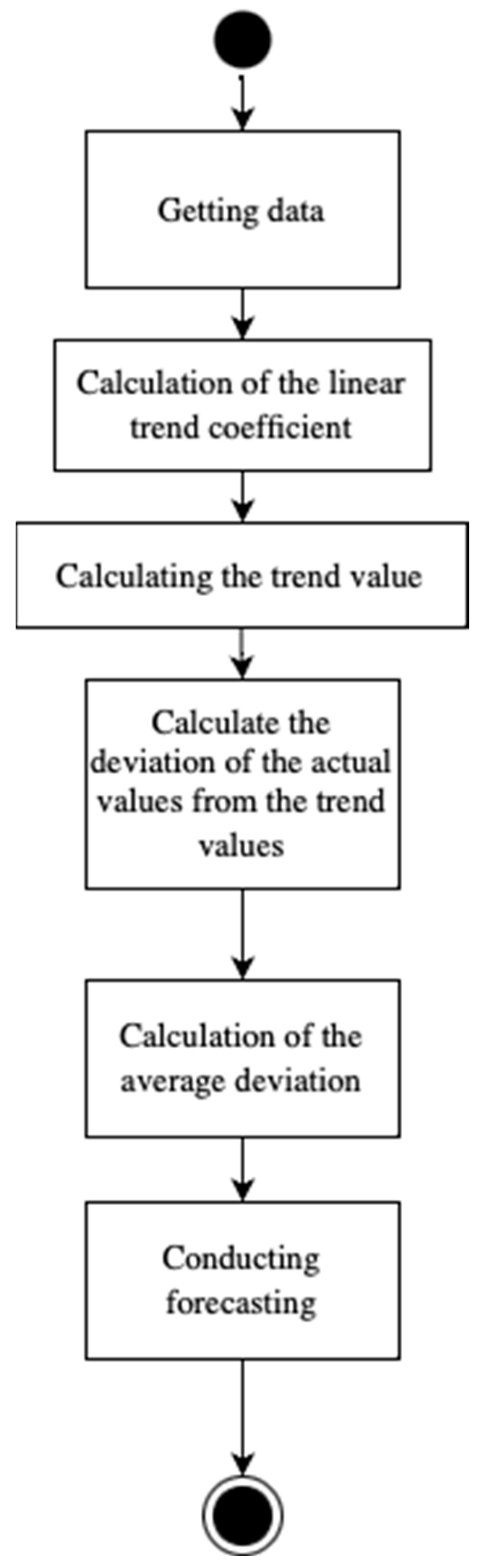
If we present the algorithm of the method in steps, then it will take the following form:
Step 1. Getting data. At this step, you need to get sales data for previous periods (when forecasting for 1 year, you need from 36 to 60 periods (months));
Step 2. Calculation of the linear trend coefficient. This calculation can be performed according to Equation (3);
Step 3. Calculating the trend value. To do this, it is necessary to substitute the values of the trend coefficients in the previously used formula y = bx + a. Instead of “x”, we substitute the number of periods in the time series from 1 to 36, 48 or 60;
Step 4. Calculate the deviation of the actual values from the trend values. To do this, it is necessary to divide the actual values into trend values;
Step 5. Calculation of the average deviation. For each period, the average deviation for 36 months and the overall seasonality index are found. The seasonality coefficients are calculated by dividing each value of the average deviation by the total seasonality index;
Step 6. Conducting forecasting. To do this, we need to set the period for which the forecast is required. The period is set by lengthening the time series by 1 year (12 periods) or by any larger value. The trend value for future periods is also calculated (by substituting new periods into the value “x” of the equation y = bx + a). To make forecasts, it is necessary to multiply the values of the linear trend by seasonal coefficients.
The final algorithm when forecasting with growth and seasonality coefficients is presented in the UML activity diagram in
Figure 4.
The forecast for 2021 using this method was 67,405 units of production. The actual volume of products sold in 2021 was more modest 55,028 units of production. Thus, the final accuracy of the forecast was 77.5%. The final result is influenced by the emissions in some months, but this method does not provide the ability to smooth them. Such prediction accuracy is very low and in the future, when working with this method, it may lead to significant errors.
The considered method can carry out forecasting for additional periods, but when forecasting additional periods, it is necessary to use the data of the first forecast periods. As noted earlier, in this method, the forecast is affected by outliers, smoothing of which is not provided. Since the main forecast was obtained with emissions from earlier periods, all forecasts for additional periods will also be affected by emissions from previous periods and additionally by emissions from the first forecast period. Thus, making a forecast for additional periods using this method does not make sense.
2.6. Forecasting by “Holt Exponential Smoothing” Method
The last forecasting method that will be considered is Holt’s exponential smoothing method. It is quite similar in steps to the previous method, but differs in the formulas needed for calculation.
The key difference between Holt’s exponential smoothing method and the previous method is a lower requirement for the number of periods (to forecast for 1 year 12 periods are enough, for 6 months 6 periods are enough, etc.) [
25]. Also, this method is suitable if the data for previous periods have a tendency to a sharp change in values. This method can be modified to improve the values.
The first step is the calculation of exponentially smoothed series. This is a popular method for predicting time series (Equation (3)):
where
Lt is the smoothed value referring to the current period;
Lt−1 is the smoothed value referring to the previous period;
Tt−1 is the trend value referring to the previous period;
k is the series smoothing coefficient; and
Yt is the current value of the series.
Next, it is necessary to draw a trend line and determine all trend values (Equation (4)):
where
Tt—trend value relating to the current period;
Lt—exponentially smoothed value relating to the current period;
Tt−1—trend value relating to the previous period;
b—trend smoothing coefficient; and
Lt−1—exponentially smoothed value relating to the previous period.
The last step is the Holt exponential smoothing forecast for each predicted parameter (Equation (5)):
where
Ŷt+p is the Holt forecast referring to the “
p” period;
p is the ordinal number of the period for which the forecast is made;
Tt is the trend value referring to the last period; and
Lt is the exponentially smoothed value referring to the last period.
The principle of solution by this method is almost the same as the previous method, so you can immediately consider the prediction results, which are shown in
Table 6.
The final predicted value was 51,784 parts and the prediction accuracy was 94%. At first glance, the accuracy seems high enough, but another important property of Holt’s exponential smoothing method is that it is possible to track outliers and make necessary modifications. By modifying Holt’s exponential smoothing method, the accuracy can be increased. As we can see from the obtained values, the forecast values of September and December look very strange as they are outliers. It is necessary to detect outliers of the following nature: additive, level shift, seasonal additive, and local trend. By reducing the outliers, the forecast has changed significantly. We also modified this method by adding an unexpected growth coefficient to it. Such a coefficient is responsible for the assumed parameter that the company’s managers, when making forecasts, may assume that the product will fall into a buying trend next season or vice conversely may become outdated and lose its market positions. To add this method, the original Equation (5) was modified and presented in Equation (6):
where
Ŷt+p is the Holt forecast referring to the “
p” period;
p is the ordinal number of the period for which the forecast is made;
Tt is the trend value referring to the last period;
Lt is the exponentially smoothed value referring to the last period; and
Ct is the coefficient of unexpected growth.
Table 7 shows the results of the forecast with smoothed outliers.
Table 8 shows the results of the forecast with smoothed emissions and an additional variable
Ct, which is 1.25 (assuming that sales will be 25% higher).
Table 9 shows the results of the forecast with smoothed emissions and an additional variable
Ct, which is 0.8 (assuming that sales will be 20% lower).
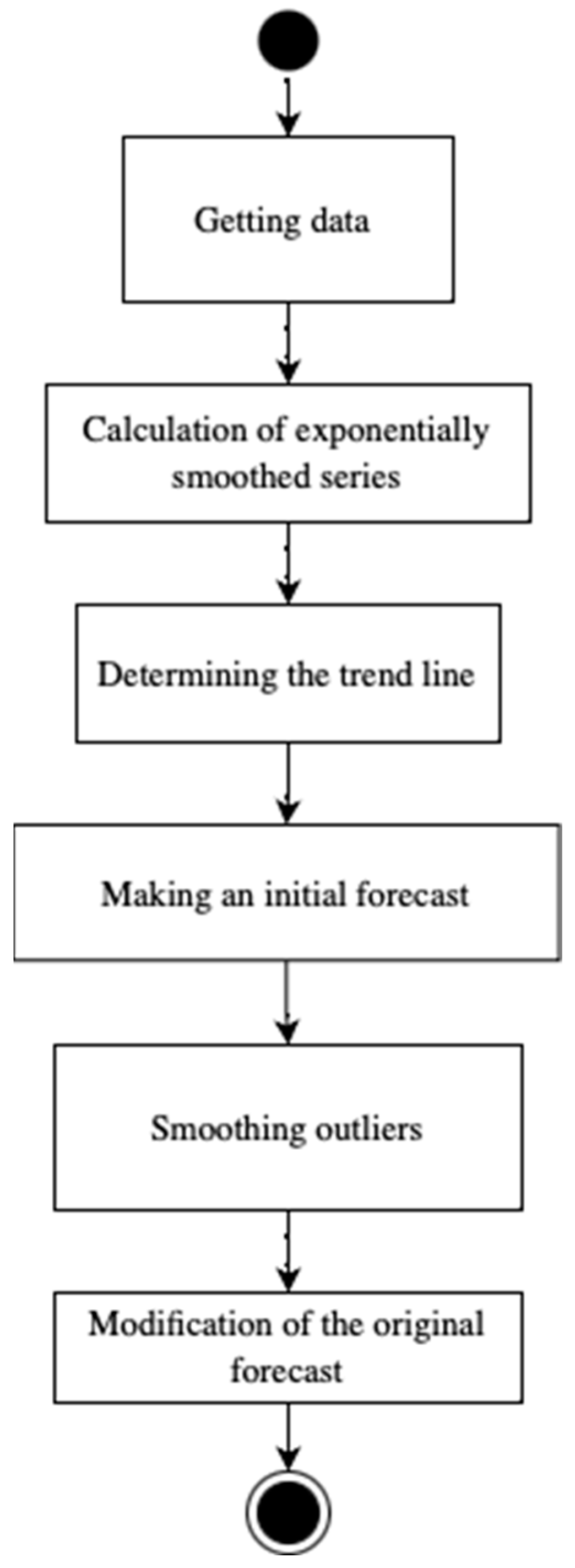
If we present the algorithm of the method in steps, then it will take the following form:
Step 1. Getting data. At this step, we need to get sales data for previous periods (when forecasting for 1 year, this is 12 periods);
Step 2. Calculation of exponentially smoothed series. This calculation can be performed according to Equation (3);
Step 3. Determining the trend line. It is necessary to draw a trend line and determine all trend values using Equation (4);
Step 4. Making an initial forecast. Making a forecast using the Holt exponential smoothing method using Equation (5);
Step 5. Smoothing outliers. We can smooth out the emissions in any convenient way, the emissions that need to be smoothed were described earlier;
Step 6. Modification of the original forecast. Transformation of the original forecast by the method of exponential smoothing Holt, by adding an additional variable (Equation (6)).
The final algorithm when forecasting by the Holt exponential smoothing method with an additional condition is shown in the UML activity diagram in
Figure 5.
The final predicted value was 54,388 items and the accuracy of the prediction was 98.8%. This is one of the highest accuracy percentages among the reviewed models.
Using this method, it is quite possible to forecast for additional periods, but again, the question arises of the adequacy of the results, since each new forecast will be based on the results of the previous forecast. The effectiveness of such a forecast will not make any sense and may confuse sales and marketing managers.
2.7. Comparison of Sales Forecasting Methods
Once the data on all forecasting methods are obtained, we can proceed to the final evaluation of the methods. The final evaluations of the methods are presented in
Table 10, and the prediction index and the relative error before the improvement of some prediction methods are shown in brackets.
Based on the results, we can conclude that the method of forecasting based on the opinion of sales department employees is rather inaccurate and not suitable for use as a universal method for all companies, since it relies on human knowledge and different views of employees.
The method of forecasting “Past sales turnover” has a high accuracy and is easy enough to implement as a software product, but requires high-accuracy data for a long enough period of time, as without correction for accuracy in the absence of data for earlier periods gives results with a large relative error.
The method “forecast with growth and seasonality coefficients” gives too small relative accuracy of the results, with the requirement of high data quality and availability of data for too many periods.
Holt’s exponential smoothing method is the most accurate option without additional conditions and with the additional condition, it is only slightly inferior to the method of past turnover. Holt’s exponential smoothing method with additional conditions requires rather little data and their quality may not be the highest. Moreover, this method is quite simple to implement, thus it becomes the most viable option for further work.
Therefore, the most optimal method for use in most companies is the exponential Holt smoothing method with an additional condition.
Determining the parameters of sales funnels is a short-term forecasting task. In this regard, it is impractical to make a forecast for a long period, since from a substantive point of view, this task is more operational than strategic.
Of course, it is quite difficult to judge the effectiveness of the methods considered based on the results of only one experiment, but at the moment we have not been able to get other real data on sales funnels from companies. In the following studies, we plan to implement the chosen methodology in the form of software and in the future, with the permission of the program users, to study the data that they will get. After receiving the data, we will be able to conduct additional research on the effectiveness of forecasting methods.
3. Decision Support after Forecasting Sales Funnels
3.1. Review of Decision Support Methods after Forecasting
To support a decision, it is necessary to develop a universal algorithm that can, using data from different sales channels and forecasting results, to build several different options to achieve the forecast. Forecasting results and initial data of the sales funnel serve as constraints for the algorithm to find suitable variants.
The task described above is reduced to optimization of a function of one variable. Direct methods (Equal Search Method, method of dividing a segment in half, Fibonacci method, and Golden-section search), polynomial approximation (Powell method), and methods based on derivatives (Newton-Raphson method, midpoint method) can be used for function optimization [
26].
To solve the problem, it is necessary to choose one single optimization method. The best tool for a comparative analysis of the above methods is the use of the SciPy library developed for the Python programming language [
27]. This library is one of the most popular tools for working with various scientific calculations. The methods described above have their own implementation within the library. To test the performance of the optimization methods, we will use the data that were used to test the forecasting methods.
To test the above optimization methods, we will also use the real sales data of the product “Tooth harrow (220 mm)” of the enterprise producing spare parts and agricultural machinery. The data on different sales channels are presented in
Table 11.
Each decision support option requires different values of constraints and target function. However, to choose the most appropriate method it will be sufficient to consider only one option. Optimization of achieving the predicted value will be carried out based on the data received from the enterprise. For the optimization process, the following variables will be accepted as constraints: ratio of expenses for attraction of client to average check in %; average quantity of bought products per 1 client; and expenses for attraction of clients for the sale of one product in rubles. Furthermore, the limitation will be the sales forecast by Holt’s exponential smoothing method with additional conditions and a budget set by the organization for product promotion. The forecast value for 2021 was 54,388 products. According to the company’s data for 2021, the promotional budget was 1,118,700 rubles.
The target function for which you need to find the optimal solution, is the sum of sales in all sales channels, which must be greater than or equal to the predicted value. All other constraints should not exceed the values obtained in the previous year. As changeable values, the average number of sales per person and sales in units for each sales channel are used.
The representation of the decision can be presented in the following form:
Step 1. Set a sales forecast () and a budget for promotion ( as constraints;
Step 2. Set known data about the price of attracting one client (, the ratio of costs to attract a client to the average check in % (), and the average number of items purchased per customer () as constraints;
Step 3. It is necessary to set a variable that will be necessary to achieve optimal performance, they will have a lot of product sales in different channels ;
Step 4. Set the target function: maximize , where = ;
Step 5. Set an additional restriction: and ;
Step 6. Optimize the function of one variable by the selected method.
3.2. Comparison of Decision Support Methods after Forecasting
We shall move on to testing each method. To begin with, let us consider the methods included in the group of direct methods.
Table 12 shows the results of searching for the solution of the target function of the problem using methods from the group of direct methods.
When using all methods belonging to the group of direct methods, almost identical results were obtained, all constraints were successfully fulfilled. The values obtained when solving the problem by different methods differ within the margin of error and can be improved by increasing the accuracy [
28,
29]. Since the company cannot sell individual units, the values of the sales arrays obtained in the solution were rounded to verify that the constraints were met.
Then, methods belonging to the group of polynomial approximation (Powell method) and methods based on derivatives (Newton-Raphson method, midpoint method) were tested. The results of calculations using these methods are presented in
Table 13.
As with the first group of methods, during the consideration of the Powell method, the Newton-Raphson method, and the midpoint method, all the restrictions were fulfilled. The values obtained by performing these methods also practically do not differ [
30]. The values can also be improved by increasing the accuracy. On this basis, we can conclude that any method which allows optimizing a function of one variable is suitable for solving the problem of finding the optimal number of sales.
Later on, when implementing other decision support methods, it was decided to use Powell method, since upon use of the SkiPy library it was found that it is the easiest to implement and requires relatively low accuracy. According to the library authors, it has the fastest search speed of the given function when solving these kinds of problems [
31]. The SciPy library is simple enough to conduct an experiment, but anyone who is going to use optimization methods for one variable can perform the same calculations using other libraries, in Excel, on a piece of paper, or anywhere else.
4. Implementation of a Full Cycle of Forecasting and Decision Support
As previously described, the Holt exponential smoothing method with an additional condition was chosen as the method for forecasting data in sales funnels. For subsequent decision support after forecasting, the Powell method was selected. In order to fully implement decision support, it is necessary to identify several additional constraints and functions that need to be optimized.
The enterprise that provided the test data for analysis and forecasting agreed to provide several of their recommendations, which in their opinion, if properly implemented, could help them to implement the forecasted plans.
The first proposed optimization goal was to minimize costs. The company would like to achieve projected costs with a minimum advertising budget. Thus, the target function becomes the minimization of costs for attracting customers through all sales channels. To properly optimize this function, it was decided to choose the following constraints: the number of sales in units must be greater than or equal to the predicted value; the average number of sales cannot be less than the average number of sales in the last period; the amount of the advertising budget must not exceed the specified value; the average number of sales per person cannot be less than the value in the last period; and the average price of the cost per unit of sales is equal to the average price of the cost per unit of sales in the last period.
The representation of the decision can be presented in the following form:
Step 1. Set a sales forecast () and a budget for promotion ( as the constraints;
Step 2. Set known data about the price of attracting one client (, the ratio of costs to attract a client to the average check in % (), and the average number of items purchased per customer () as constraints;
Step 3. It is necessary to set a variable that will be necessary to achieve optimal performance, they will have a lot of product sales in different channels ;
Step 4. Set the target function: minimize , where = ;
Step 5. Set an additional restriction: and ;
Step 6. Optimize the function of one variable by the Powell method.
The next proposed optimization goal was to maximize sales. The company would like to get the highest possible sales value with a fully spent advertising budget. The target function was to maximize the number of sales. The following were taken as constraints: the amount of sales in units should be greater than the forecast value; the cost of attracting customers should not be less than or equal to the specified value; the average number of sales per person should not be less than the value of the last period; the average number of sales should not be less than the average number of sales in the last period; and the average cost price of a unit of sales is equal to the average cost price of a unit of sales in the last period.
The representation of the decision can be presented in the following form:
Step 1. Set a sales forecast () and a budget for promotion ( as the constraints;
Step 2. Set known data about the price of attracting one client (, the cost of attracting customers (), the average number of items purchased per customer (), and the cost of attraction of one client in rubles () as the constraints;
Step 3. It is necessary to set a variable that will be necessary to achieve optimal performance, they will have a lot of product sales in different channels ;
Step 4. Set the target function: maximize , where = ;
Step 5. Set an additional restriction: and ;
Step 6. Optimize the function of one variable by the Powell method.
The third proposed optimization goal was to achieve a sales forecast while maintaining the values of the average check and the cost of selling one unit of product at the level of the previous period. The target function is to maximize the number of sales. The following were taken as the constraints: the number of sales in units must be greater than or equal to the forecast value; the amount of advertising budget must not exceed the specified value; average sales per person must not be less than the last period; average sales cannot be less than the average sales in the last period; average costs per unit of sales must be less than or equal to the last period; average bill per customer must be greater than or equal to the average bill in the last period; and average bill per customer must be the same as the average bill of the last period.
The representation of the decision can be presented in the following form:
Step 1. Set a sales forecast () and a budget for promotion ( as the constraints;
Step 2. Set known data about the price of attracting one client (, the ratio of costs to attract a client to the average check in % (), and the average number of items purchased per customer () as the constraints;
Step 3. It is necessary to set a variable that will be necessary to achieve optimal performance, they will have a lot of product sales in different channels ;
Step 4. Set the target function: maximize , where = ;
Step 5. Set an additional restriction: and ;
Step 6. Optimize the function of one variable by the Powell method.
The last proposed optimization goal was to achieve any sales value. It was decided to provide additional tools that would allow the company to make their own restrictions based on historical data. Managers should be able to change all the constraints and targets on their own and see how the way to achieve the goal would change.
To calculate the four optimization options, 2020 sales data for the “Tooth harrow (220 mm)” product were also used, as well as forecast values obtained by Holt’s exponential smoothing method with an additional condition for 2021.
Table 14 shows the results of the optimization of the first three proposed objectives.
All constraints were met for all three target functions, indicating successful optimization. Knowing the actual sales results in 2021, we can conclude that the third target function with the given constraints has a high level of similarity to the actual values.
The four proposed target functions with constraints are options necessary to support decision-making, and thanks to them in the future the company will be able to use them as support when making sales plans and plans for conducting customer acquisition activities.
5. Discussion
Sales forecasting is an important task for all companies. Large companies create their own causal methods, which are sharpened specifically for their product, but small and medium companies do not have enough money for such methods. When comparing forecasting methods, we identified Holt’s exponential smoothing method with an additional condition as the simplest and most accurate method. Many researchers come to similar conclusions [
32,
33]. It should be taken into account that the use of this method is not strictly necessary and we only have to prove its real effectiveness in the context of work with sales funnels.
We plan to implement the solutions presented in the article as a software product and, with the consent of the users, investigate the data they obtained. We also plan to test the results of the study as a ready-made methodology, with the help of which companies will be able to independently analyze, predict, and support the decision-making of sales funnels. This will help us to either improve the forecasting algorithm used or move to other methods in the future. During the research, we found that many authors make claims that ARIMA models give greater accuracy in predicting sales [
34,
35]. However, ARIMA models are more complicated for end users and it is unlikely that they can be used as a universal method for companies in different industries [
36].
In the process of our research, we were unable to find information about anyone trying to provide decision support using single variable function optimization techniques. Most of the studies we found on this theme were reduced to the use of neural networks or more complex algorithms, which is a rather expensive solution for small companies and not suitable for small companies in different industries. Neural networks need an extensive data set for training, which small companies cannot get on their own and purchasing such a data set will require large monetary costs. In addition, if the developed neural network works well in online commerce, this does not at all mean that it will also work well for the same business for the production of agricultural machinery. The limitations existing in the considered methods are the minimum possible, under which it is possible to maintain the adequacy of the results obtained [
37,
38,
39]. The effectiveness of the described decision support technique has yet to be investigated, as it is necessary to obtain the efficiency data from different companies from different industries.
6. Conclusions
Thus, the proposed approach can be used by sales and marketing managers in different companies. The developed methodology allows you to quickly understand what data is needed for analysis, forecasting, and decision support and also, allows to quickly get the first results if you perform all the proposed steps in the correct sequence. All considered and selected methods can be easily implemented in the form of software tools. The usefulness of the developed methodology is obvious. This approach allows to estimate the growth potential of the sales of products and services and to show the companies where the problems exist in their sales funnels. However, it should be taken into account that the considered methods allow only the creation of recommendations. In reality, companies and their managers can make a lot of mistakes while working with sales funnels. These mistakes cannot be accounted for, because they are purely a function of the human factor, not the data.
To reduce the number of errors when entering data, it is recommended, if possible, to use automatic data unloading from services that generate reports on sales channels, as well as to understand what data is important for understanding the effectiveness of sales funnels.
From the above analysis and modeling, it became clear that the performance of the sales funnel depends on many factors. For the majority of sales forecasting models, including Holt’s exponential smoothing method with an additional condition, it is necessary to accumulate a sufficient amount of data. This limitation makes it impossible to use the considered method for products that have just appeared on the market. In turn, sales forecasting for long-established products is sufficiently necessary because it will help to see many new and non-obvious things affecting sales. Forecasting can also be used for further planning and decision-making, and all the optimal decision search models discussed in the article give out approximately the same values, which allows you to use any convenient method for optimizing a function of one variable. The only condition for the correct use of one-variable function optimization methods is strict adherence to the proposed constraints.
Thus, the initial hypothesis about the possibility of predicting sales funnels, as well as the hypothesis about decision support using one-variable function optimization methods, was confirmed.
We believe that the introduction of the advisory approach into the practice of marketing and sales departments will increase the efficiency of sales funnels, which will help significantly save available resources and increase the profits of companies.


