A Two-Machine Learning Date Flow-Shop Scheduling Problem with Heuristics and Population-Based GA to Minimize the Makespan

Abstract

This paper delves into the scheduling of the two-machine flow-shop problem with step-learning, a scenario in which job processing times decrease if they commence after their learning dates. The objective is to optimize resource allocation and task sequencing to ensure efficient time utilization and timely completion of all jobs, also known as the makespan. The identified problem is established as NP-hard due to its reduction to a single machine for a common learning date. To address this complexity, this paper introduces an initial integer programming model, followed by the development of a branch-and-bound algorithm augmented with two lemmas and a lower bound to attain an exact optimal solution. Additionally, this paper proposes four straightforward heuristics inspired by the Johnson rule, along with their enhanced counterparts. Furthermore, a population-based genetic algorithm is formulated to offer approximate solutions. The performance of all proposed methods is rigorously evaluated through numerical experimental studies.

1. Introduction

Learning rates are used in scheduling problems because they are a key parameter in training machine learning models, including those used in optimization problems such as scheduling. In scheduling problems, the goal is to assign tasks or activities to resources in a way that minimizes some objective function, such as the makespan (the length of time it takes to complete all tasks) or the total cost of using the resources. Machine learning algorithms can be used to optimize scheduling decisions by learning from historical data or by simulating different scheduling scenarios (Bottou [1]; Goodfellow et al. [2]; Pinedo [3]).

Learning rates are a critical parameter in the training process of machine learning algorithms because they control the rate at which the model adapts to new information. A high learning rate will cause the model to make large adjustments to the weights or parameters of the model based on each new data point, which can lead to overfitting and poor generalization performance. On the other hand, a low learning rate will cause the model to make very small adjustments based on each data point, which can lead to slow convergence and may cause the model to become stuck in local minima. Therefore, selecting an appropriate learning rate is critical for achieving good performance in scheduling problems and other optimization tasks. The learning rate must be tuned carefully to balance the competing objectives of fast convergence and good generalization, and different learning rate schedules may be used to adapt the learning rate over time as the optimization process progresses (Ruder [4]; Russell and Norvig [5]).

The integration of the learning concept into scheduling research was first introduced by Biskup [6] and Cheng and Wang [7], marking significant milestones in this area of study. Since then, there has been extensive research on scheduling problems that incorporate various types of learning effects (Kuo and Yang [8], Koulamas and Kyparisis [9], Wang [10], Yin et al. [11], Wu et al. [12,13,14], Wang and Wang [15], Niu et al. [16], Zhang et al. [17], etc.). To explore this topic further, readers may refer to the works of Biskup [18], Janiak et al. [19], and Azzouz et al. [20] for a comprehensive survey on incorporating learning effects into scheduling. These resources provide detailed insights into the progress made in this field and offer valuable information for those interested in understanding the impact of learning on scheduling processes.

In the realm of minimizing the makespan on a two-machine flow-shop with learning considerations, various researchers have made significant contributions. Wang and Xia [21] introduced flow-shop scheduling problems with position-based learning effects, aiming to minimize either the makespan or total flowtime. They proposed a heuristic algorithm with a worst-case bound, denoted as m, where m represents the number of machines. Additionally, they developed polynomial algorithms to address specific cases. Expanding on this line of study, Xu et al. [22] investigated flow-shop scheduling problems with position-based learning effects, focusing on minimizing three regular performance criteria: total weighted completion time, discounted total weighted completion time, and the sum of quadratic job completion times. They presented algorithms tailored to their proposed problems and analyzed the worst-case bounds of these algorithms.

Addressing the makespan two-machine problem with a truncated sum of processing-times-based learning function, Wu et al. [23] devised both a branch-and-bound algorithm and a genetic heuristic-based algorithm. Shifting gears to flow-shop scheduling problems with exponential learning effects, Wang and Wang [24] sought to minimize four regular performance criteria: total completion time; total weighted completion time; discounted total weighted completion time; and the sum of quadratic job completion times. They developed heuristic algorithms utilizing optimal permutations derived from corresponding single-machine scheduling problems and discussed the worst-case bounds of each algorithm. In another study, Cheng et al. [25] proposed a branch-and-bound algorithm along with three crossover-based genetic algorithms to tackle a two-machine flow-shop scheduling problem with a truncated learning function.

Furthermore, Wang et al. [26] presented heuristic algorithms and analyzed their worst-case bounds for minimizing various criteria in flow-shop scheduling with truncated position-based learning effects. These criteria included total completion time, makespan, total weighted completion time, discounted total weighted completion time, the sum of quadratic job completion times, and maximum lateness. In a more recent work, Wang et al. [27] applied several heuristics and a branch-and-bound algorithm to address permutation flow-shop problems with a truncated exponential sum of logarithm processing times based and position-based learning effects. They focused on minimizing the makespan and total weighted completion time, respectively.

For some more recent and relevant instances of the two-machine flop-shop scheduling problem with different assumptions or constraints, researchers have proposed various approaches. Hsu et al. [28] addressed a robust version of the two-machine flow-shop scheduling problem, considering scenario-dependent processing times to minimize the total completion time. They introduced a branch-and-bound method, along with several heuristics and their corresponding counterparts. Additionally, they explored several variants of a cloud theory-based simulated annealing algorithm to tackle the problem. Taking into account time-of-use tariff assumptions, Ho et al. [29] developed three heuristics based on Johnson’s rule and three heuristics based on Hadda’s algorithm. Their aim was to jointly optimize the makespan and electricity cost in the context of a two-machine flow-shop scheduling problem under varying electricity pricing. Addressing the factor of resource recycling, Lo and Lin [30] delved into the relocation problem within a two-machine flow-shop scheduling scenario. They introduced a second machine dedicated to recycling resources returned by jobs completed on the first machine. To tackle this, they applied an integer programming model and employed ant colony optimization techniques. Furthermore, Chen et al. [31] proposed a dynamic programming approach and discussed the worst-case performance ratio for a two-machine flow-shop aiming to maximize the total early work subject to a common due date. To address convex resources to the model, Choi and Park [32] discussed and analyzed the approximation to minimize the sum of the makespan and the total resource consumption cost. The summary of these papers is recorded in

Table 1. Some published recent flow-shop scheduling papers on a two-machine setting.

References	Model	Parameters	Objective Form	Algorithm
Hsu et al. [28]	Two-machine flow-shop with scenario-dependent processing times	$P_{ij}^{\left(s\right)},$ i = 1,2; $j=1,\cdots ,n$, $s=1,2$,	${min}_{\sigma \in \mathsf{\Pi }}\left\{{max}_{s=\mathrm{1,2}}\left\{{\sum }_{j=1}^n{C}_{2\left[j\right]}^{\left(s\right)}\left(\sigma \right)\right\}\right\}$	A branch-and-bound; a cloud theory-based simulated annealing
Ho et al. [29]	Two-machine flow-shop under time-of-use tariffs	$P_{ij}^{},$ i = 1,2; $j=1,\cdots ,n$,	Min $C_{2\left[n\right]}\left(\sigma \right)$ or $C_{max}\left(\sigma \right)$	Three heuristics based on Johnson’s rule and three heuristics based on Hadda’s algorithm
Lo and Lin [30]	Two-machine flow-shop with resource recycling operations	$P_{ij}^{},$ i = 1,2; $j=1,\cdots ,n$,	Min $C_{2\left[n\right]}\left(\sigma \right)$ or $C_{max}\left(\sigma \right)$	An integer programming model; ant colony optimization
Chen et al. [31]	Two-machine flow-shop with a common due date	$P_{ij}^{},$ i = 1,2; $j=1,\cdots ,n$,	Maximize total early work	A fully polynomial time approximation scheme
Choi and Park [32]	Two-machine flow-shop with convex resource	$P_{ij}\left(u_{ij}\right)={\left(w_{ij}/u_{ij}\right)}^k,$ i=1,2; $j=1,\cdots ,n$; $w_{ij}$ > 0, $k$> 0.	Minimize the sum of the makespan and the total resource consumption cost	Approximation method
This paper	Two-machine flow-shop with learning dates	$P_{ij}=${$\left\{\begin{array}{c}{u}_{ij},s_i<{LD}_{ij}\\ v_{ij},s_i\ge {LD}_{ij}\end{array}\right.$ i = 1,2; $j=1,\cdots ,n$,	Min $C_{2\left[n\right]}\left(\sigma \right)$ or $C_{max}\left(\sigma \right)$	A branch-and-bound; heuristics; population-based GA

.

These studies demonstrate the breadth of research efforts dedicated to understanding and optimizing flow-shop scheduling problems with learning considerations, emphasizing the development of heuristic algorithms, polynomial algorithms, branch-and-bound approaches, and worst-case bound analyses. Several contributions of this paper are provided as follow:

• We introduce the two-machine flow-shop scheduling problem with step-learning, where job processing times decrease if they start after their job-dependent learning dates;
• We establish that the proposed scheduling problem is NP-hard, which implies that finding an exact optimal solution is computationally challenging;
• We present an integer programming model as a method to address the scheduling problem, providing a theoretical framework for optimization.

We devise a branch-and-bound algorithm incorporating two lemmas and a lower bound to facilitate finding an exact optimal solution to the problem and propose four simple heuristics based on the ideas of Johnson’s rule, offering practical, faster solutions. We also introduce improved versions of the heuristics, likely enhancing their performance. Additionally, we develop a genetic algorithm to provide approximate solutions to the scheduling problem, demonstrating a metaheuristic approach for tackling the complexity of the problem.

The remainder of this article is structured as follows: Section 2 introduces the necessary notations and presents the problem that is being investigated. In Section 3, an integer programming formulation is proposed for the model, accompanied by the derivation of two lemmas and a lower bound. These components are integral to the branch-and-bound method employed for finding an optimal solution. Moving on to Section 4, we present four modified heuristics inspired by the Johnson rule, as well as a genetic algorithm (GA) designed to find approximate solutions. Section 5 focuses on the exploration of the proposed GA’s parameters. To assess the effectiveness and efficiency of all the methods discussed, Section 6 presents a series of experimental tests. Finally, the last section offers conclusive remarks and provides insightful suggestions.

2. Notations and Problem Definition

First, several symbols to be used in this study are defined as follows:

• $M=${M₁, M₂}: represents a collection of two machine codes;
• $N$ = {J₁, J₂, …, J_n}: represents a collection of n labeled jobs;
• $P_{1j}$ and $P_{2j}$: represent the actual processing time of job j on machine 1 and machine 2, respectively;
• ${LD}_{1j}$ and ${LD}_{2j}$: represent the learning dates for job j on machine 1 and machine 2, respectively;
• $u_{1j}$ and $u_{2j}$: represent the original processing times of job J_j on machine 1 and machine 2 in $\sigma$;
• $v_{1j}$ and $v_{2j}$: represent the processing time of job J_j on machine one and machine two, respectively, under the learned schedule via σ for the jobs sorted by order;
• $\sigma ,{\sigma }^{\prime }$: represent two full schedules of jobs;
• ${\pi }_1,{\pi }_2$: represent two partial subsequences of jobs;
• $s_1$ and $s_2$: represent the starting times for a job on machine 1 and machine 2 in $\sigma$;
• $C_{ki}^{}\left(\sigma \right)$ and $C_{kj}^{}\left(\sigma \right)$: represent the completion times of job i and job j on machine k in schedule $\sigma$, k = 1, 2;
• $C_{kj}^{}\left({\sigma }^{\prime }\right)$ and $C_{ki}^{}\left({\sigma }^{\prime }\right)$: represent the completion times of job i and job j on machine k in schedule ${\sigma }^{\prime }$, k = 1, 2;
• [ ]: represents the position of the job in a certain schedule.

  $$C_{max}\left(\sigma \right)=\mathrm{m}\mathrm{a}\mathrm{x}\left\{C_{2\left[1\right]}^{}\left(\sigma \right),C_{2\left[2\right]}^{}\left(\sigma \right),\dots ,C_{2\left[n\right]}^{}\left(\sigma \right)\right\};$$

The problem under investigation pertains to the scheduling of two flowline machines, with n jobs waiting to be processed online without any preparation time. Once a job starts processing, it must be completed before the next job can be processed, with no interruptions allowed during the processing. The processing mode for each job is that it must be processed on machine 1 before it can be processed on machine 2. Let $P_{1j}$ and $P_{2j}$ denote the processing times of job j on machine 1 and machine 2, respectively. The study also considers the types of learning effects, including temporal dependencies and job-dependent learning effects, referred to as job-dependent learning schedules. Specifically, the original processing time for job j on machine 1 is denoted by $u_{1j}$, while $v_{1j}$ represents the reduced processing time due to the learning date, such that the processing time required under the learning date ($v_{1j}$) is less than or equal to the original processing time ($u_{1j}$) or ($v_{1j}\le u_{1j}$). Similarly, $u_{2j}$ and $v_{2j}$ represent the original processing time and processing time required under the learning effect for job j on machine 2, respectively, with $v_{2j}\le u_{2j}$. This study assumes that ${LD}_{1j}$ and ${LD}_{2j}$ are the learning dates for job j on machine 1 and machine 2, respectively. The definition of the actual processing time of job j on machine 1 and machine 2 can be given by synthesizing the above explanations as follows:

$$P_{1j}=\text{{}\left\{\begin{array}{c}{u}_{1j},s_1<{LD}_{1j}\\ v_{1j},s_1\ge {LD}_{1j}\end{array}\right.\mathrm{and}{P}_{2j}=\left\{\begin{array}{c}{u}_{2j},s_2<{LD}_{2j}\\ v_{2j},s_2\ge {LD}_{2j}\end{array}\right.,$$

where $s_1$ and $s_2$ represent the starting times of job j on machine 1 and machine 2. The objective function of this study is to find a schedule to minimize the makespan of n given jobs. The problem can be simplified as F2$//v_{1j}\le u_{1j},v_{2j}\le u_{2j}{LD}_{1j};{LD}_{2j}//C_{max}$.

3. Exact Solution Methods

In this section, we consider using mixed integer programming to mathematically model the proposed problem and utilize CPLEX software to obtain the optimal solution. The initial modeling approach is described as follows:

For all possible ordering problems of n jobs, there are L = n! different arrangements. Considering n jobs, each of which is processed on two machines in a certain order, the same ordering is used for processing on both machines.

$$f\left({\sigma }^{*}\right)=\mathrm{m}\mathrm{i}\mathrm{n}\{f\left({\sigma }_1\right),f\left({\sigma }_2\right),\dots ,f\left({\sigma }_J\right),\dots ,f\left({\sigma }_L\right)\}$$

(1)

In Equation (1), $f\left({\sigma }_J\right)$ represents the objective function, which is the completion time under the job sequencing plan J. The goal of this project is to find the job sequencing plan ${\sigma }^{\mathrm{*}}$ that minimizes the objective function value among all possible plans, as well as the corresponding optimal objective function value $f\left({\sigma }^{\mathrm{*}}\right)$.

$$f\left({\sigma }_J\right)=X_{1k}{p}_k+{\sum }_{i=1}^n{\sum }_{k=1}^n{X_{ik}(t}_{ik}+q_{ik})$$

(2)

In Equation (2), when the job numbered k undergoes processing at the ith position, the following variables are defined:

$X_{ik}$ is a 0–1 variable used to indicate whether the job k is processed at the ith position.

$$X_{ik}=\left\{\begin{array}{c}1,\mathrm{the}\mathrm{job}k\mathrm{is}\mathrm{processed}\mathrm{at}\mathrm{the}i\mathrm{th}\mathrm{position}\\ \begin{array}{c}\\ 0,otherwise\end{array}\end{array}\right.,i,k=\left\{\mathrm{1,2},\dots ,n\right\}$$

$${\sum }_{i=1}^n{X}_{ik}=1,2,\dots ,n,$$

(3)

Equation (3) ensures that only one task is chosen to be executed at each time instant.

$${\sum }_{k=1}^n{X}_{ik}=1,2,\dots ,n,$$

(4)

Equation (4) ensures that each task is executed only at one time instant.

$p_{ik}$ denotes the processing time of job k on machine 1.

$$p_{ik}=\left\{\begin{array}{c}{u}_{1i},A_{ik}<{LD}_{1i}\\ v_{1i},A_{ik}\ge {LD}_{1i}\end{array}\right.$$

$q_{ik}$ denotes the processing time of job k on machine 2.

$$q_{ik}=\left\{\begin{array}{c}{u}_{2i},B_{ik}<{LD}_{2i}\\ v_{2i},B_{ik}\ge {LD}_{2i}\end{array}\right.$$

$A_{ik}$ denotes the starting time of job k placed on ith position on machine 1.

$$A_{ik}=\left\{\begin{array}{c}0,i=1\\ \begin{array}{c}\\ {\displaystyle \sum _{j=1}^{i-1}}{\displaystyle \sum _{m=1}^n}{X}_{jm}{p}_{jm},2\le i\le n\end{array}\end{array}\right.$$

$B_{ik}$ denotes the starting time of job k placed on ith position on machine 2.

$$B_{ik}=A_{ik}+\sum _{k=1}^n{X}_{ik}{p}_{ik}+t_{ik}$$

$C_{ik}$ denotes the completion time of job k to be processed on the ith position on machine 2.

$$C_{ik}=B_{ik}+\sum _{k=1}^n{X}_{ik}{q}_{ik}$$

$t_{ik}$ represents the waiting time required for the job k after completing processing in machine 1 and before starting processing in machine 2.

$$t_{ik}=\left\{\begin{array}{c}0,i=1\\ \begin{array}{c}\\ {Y_{ik}(C}_{(i-1)l}-A_{ik}-{\displaystyle \sum _{k=1}^n}{X}_{ik}{p}_{ik}),i=2,\dots ,n\end{array}\end{array}\right.$$

$Y_{ik}$ is a binary variable (0 or 1) used to determine whether the job k needs to wait when being processed in the ith sequence in machine 2.

$$Y_{ik}=\left\{\begin{array}{c}\begin{array}{c}0,C_{\left(i-1\right)l}<A_{ik}+{\displaystyle \sum _{k=1}^n}{X}_{ik}{p}_{ik}and2\le i\le n\\ 1,C_{\left(i-1\right)l}\ge A_{ik}+{\displaystyle \sum _{k=1}^n}{X}_{ik}{p}_{ik}and2\le i\le n\end{array}\end{array}\right.$$

$$l\in \left\{\mathrm{1,2},\dots ,n\right\}\mathrm{and}l\ne k$$

Branch-and-Bound Method

In what follows, we will propose several dominances based on the characteristics of the completion time of the workpieces above to cooperate with the branch-and-bound method to find the optimal solution.

For problem F2$//v_{1j}\le u_{1j},v_{2j}\le u_{2j}{LD}_{1j};{LD}_{2j}//C_{max}$: Assuming two schedules ${\sigma }_1=\left({\pi }_1,J_i,J_j,{\pi }_2\right)$ and ${\sigma }_2=\left({\pi }_1,J_j,J_i,{\pi }_2\right)$, and assuming that $J_L$ is the last job in partial schedule ${\pi }_1$, $s_1$ and $s_2$ are the starting times of job $J_L$ on machine 1 and machine2. Regarding this problem, from the above data examples, we preliminarily propose the following characteristics: To show that ${\sigma }_1$ dominates ${\sigma }_2$, one suffices to show that $C_{1j}\left({\sigma }_1\right)\le C_{1i}\left({\sigma }_2\right)$, and $C_{2j}\left({\sigma }_1\right)\le C_{2i}\left({\sigma }_2\right)$.

Lemma 1. 

If the jobs $J_i$ and $J_j$are present in both ${\sigma }_1$and ${\sigma }_2$, $s_1+u_{1j}\le min\{{LD}_{1i},{LD}_{1j}\}$, $\mathit{max}\left\{s_1+u_{1j},s_2\right\}+u_{2i}<min\{{LD}_{2i},{LD}_{2j}\}$, $u_{1i}\le u_{1j}$ and $u_{2j}\le u_{2i}$, then ${\sigma }_1$ dominates ${\sigma }_2$.

Proof. 

Since ${s_1+u_{1i}\le s}_1+u_{1j}\le \mathrm{m}\mathrm{i}\mathrm{n}\{{LD}_{1i},{LD}_{1j}\}$, it implies $s_1<{LD}_{1i}$ and $s_1+u_{1j}<{LD}_{1j}$. Thus, one has $C_{1i}\left({\sigma }_1\right)=s_1+u_{1i}$ and $C_{1j}\left({\sigma }_1\right)=s_1+u_{1i}+u_{1j}$.

On the other hand, since $s_1+u_{1j}\le \mathrm{m}\mathrm{i}\mathrm{n}\{{LD}_{1i},{LD}_{1j}\}$, it implies $s_1<{LD}_{1j}$ and $s_1+u_{1j}<{LD}_{1j}$. Thus, one has

$$C_{1j}\left({\sigma }_2\right)=s_1+u_{1j}\mathrm{and}{C}_{1i}\left({\sigma }_2\right)=s_1+u_{1j}+u_{1i}=C_{1j}\left({\sigma }_1\right).$$

From the given $\max \left\{s_1+u_{1j},s_2\right\}+u_{2i}<\mathrm{m}\mathrm{i}\mathrm{n}\{{LD}_{2i},{LD}_{2j}\}$, and $u_{2j}<u_{2i}$, one has

$$\begin{array}{l}{C}_{2i}\left({\sigma }_1\right)=\max \left\{C_{1i}\left({\sigma }_1\right),s_2\right\}=\max \left\{s_1+u_{1i},s_2\right\}+u_{2i},\mathrm{and}\hfill \\ C_{2j}\left({\sigma }_1\right)=\max \left\{C_{1j}\left({\sigma }_1\right),C_{2i}\left({\sigma }_1\right)\right\}+u_{2j}=\max \left\{s_1+u_{1i}+u_{1j},\max \left\{s_1+u_{1i},s_2\right\}+u_{2i}\right\}+\hfill \\ u_{2j}=\max \left\{s_1+u_{1i}+u_{1j}+u_{2j},\max \left\{s_1+u_{1i},s_2\right\}+u_{2i}+u_{2j}\right\}.\hfill \end{array}$$

(5)

From the given $\max \left\{s_1+u_{1j},s_2\right\}+u_{2i}<\mathrm{m}\mathrm{i}\mathrm{n}\{{LD}_{2i},{LD}_{2j}\}$, and $u_{2j}<u_{2i}$ one has

$$\begin{array}{l}{C}_{2j}\left({\sigma }_2\right)=\max \left\{C_{1j}\left({\sigma }_2\right),s_2\right\}+u_{2j}=\max \left\{s_1+u_{1j},s_2\right\}+u_{2j},\mathrm{and}\hfill \\ C_{2i}\left({\sigma }_2\right)=\max \left\{C_{1i}\left({\sigma }_2\right),C_{2j}\left({\sigma }_2\right)\right\}+u_{2j}=\max \left\{s_1+u_{1j}+u_{1i},\max \left\{s_1+u_{1j},s_2\right\}+u_{2j}\right\}+\hfill \\ u_{2i}=\max \left\{s_1+u_{1j}+u_{1i}+u_{2i},\max \left\{s_1+u_{1j},s_2\right\}+u_{2j}{+u}_{2i}\right\}\hfill \end{array}$$

(6)

From the given $u_{1i}\le u_{1j}$ and $u_{2j}\le u_{2i}$, comparing the two max terms of $C_{2j}\left({\sigma }_1\right)$ in Equation (5) with the two max terms of $C_{2i}\left({\sigma }_2\right)$ in Equation (6), one obtains $C_{2j}\left({\sigma }_1\right)\le C_{2i}\left({\sigma }_2\right)$. □

$${\sigma }_1=\left({\pi }_1,J_i,J_j,{\pi }_2\right)\mathrm{and}{\sigma }_2=\left({\pi }_1,J_j,J_i,{\pi }_2\right),$$

Lemma 2. 

If the jobs  $J_i$ and $J_j$ are present in both ${\sigma }_1$ and ${\sigma }_2$, $v_{1i}\le v_{1j}$, $v_{2j}\le v_{2i}$, ${max\{{LD}_{1i},{LD}_{1j}\}\le s}_1$, $s_2\le s_1+v_{1i}$, and $min\{s_1+v_{1i}+v_{1j},s_1+v_{1i}+v_{2j},s_1+v_{1i},s_2+v_{2j}\}\ge max\{{LD}_{2i},{LD}_{2j}\}$, then ${\sigma }_1$ dominates ${\sigma }_2$.

Proof. 

To show that ${\sigma }_1$ dominates ${\sigma }_2$, one suffices to show that $C_{1j}\left({\sigma }_1\right)\le C_{1i}\left({\sigma }_2\right)$, and  $C_{2j}\left({\sigma }_1\right)\le C_{2i}\left({\sigma }_2\right)$.

For the schedule ${\sigma }_1$, from the given $s_1\ge {LD}_{1i}$, then $C_{1i}\left({\sigma }_1\right)=s_1+v_{1i}$, and from the ${LD}_{1j}\le s_1<s_1+v_{1i}$, one has $C_{1j}\left({\sigma }_1\right)=s_1+v_{1i}+v_{1j}$.

From the given ${LD}_{1j}{\le s}_1+v_{1i}$, and $s_2\le s_1+v_{1i}$, one has $C_{2i}\left({\sigma }_1\right)=\max \left\{s_1+v_{1i},s_2\right\}+v_{2i}$=$s_1+v_{1i}+v_{2i}$.

Owing to $C_{1j}\left({\sigma }_1\right)=s_1+v_{1i}+v_{1j}\ge {LD}_{2j}$, and $C_{2i}\left({\sigma }_1\right)=s_1+v_{1i}+v_{2i}\ge s_2+v_{2i}\ge s_2+v_{2j}\ge {LD}_{2j}$, one then has $C_{2j}\left({\sigma }_1\right)=\max \left\{C_{1j}\left({\sigma }_1\right),C_{2i}\left({\sigma }_1\right)\right\}+v_{2j}$=$\max \left\{s_1+v_{1i}+v_{1j},s_1+v_{1i}+v_{2i}\right\}+v_{2j}$.

Thus, one has

$$C_{2j}\left({\sigma }_1\right)=\max \left\{s_1+v_{1i}+v_{1j}+v_{2j},s_1+v_{1i}+v_{2i}+v_{2j}\right\}.$$

(7)

For the schedule ${\sigma }_2$, from the given $s_1\ge {LD}_{1j},$ then $C_{1j}\left({\sigma }_2\right)=s_1+v_{1j}$, and from the ${LD}_{1i}\le s_1<s_1+v_{1j}$, one has $C_{1i}\left({\sigma }_2\right)=s_1+v_{1j}+v_{1i}$. Now, one obtains $C_{1j}\left({\sigma }_1\right)=s_1+v_{1i}+v_{1j}$=$C_{1i}\left({\sigma }_2\right)$.

From the given $v_{1i}\le v_{1j}$, then $s_2\le s_1+v_{1i}\le s_1+v_{1j}$, and ${LD}_{2j}\le s_1+v_{1i}\le s_1+v_{1j}$, one has $C_{2j}\left({\sigma }_2\right)=\max \left\{s_1+v_{1j},s_2\right\}+v_{2j}$= $s_1+v_{1j}+v_{2j}$.

Owing to $C_{1i}\left({\sigma }_2\right)=s_1+v_{1j}+v_{1i}\ge {LD}_{2i}$, and $C_{2j}\left({\sigma }_2\right)=s_1+v_{1j}+v_{2j}\ge s_1+v_{1i}+v_{2j}\ge {LD}_{2j}$, one then has $C_{2i}\left({\sigma }_2\right)=\max \left\{C_{1i}\left({\sigma }_2\right),C_{2j}\left({\sigma }_2\right)\right\}+v_{2i}$; that is

$$C_{2i}\left({\sigma }_2\right)=\max \left\{s_1+v_{1j}+v_{1i}+v_{2i},s_1+v_{1j}+v_{2j}+v_{2i}\right\}.$$

(8)

From the given $v_{1i}\le v_{1j}$ and $v_{2j}\le v_{2i}$, comparing two max terms of $C_{2j}\left({\sigma }_1\right)$ in Equation (7) and two max terms of $C_{2i}\left({\sigma }_2\right)$ in Equation (8), one obtains $C_{2j}\left({\sigma }_1\right)\le C_{2i}\left({\sigma }_2\right)$. □

In branch-and-bound algorithms, the lower bound plays a crucial role in guiding the search process and improving efficiency. Its primary function is to provide an estimate of the minimum possible value for the objective function or cost in an optimization problem. By using a lower bound, the branch-and-bound algorithm intelligently prunes unpromising branches, reducing the overall search space and improving the chances of finding the optimal solution more efficiently. It acts as a guiding factor to focus the search on the most promising areas, saving computational resources and speeding up the optimization process. Considering these observations, we also propose the following lower bound. Moreover, let $\sigma =\left(\pi ,{\pi }^c\right)$, where $\pi$ and ${\pi }^c$ denote the sequence with i scheduled jobs and the sequence with ($n-i+1)$ unscheduled jobs, respectively, and $s_1$ and $s_2$ denote the completion times of the last job on machine 1 and 2, respectively, in $\pi$. According to the definition of completion time of a job to be scheduled on the (i + 1)-th position on machine 1 and machine 2, we have the following equalities.

$$\begin{gathered} C_{1\left[i+1\right]}\left(\sigma \right)=C_{1\left[i\right]}\left(\sigma \right)+X_{[i+1]}{u}_{1[i+1]}+\left({1-X}_{[i+1]}\right)v_{1[i+1]} \\ =s_1+X_{\left[i+1\right]}(u_{1\left[i+1\right]}-v_{1\left[i+1\right]})+v_{1[i+1]} \\ \ge s_1+v_{1[i+1]}, \\ {C}_{2\left[i+1\right]}\left(\sigma \right)=\max \left\{C_{1\left[i+1\right]}\left(\sigma \right),C_{2\left[i\right]}\left(\sigma \right)\right\}+Y_{\left[i+1\right]}{u}_{2\left[i+1\right]}+\left(1-Y_{\left[i+1\right]}\right)v_{2\left[i+1\right]} \\ =\max \left\{C_{1\left[i+1\right]}\left(\sigma \right),s_2\right\}+Y_{\left[i+1\right]}{(u}_{2\left[i+1\right]}-v_{2\left[i+1\right]})+v_{2[i+1]} \\ \ge \max \left\{s_1+v_{1[i+1]},s_2\right\}+Y_{\left[i+1\right]}{(u}_{2\left[i+1\right]}-v_{2\left[i+1\right]})+v_{2[i+1]} \\ \ge s_2+v_{2[i+1]}. \end{gathered}$$

(9)

It is noted that ${X_{\left[q\right]}}^{\prime }s$ and ${Y_{\left[q\right]}}^{\prime }s$ denote two indicator variables to indicate whether the starting times of a job j assigned to the q-th position is more than the learning dates of the job j on machines 1 and 2, respectively.

$${LB}_1=s_2+{\sum }_{l=i+1}^n{v}_{2\left[l\right]}.$$

(10)

In a similar way, another lower bound can be obtained as follows:

$$\begin{gathered} C_{1[i+1]}=C_{1\left[i\right]}+X_{\left[i+1\right]}(u_{1\left[i+1\right]}-v_{1\left[i+1\right]})+v_{1[i+1]} \\ =s_1+X_{\left[i+1\right]}(u_{1\left[i+1\right]}-v_{1\left[i+1\right]})+v_{1[i+1]} \\ \ge s_1+v_{1[i+1]}, \\ {C}_{2\left[i+1\right]}=\max \left\{C_{1\left[i+1\right]},C_{2\left[i\right]}\right\}+Y_{\left[i+1\right]}{u}_{2\left[i+1\right]}+\left(1-Y_{\left[i+1\right]}\right)v_{2\left[i+1\right]} \\ \ge \max \left\{s_1+v_{1[i+1]},s_2\right\}+Y_{\left[i+1\right]}{(u}_{2\left[i+1\right]}-v_{2\left[i+1\right]})+v_{2[i+1]} \\ \ge s_1+v_{1[i+1]}+v_{2[i+1]}, \\ \dots \\ {C}_{1\left[n\right]}=s_1+{\sum }_{l=i+1}^n{X}_{\left[l\right]}{u}_{1\left[l\right]}+{\sum }_{l=i+1}^n\left(1-X_{\left[l\right]}\right)v_{1\left[l\right]}\ge s_1+{\sum }_{l=i+1}^n{v}_{1\left[l\right]}, \\ {C}_{2\left[n\right]}\ge s_1+{\sum }_{l=i+1}^n{v}_{1\left[l\right]}+v_{2\left[l\right]}. \end{gathered}$$

(11)

Based on the above Equation (11), we have

$${LB}_2=s_1+{\sum }_{l=i+1}^n{v}_{1\left[l\right]}+{max}_{j\in {\pi }^c}\left\{v_{2j}\right\}.$$

(12)

From Equations (9) and (12), a tighter lower bound (LB) can obtained as follows:

$$\mathrm{LB}=\max \text{{}{s}_2+{\sum }_{l=i+1}^n{v}_{2\left[l\right]},s_1+{\sum }_{l=i+1}^n{v}_{1\left[l\right]}+{max}_{j\in {\pi }^c}\left\{v_{2j}\right\}\}$$

4. Heuristics and Population-Based Genetic Algorithm

A heuristic method is a problem-solving strategy that relies on practical and experience-based approaches to find a solution, instead of following a strict algorithmic process. There are several compelling reasons for using a heuristic method to solve complex problems with limited resources. For instance, heuristic methods can offer faster solutions than rigorous methods, and they are particularly useful when facing difficult problems that may not have straightforward solutions.

The Johnson rule is a heuristic method used to solve a two-machine flow-shop scheduling problem with the objective of minimizing the makespan (i.e., F2$//C_{max}$). The makespan is the total time it takes to complete all jobs on both machines. This process continues until all jobs have been scheduled. The Johnson rule guarantees that the resulting schedule is optimal for minimizing the makespan in a two-machine flow-shop scheduling problem. However, the Johnson rule, proposed by Johnson [33], cannot find an optimal solution for the proposed problem due to the fact that the proposed problem F2$//v_{1j}\le u_{1j},v_{2j}\le u_{2j}{LD}_{1j};{LD}_{2j}//C_{max}$ is an NP-hard one. The following are the steps involved in applying Johnson’s rule: Step 1: Identify the set of jobs that need to be processed; Step 2: Determine the smallest processing times across all n jobs and two machines; Step 3: If the smallest processing time from the first machine is at the beginning of the process, schedule that job first. On the other hand, if the smallest processing time from the second machine is at the beginning of the process, schedule that job last; Step 4: Remove the job that has been scheduled from the set of jobs; and Step 5: Repeat steps 1–4 until all jobs have been scheduled. Following Johnson’s rule, we apply the Johnson rule to each of the four different initial inputs: $\{{LD}_{1i},{LD}_{2i},\mathrm{i}\in \mathsf{\Omega }=\{1,2,\dots ,\mathrm{n}\}$; $\{u_{1i},u_{2i},\mathrm{i}\in \mathsf{\Omega }=\{1,2,\dots ,\mathrm{n}\left\}\right\}$; $\{v_{1i},v_{2i},\mathrm{i}\in \mathsf{\Omega }=\{1,2,\dots ,\mathrm{n}\left\}\right\}$; and $\{u_{1i},v_{2i},\mathrm{i}\in \mathsf{\Omega }=\{1,2,\dots ,\mathrm{n}\left\}\right\}$ and then refine them further using a pairwise interchange method. The complexity of Johnson’s Rule is O(n log n), where n represents the number of jobs, while the complexity associated with the pairwise interchange method is O(n²). Therefore, the computational time of each of four proposed heuristics is O(n²). The details of four proposed heuristics are introduced below:

• Heuristic 1 (named as J2LD-pi)

• Step 1: Input a set of $\{{LD}_{1i},{LD}_{2i},\mathrm{i}\in \mathsf{\Omega }=\{1,2,\dots ,\mathrm{n}\left\}\right\}$;
• Step 2: Set $P_{1i}={LD}_{1i}$ and $P_{2i}={LD}_{2i}$, i$\in \mathsf{\Omega }$;
• Step 3: Set $\sigma =(-,-,\dots ,-)$, $f=1$, and $l=n;$
• Step 4: Find $P_{1i^{*}}=min\{P_{1i},\mathrm{i}\in \mathsf{\Omega }\}$ and $P_{2i^{**}}=min\left\{P_{2i},\mathrm{i}\in \mathsf{\Omega }\right\};$
• Step 5: If $P_{1i^{*}}\le P_{2i^{**}}$, then job $i^{*}$ is assigned to be fth position in a schedule,
• (i.e., $\sigma =(i^{*},-,\dots ,-)$), f = f + 1, and delete job $i^{*}$ from $\mathsf{\Omega }$. Go to Step 7;
• Step 6: If $P_{1i^{*}}>P_{2i^{**}}$, then job $i^{**}$ is assigned to be lth position in a schedule,
• (i.e., $\sigma =(-,-,\dots ,i^{**})$), l = l − 1, and delete job $i^{**}$ from $\mathsf{\Omega }$;
• Step 7: If $\mathsf{\Omega }$ is not empty, return to do Step 4 to Step 6; otherwise, output the final complete schedule $\sigma$;
• Step 8: Refine the final complete schedule $\sigma$ by using a pairwise interchange method.

• Heuristic 2 (named as J2U-pi)

• Step 1: Input a set of $\{u_{1i},u_{2i},\mathrm{i}\in \mathsf{\Omega }=\{1,2,\dots ,\mathrm{n}\left\}\right\}$;
• Step 2: Set $P_{1i}=u_{1i}$ and $P_{2i}=u_{2i}$, i$\in \mathsf{\Omega }$;
• Step 3 to Step 8 are the same as those of J2LD.

• Heuristic 3 (named as J2V-pi)

• Step 1: Input a set of $\{v_{1i},v_{2i},\mathrm{i}\in \mathsf{\Omega }=\{1,2,\dots ,\mathrm{n}\left\}\right\}$;
• Step 2: Set $P_{1i}=v_{1i}$ and $P_{2i}=v_{2i}$, i$\in \mathsf{\Omega }$;
• Step 3 to Step 8 are the same as those of J2LD.

• Heuristic 4 (named as J2UV-pi)

• Step 1: Input a set of $\{u_{1i},v_{2i},\mathrm{i}\in \mathsf{\Omega }=\{1,2,\dots ,\mathrm{n}\left\}\right\}$;
• Step 2: Set $P_{1i}=u_{1i}$ and $P_{2i}=v_{2i}$, i$\in \mathsf{\Omega }$;
• Step 3 to Step 8 are the same as those of J2LD.

Genetic Algorithm

Numerous literature studies have consistently shown that heuristics, in general, are characterized by their relative simplicity and ease of construction. On the other hand, metaheuristics are notably more complex and challenging to design and employ effectively, particularly when it comes to intelligent random search strategies (Holland [34]; Essafi et al. [35]; Nguyen et al. [36]; Fan et al. [37]; Tutumlu and Saraç [38]; Wang and Chen [39]). Among the various metaheuristics, the genetic algorithm (GA) stands out as a widely applied and successful approach for obtaining high-quality approximate solutions to a diverse range of combinatorial problems.

The GA capitalizes on genetic and neural selection mechanisms, including mutation, crossover, and reproduction, to conduct an efficient search for optimal solutions in complex problem domains. The effectiveness of these genetic operators has been particularly evident in solving numerous NP-hard combinatorial problems. By leveraging these operators, the GA iteratively refines and explores the solution space, gradually converging towards high-quality solutions. The GA’s ability to strike a balance between exploration and exploitation enables it to effectively navigate large solution spaces and uncover near-optimal solutions. This makes it a valuable tool for addressing complex optimization problems where traditional approaches may struggle.

In the GA framework, we utilize a set of continuous real numbers to represent order codes through random number encoding. For instance, a chromosome (0.63, 0.51, 0.21, 0.53, 0.18) can be decoded using the ranking method into a schedule (5, 3, 2, 4, 1). During the reproduction stage, parents are selected, and a specific crossover operator, such as linear order crossover (Iyer and Saxena [40]; Wu et al. [41]), is employed to generate offspring. Alternatively, readers can refer to Larranaga et al. [42] for a partially mapped crossover operator or Kellegoz et al. [43] or Castelli et al. [44] for a single crossover point operator. To introduce diversity, we incorporate the fourth displacement mutation (referred to as M4) proposed by Nearchou [45]. This mutation involves randomly selecting a subsequence of orders and inserting them at a random position. In the context of our study, let n_size represent the number of parents, P_m denote the mutation rate, and g_size represent the number of iterations or generations for executing the GA. Now, let us summarize the main structures of the proposed GA:

• The details of GA:

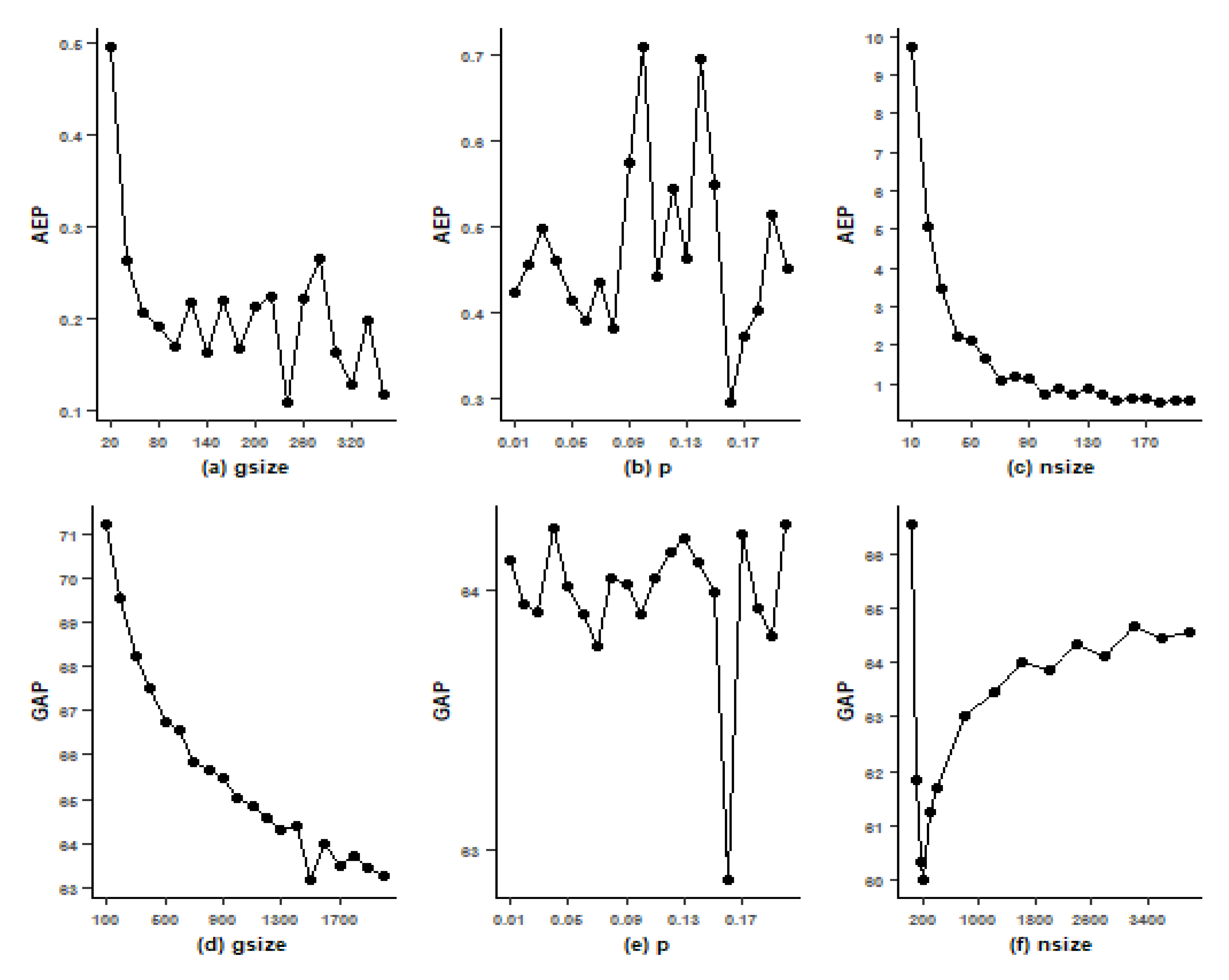
• Step 1. Initialize parameters: Set the values of n_size (number of parents), P_m (mutation rate), and g_size (number of iterations);
• Step 2. Generate an initial population of n_size parents (schedules) and evaluate their fitness values;
• Step 3. Iterate i from 1 to g_size:

-

Select two parents from the population using the roulette wheel method;

-

Apply linear order crossover to produce a set of n_size offspring;

-

For each offspring, generate a random number r (0 < r < 1). If r is less than P_m, perform a displacement mutation to create a new offspring;

-

Keep track of the best schedule found so far;

-

Replace the current population of parents with their offspring;

• Step 4. End the iteration loop (g_size);
• Step 5. Output the final best schedule and its corresponding fitness value.

By following these steps, the GA gradually evolves a population of schedules over multiple iterations, utilizing crossover and mutation operators to explore the search space and improve the quality of the solutions. The algorithm terminates after reaching the specified number of iterations, providing the best schedule found and its associated fitness value as the output.

5. The Parameter Exploration for GA

In this section, two different values of n are utilized for parameter exploration of GA: a large n = 400 and a small n = 10. Additionally, the learning dates control parameters for both machines, denoted as w₁ and w₂, are set to 0.5. For the scenarios with large n = 400 and small n = 10, one hundred instances are generated for each case. Data analysis is conducted for each dataset, involving the processing times $u_{1i}$ and $u_{2i}$ of jobs on machine M₁ and machine M₂, respectively. These times are uniformly distributed within the range U(51, 100). Under the influence of learning effect, the processing times $v_{1i}$ and $v_{2i}$ for jobs on machine M₁ and machine M₂ are generated from U(1, 50). The learning dates ${LD}_1$ and ${LD}_2$ for machine M₁ and machine M₂ are derived from U(1, U(1, $w_1{\sum }_{i=1}^n{u}_{1i}$)) and U(1, $w_2{\sum }_{i=1}^n{u}_{2i}$), respectively.

In this data context, we compute both the optimal solutions (Oi) obtained through the branch-and-bound method and the approximate solutions (Hi) obtained using the genetic algorithm (GA). The average error percentage (AEP) is calculated as A AEP = $\left\{{\sum }_1^{100}\left(Hi-Oi\right)/Oi\right\}\times 100\%$ to investigate the simulated parameter combinations (such as evolution generations Gsize, mutation rate p, and chromosome count n_size) within the GA algorithm. The experimental approach entails initially fixing two parameters and then varying the third parameter as the experimental subject for testing and exploration. This process continues until the minimum AEP value is identified. The parameter is then treated as a fixed parameter, and the aforementioned method is applied to identify the next suitable parameter. This iterative process persists until appropriate values are determined for all parameters.

First, the scenario with n = 10 was tested. Figure 1a depicts the parameter exploration of evolution generations (g_size) under the condition of a fixed mutation rate of p = 0.02 and a chromosome count of n_size = 500. The g_size was varied from 20 to 360, with increments of 20 generations. From Figure 1a, it is evident that the lowest point of the average error percentage (AEP) was reached at 240 generations. Therefore, 240 generations was selected as the value for the g_size for subsequent simulation testing.

Based on the above findings, the optimal number of evolution generations was determined to be 240. Therefore, with the evolution generations fixed at g_size = 240 and the mutation rate at p = 0.02, we conducted an exploration of the chromosome count parameter (n_size). Specifically, we varied the chromosome count (n_size) from a minimum of 10 chromosomes to a maximum of 200 chromosomes, increasing by 10 chromosomes in each step. In Figure 1b, it can be observed that the GA reached a relatively stable state around 100 chromosomes. However, the lowest point occurred at 180 chromosomes. Hence, we selected 180 chromosomes as the reference value for the n_size in the subsequent GA simulation testing.

Based on the results above, we determined that suitable values were g_size = 240 for evolution generations and n_size = 180 for chromosome count. Therefore, in the subsequent steps, we fixed g_size = 240 and n_size = 180 to explore the parameter range of mutation rate (p). We considered a mutation rate range from 0.01 to 0.2, with increments of 0.01. As evident from Figure 1c, it became evident that the GA achieved the minimum error at a mutation rate of 0.16. Consequently, this study employed a mutation rate of 0.16 as the basis for GA testing in the subsequent phases.

Next, the initial setup for parameter exploration involving a larger n was conducted with n = 400. The branch-and-bound method was utilized to calculate the root lower bound value (LBi), and the genetic algorithm (GA) was used to compute approximate solutions (Hi). The percentage gap in their differences (average gap percentage or GAP) was computed as GAP = $\left\{{\sum }_1^{100}\left(Hi-LBi\right)/LBi\right\}\times 100\%$ to explore the parameter values of g_size (evolution generations), p (mutation rate), and n_size (chromosome count) for the GA. The goal was to determine the optimal values of g_size, p, and n_size that yielded the most suitable GAP values. These optimal values were intended for reference in subsequent GA algorithm simulations for larger n.

As shown in Figure 1d, when n = 400, with n_size = 2000 fixed and a mutation rate of p = 0.02, the exploration of the evolution generations (g_size) ranges from a minimum of 100 generations to a maximum of 2000 generations, increasing by 100 generations in each step. From the graph, it is evident that the lowest GAP value occurred at around 1500 generations. Consequently, the evolution generations for the subsequent GA simulations was set to g_size = 1500.

Subsequently, the exploration of the mutation rate was conducted with n = 400, g_size = 1500, and n_size = 2000 held constant. The range of mutation rates for investigation was set from 0.01 to 0.2, increasing by increments of 0.01. From Figure 1e, it becomes evident that the mutation rate p reached its lowest GAP value at 0.16. Therefore, the subsequent GA algorithm adopted a mutation rate setting of p = 0.16.

Finally, with n = 400, g_size = 1500, and p = 0.16 fixed, we explored the parameter n_size (chromosome count). Figure 1f illustrates that when setting the chromosome count from 400 to 4000, with increments of 400 chromosomes in each step for simulation testing, the results indicated a progressively increasing trend in GAP values. Consequently, we considered an exploration range for an n_size between 100 and 400 chromosomes, increasing by 100 chromosomes in each step. Additionally, we also assessed the performance of GA with a chromosome count of 50. Observing the graph, it is apparent that the lowest GAP value occurred at a chromosome count of 200. Therefore, the decision was taken to utilize 200 chromosomes as the parameter for subsequent GA testing.

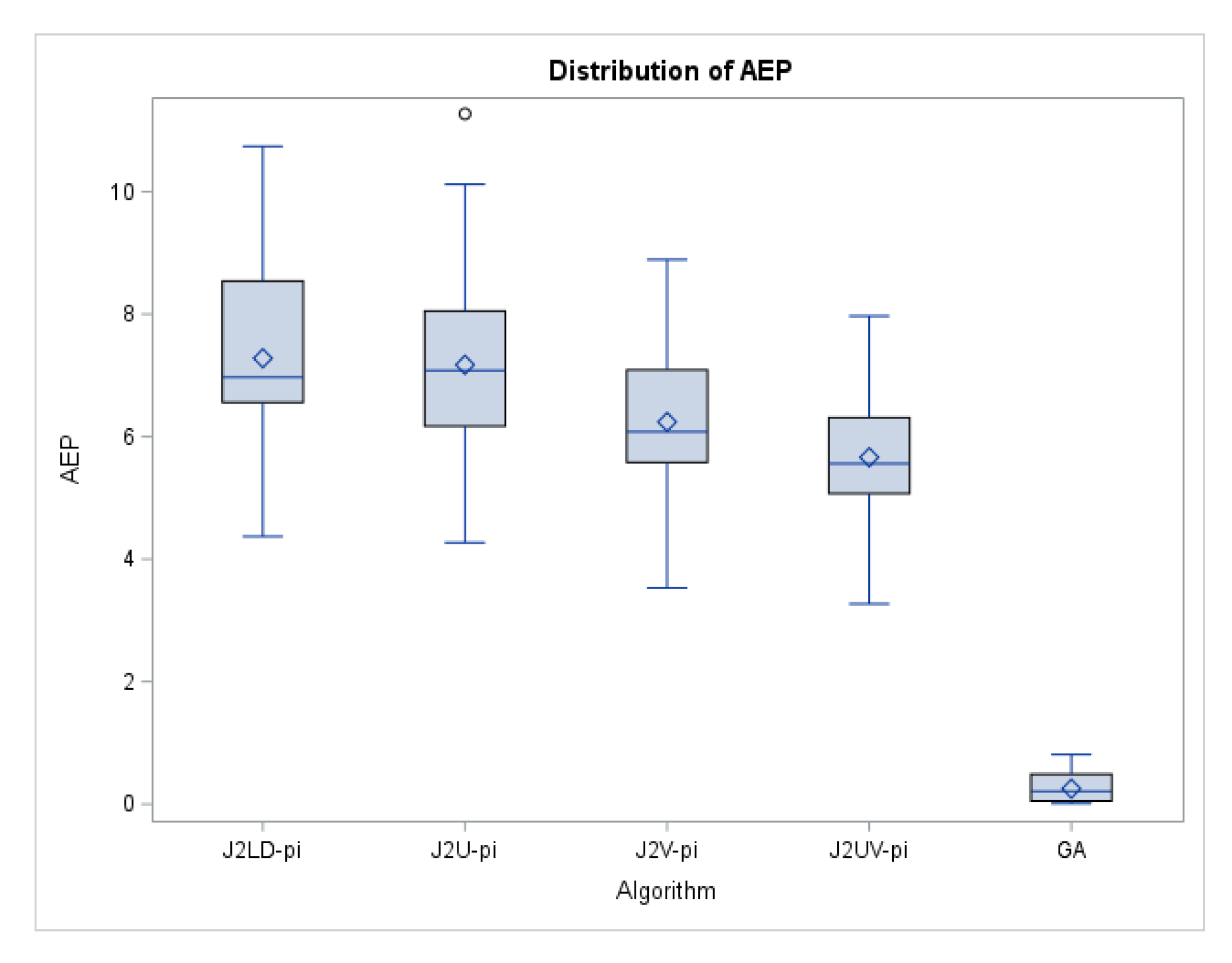
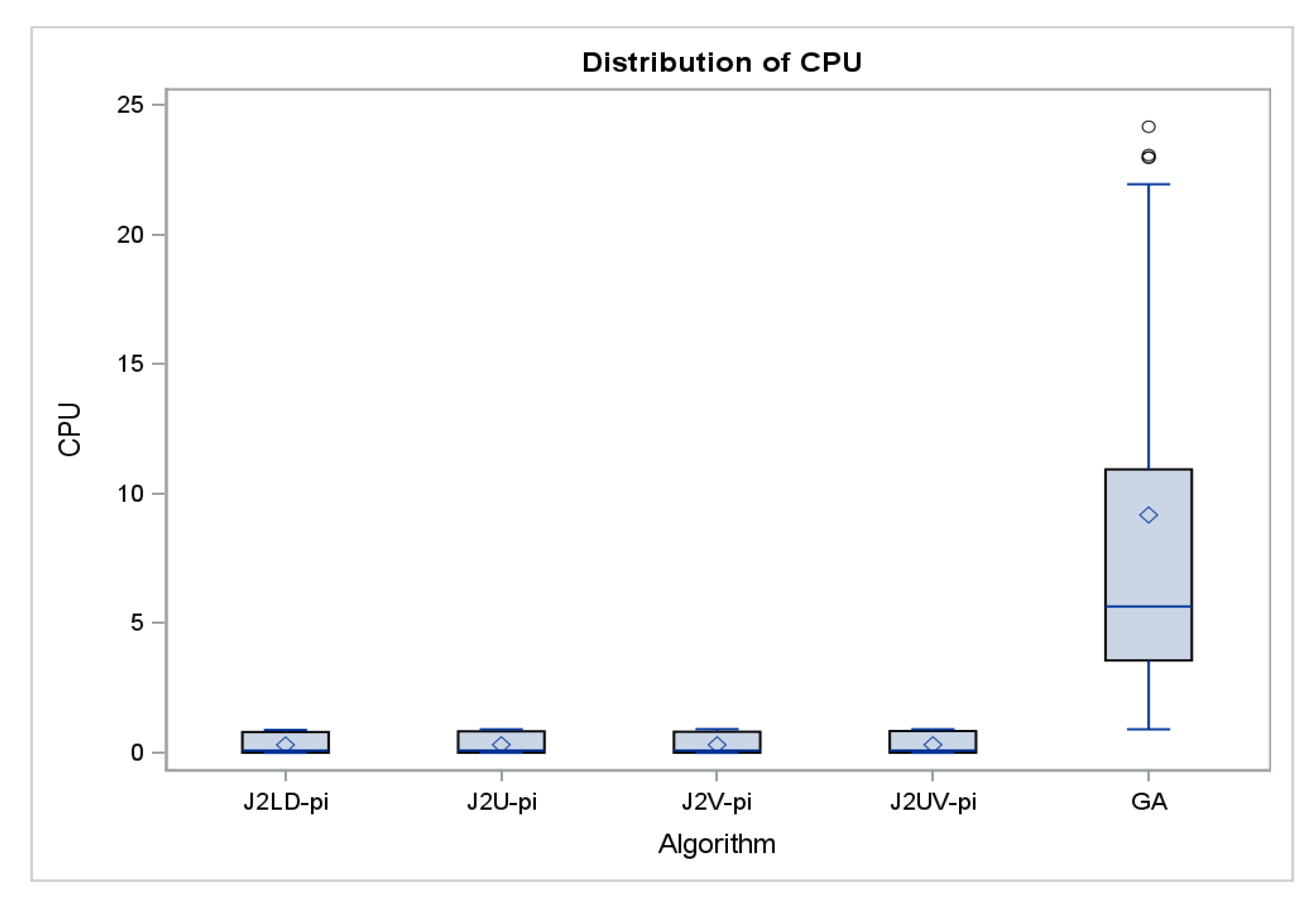
6. Simulation Results for Proposed Algorithms

In this section, we conducted several experimental designs to evaluate the performances of the four proposed algorithms, a population-based genetic algorithm, and a branch-and-bound method. The designs included six different values of n with n = 8, 10, and 12 for the small number of jobs and n = 100, 200, and 400 for the big number of jobs, along with nine cases of learning date control parameters (w₁, w₂) with (0.25, 0.25), (0.25, 0.5), (0.25,0.75), (0.5, 0.25), (0.5, 0.5), (0.5,0.75), (0.75, 0.25), (0.75, 0.5), and (0.75,0.75). For each case, the processing times $u_{1i}$ and $u_{2i}$ of jobs on machine M₁ and machine M₂ were generated from within the range U(51, 100), uniformly distributed, respectively. Meanwhile, under the influence of learning effect, the processing times $v_{1i}$ and $v_{2i}$ for jobs on machine M₁ and machine M₂ were generated from U(1, 50), respectively. Additionally, the learning dates ${LD}_1$ and ${LD}_2$ for machine M₁ and machine M₂ were derived from U(1, U(1, $w_1{\sum }_{i=1}^n{u}_{1i}$)) and U(1, $w_2{\sum }_{i=1}^n{u}_{2i}$), respectively. This study reports 54 cases and one hundred instances for each case. In total, we generated 5400 tested instance problems where 2700 instances were for the small number of jobs and for the big number of jobs, respectively. The results of six different values of n with n = 8, 10, and 12 for the small number of jobs and n = 100, 200, and 400 for the big number of jobs are reported in

Table 2. The performance of four heuristics and GA on the small number of jobs.

n	${\mathit{w}}_1$	${\mathit{w}}_2$	BB		J2LD-pi		J2U-pi		J2V-pi		J2UV-pi		GA
			mean	max	mean	sd	mean	sd	mean	sd	mean	sd	mean	sd
8	0.25	0.25	10	146	9.41	7.43	8.65	7.21	6.41	6.55	5.56	4.76	0.01	0.08
		0.50	1298	7649	7.21	6.11	6.63	5.48	5.40	5.36	5.22	4.70	0.03	0.18
		0.75	5075	19594	4.37	4.66	4.27	4.84	3.54	4.16	3.27	4.28	0.00	0.03
	0.50	0.25	206	3171	6.82	5.33	7.08	5.86	6.71	5.72	5.86	5.02	0.07	0.37
		0.50	89.63	1025	7.56	5.30	7.45	5.02	5.85	4.40	5.33	4.06	0.04	0.19
		0.75	3727	19,875	4.71	5.25	4.78	4.87	3.53	3.66	3.63	3.52	0.03	0.23
	0.75	0.25	1466	11,481	5.30	4.76	5.59	4.82	4.77	5.1	4.39	4.85	0.04	0.30
		0.50	1090	8064	6.69	5.12	6.17	4.56	5.82	4.34	5.07	4.26	0.06	0.26
		0.75	2610	12,331	4.70	4.51	4.93	4.24	4.50	4.04	4.08	3.97	0.05	0.28
10	0.25	0.25	48	3428.00	6.27	5.83	7.13	5.61	7.09	5.92	5.53	5.12	0.21	0.75
		0.50	2499	41,120.00	9.77	5.84	10.12	6.37	6.6	4.44	5.82	4.55	0.17	0.41
		0.75	49,700	424,496	7.93	5.37	8.54	5.78	5.65	4.69	5.38	4.47	0.13	0.48
	0.50	0.25	4752	91,532	8.07	5.58	7.60	4.70	8.02	5.41	6.57	4.24	0.28	0.77
		0.50	2580	44,931	8.90	5.09	9.00	4.83	7.65	4.48	6.87	4.41	0.54	1.04
		0.75	44,392	486,987	7.06	4.52	7.56	4.78	5.68	4.57	4.90	3.79	0.22	0.69
	0.75	0.25	76,650	533,020	4.97	4.25	5.37	4.79	5.42	4.57	4.82	4.49	0.18	0.53
		0.50	38,918	387,621	6.56	4.75	5.75	4.62	5.67	4.40	5.59	4.41	0.23	0.64
		0.75	31,791	176,396	6.81	4.92	6.18	4.35	5.58	3.83	5.56	4.11	0.23	0.62
12	0.25	0.25	129	11,366	6.76	4.89	6.98	5.07	7.13	5.50	6.19	4.99	0.21	0.55
		0.50	170,353	7,713,811	10.74	5.71	11.27	5.59	8.31	5.17	7.43	5.09	0.52	0.99
		0.75	5,014,307	77699120	7.87	5.48	7.45	4.91	5.96	4.58	5.89	3.95	0.19	0.57
	0.50	0.25	122,303	1,916,426	8.62	5.06	8.05	4.73	8.89	5.10	7.73	4.39	0.61	1.15
		0.50	48,587	2,792,148	10.09	5.73	9.17	4.60	8.49	4.08	7.97	4.01	0.81	0.96
		0.75	1,363,555	16,993,648	8.54	4.61	7.70	5.01	6.49	4.52	6.34	4.17	0.39	0.74
	0.75	0.25	3,589,247	32,696,624	5.70	4.88	5.52	4.04	6.45	5.58	5.59	4.73	0.37	0.84
		0.50	1,590,399	19,702,024	6.88	4.95	6.90	5.06	6.08	4.44	5.26	4.14	0.53	0.93
		0.75	1,941,574	43,576,680	6.97	4.21	6.68	4.74	6.62	3.50	6.31	4.44	0.49	0.99
	mean		522494		7.23		7.13		6.23	5.63			0.25

and

Table 3. The performance of four heuristics and GA on the big number of jobs.

n	${\mathit{w}}_1$	${\mathit{w}}_2$	J2LD_pi		J2U-pi		J2V-pi		J2UV-pi		GA
			mean	sd	mean	sd	mean	sd	mean	sd	mean	sd
100	0.25	0.25	5.91	3.18	5.94	2.71	6.86	2.64	6.16	2.5	0.03	0.21
		0.5	13.26	3.44	11.5	3.67	10.54	3.34	8.87	2.76	0.00	0.00
		0.75	10.96	4.74	9.82	4.35	9.24	4.06	7.56	3.66	0.00	0.00
	0.50	0.25	11.04	3.44	10.1	2.97	12.72	3.10	11.72	3.83	0.00	0.00
		0.5	9.05	3.65	7.74	2.68	8.32	3.03	7.71	2.39	0.00	0.00
		0.75	12.00	4.14	9.68	4.05	8.25	3.97	7.58	3.37	0.00	0.00
	0.75	0.25	9.71	4.25	8.25	3.59	12.09	4.76	9.69	3.86	0.00	0.00
		0.5	9.76	4.97	7.31	3.25	10.6	4.22	9.33	4.81	0.00	0.00
		0.75	7.42	3.18	5.97	3.13	4.81	2.83	5.19	2.97	0.00	0.00
200	0.25	0.25	2.58	1.89	2.29	1.84	3.33	2.00	2.99	1.88	0.41	0.77
		0.5	10.96	2.95	10.00	2.85	8.64	3.000	6.61	2.66	0.00	0.00
		0.75	10.33	3.80	10.81	3.86	9.59	3.22	8.16	2.69	0.00	0.00
	0.50	0.25	9.88	2.81	8.57	2.48	11.51	2.56	10.24	2.65	0.00	0.00
		0.5	6.33	3.24	4.15	2.01	5.37	2.26	4.49	1.95	0.03	0.15
		0.75	11.91	4.12	10.1	4.48	8.53	3.12	7.8	2.63	0.01	0.05
	0.75	0.25	11.39	5.49	7.21	3.04	12.13	4.19	9.99	3.97	0.00	0.00
		0.5	11.02	4.88	7.76	3.36	11.98	4.72	9.08	3.64	0.00	0.00
		0.75	9.08	4.53	5.87	3.34	8.30	3.05	6.20	2.62	0.01	0.13
400	0.25	0.25	1.15	1.38	1.03	1.09	1.67	1.6	1.71	1.52	2.48	1.14
		0.50	6.91	1.96	6.18	1.86	5.19	1.87	2.83	1.51	0.01	0.06
		0.75	10.09	3.53	10.08	3.82	7.73	2.57	6.02	2.56	0.00	0.00
	0.50	0.25	3.92	1.94	3.21	1.67	6.20	1.82	4.67	1.55	0.06	0.32
		0.50	3.63	2.21	1.44	1.21	3.92	1.63	2.35	1.38	0.29	0.59
		0.75	10.52	3.91	9.52	3.16	6.98	2.56	5.54	2.28	0.02	0.19
	0.75	0.25	8.36	3.52	6.91	3.08	12.49	3.41	9.31	3.08	0.00	0.03
		0.50	9.66	4.36	6.47	2.97	11.87	3.85	8.92	3.81	0.01	0.07
		0.75	6.71	5.30	3.49	2.95	6.16	3.34	4.09	2.59	0.37	0.74
	mean		8.65		7.01		8.34		6.84		0.14

.

For the cases of the small number of jobs, we computed both the optimal solutions (Oi) obtained through the branch-and-bound method (B&B) and the approximate solutions (Hi) obtained using the four heuristics (J2LD-pi, J2U-pi, J2V-pi, J2UV-pi) and genetic algorithm (GA). The average error percentage (AEP) was calculated as AEP=$\left\{{\sum }_1^{100}\left(Hi-Oi\right)/Oi\right\}\times 100\%$ and standard deviation (STD) of errors to determine the performances of all the proposed algorithms over the different values of n, w₁, and w₂. Regarding the performance of B&B, we reported the mean and maximum of explored nodes and their corresponding CPU time (in second) for each case. Additionally, we designed a tested instance problem as not feasible one when the B&B consumed the number of nodes up to ${10}^9$. The effects of n, w_1, and w₂ in

Table 4. The summary performance of B&B.

		Node	CPU-Time
n	w1	mean	mean
8	0.25	6385	0.0242
	0.50	4023	0.0117
	0.75	5167	0.0124
	w2
	0.25	1684	0.0060
	0.50	2478	0.0061
	0.75	11,413	0.0362
	w1
10	0.25	52,248	0.1625
	0.50	51,725	0.1832
	0.75	147,360	0.5204
	w2
	0.25	81,451	0.2823
	0.50	43,997	0.1530
	0.75	125,884	0.4308
	w1
12	0.25	5,184,789	25.1863
	0.50	1,534,446	7.4038
	0.75	7,121,221	34.8778
	w2
	0.25	3,711,680	17.6078
	0.5	1,809,341	8.8510
	0.75	8,319,437	41.0091

and

Table 5. The summary AEP performance of proposed algorithms for small n.

		J2LD-pi	J2U-pi	J2V-pi	J2UV-pi	GA
n	w1	mean	mean	mean	mean	mean
8	0.25	7.00	6.52	5.12	4.68	0.01
	0.50	6.36	6.44	5.36	4.94	0.05
	0.75	5.56	5.56	5.03	4.51	0.05
	w2
	0.25	7.18	7.11	5.96	5.27	0.04
	0.50	7.15	6.75	5.69	5.21	0.04
	0.75	4.59	4.66	3.86	3.66	0.03
	w1
10	0.25	7.99	8.60	6.45	5.58	0.17
	0.50	8.01	8.05	7.12	6.11	0.35
	0.75	6.11	5.77	5.56	5.32	0.21
	w2
	0.25	6.44	6.70	6.84	5.64	0.22
	0.50	8.41	8.29	6.64	6.09	0.31
	0.75	7.27	7.43	5.64	5.28	0.19
	w1
12	0.25	8.46	8.57	7.13	6.50	0.31
	0.50	9.08	8.31	7.96	7.35	0.60
	0.75	6.52	6.37	6.38	5.72	0.50
	w2
	0.25	7.03	6.85	7.49	6.50	0.44
	0.5	9.24	9.11	7.63	6.89	0.62
	0.75	7.79	7.28	6.36	6.18	0.36
	n
	8	6.31	6.17	5.17	4.71	0.04
	10	7.37	7.47	6.37	5.67	0.24
	12	8.02	7.75	7.16	6.52	0.47
	mean	7.23	7.13	6.23	5.64	0.25

were obtained from Table 2.

For the performance of B&B, Table 4 shows that B&B took more nodes at $w_2=0.75$ than those at $w_2=0.25$ or 0.5. The pattern of $w_1$ was similar to that of $w_2$, except n = 8. The pattern became clear as n increases. It also can be observed in Table 2 that B&B consumed fewer nodes at $w_1=0.5$ or $w_2=0.5$. We also noted that in the two cases of n = 10, with different weight configurations $w_1$ = 0.25 and $w_1$ = 0.5, although the total mean node count was higher in the case of $w_1$ = 0.25, this is because in this case, the maximum node count for the weight configuration ($w$ = 0.5, $w_2$ = 0.75) was even greater than the maximum node count for ($w_1$ = 0.25, $w_2$ = 0.75). However, the time taken to solve these two scenarios was remarkably similar. This is why, in the scenario with $w_1$ = 0.25, despite having a higher total mean node count, the time required to solve the problem was less. Overall, the nodes grew very large as n increased. It can be confirmed this problem is an NP-hard one.

With respect to the achieved results of the four proposed heuristics and the genetic algorithm (GA) applied to the case of small n, Table 5 and Figure 2 illustrate their AEPs. In summary, the mean AEP values were 7.23, 7.13, 6.23, 5.64, and 0.25 for J2LD_pi, J2U_pi, J2V_pi, J2UV_pi, and GA, respectively. It is evident that the GA algorithm outperformed all of the other four heuristics.

Table 5 further presents the means of AEP values corresponding to different levels of the factors n, $w_1$, and $w_2$. An observation from Table 5 revealed that the AEPs of the four heuristics and the GA algorithm exhibited a slight increase as n increased from 8 to 12. Conversely, these AEPs remained relatively unaffected by variations in the values of $w_1$ or $w_2$. Turning to the computational times, Figure 3 demonstrates that all four heuristics and the GA algorithm required less than 1 s to execute.

Statistical evidence to determine the significance of differences among the four heuristics and the GA algorithm is discussed below. Initially, an analysis of variance (ANOVA) method using a linear model was employed on the AEP data within SAS 9.4. However, the normality assumption of the linear model was found to be violated. This was evident from the Kolmogorov–Smirnov normality test, which yielded a p-value less than 0.05 (with a statistic value of 0.084). Consequently, due to this non-normality, the data were handled using a nonparametric approach. Specifically, for the 32 instances of the (n*w₁*w₂) problem, the Friedman test (with p-value less than 0.0001) was conducted based on ranks of AEP values. The results of the test provided evidence that the AEP samples were not drawn from the same distribution at a significance level of α = 0.05.

To further assess $\left(\begin{array}{c}5\\ 2\end{array}\right)$ pairwise differences among the four heuristics and the GA algorithm, the WNMT (Wilcoxon–Nemenyi–McDonald–Thompson) procedure was introduced.

Table 6. The summary RPD performance of proposed algorithms for big n.

		J2LD-pi	J2U-pi	J2V-pi	J2UV-pi	GA
n	w1	mean	mean	mean	mean	mean
100	0.25	10.04	9.09	8.88	7.53	0.01
	0.50	10.7	9.17	9.76	9.00	0.00
	0.75	8.96	7.18	9.17	8.07	0.00
	w2
	0.25	8.89	8.1	10.56	9.19	0.01
	0.50	10.69	8.85	9.82	8.64	0.00
	0.75	10.13	8.49	7.43	6.78	0.00
	w1
200	0.25	7.96	7.7	7.19	5.92	0.14
	0.50	9.37	7.61	8.47	7.51	0.01
	0.75	10.5	6.95	10.8	8.42	0.00
	w2
	0.25	7.95	6.02	8.99	7.74	0.14
	0.50	9.44	7.3	8.66	6.73	0.01
	0.75	10.44	8.93	8.81	7.39	0.01
	w1
400	0.25	0.25	6.05	5.76	4.86	3.52
	0.50	0.50	6.02	4.72	5.7	4.19
	0.75	0.75	8.24	5.62	10.17	7.44
	w2
	0.25	0.25	4.48	3.72	6.79	5.23
	0.5	0.5	6.73	4.70	6.99	4.70
	0.75	0.75	9.11	7.70	6.96	5.22
	n
	100	9.90	8.48	9.27	8.20	0.00
	200	9.28	7.42	8.82	7.28	0.05
	400	6.77	5.37	6.91	5.05	0.36
	mean	8.65	7.09	8.33	6.84	0.14

(column 3) illustrates the sum of ranks of AEP for the 32 instance problems across the four heuristics and the GA algorithm. The rank sums for J2LD_pi, J2U_pi, J2V_pi, J2UV_pi, and GA were 118, 117, 88, 55, and 27, respectively. Statistically, there was no significant difference among the groups of J2LD_pi, J2U_pi, and J2V_pi at a significance level of 0.05. However, J2UV_pi demonstrated a significant improvement over each of the J2LD_pi, J2U_pi, and J2V_pi heuristics. Additionally, the GA algorithm exhibited significant superiority compared to each of the J2LD_pi, J2U_pi, J2V_pi, and J2UV_pi heuristics. Notably, the GA yielded the smallest AEP and rank sum for a small number of jobs.

Concerning the obtained results in Table 3 for the proposed four heuristics and the GA algorithm in the context of large n, Table 6 (summarized from Table 3) and Figure 4 provide an account of the average Relative Percentage Deviation (RPD) for the four heuristics and the GA algorithm. It is evident from

Table 7. The sum of ranks for four heuristics and GA algorithm.

Heuristic/Algorithm	No. of Obs./Small n	Rank-Sum (Ri, i = 1, 2,…, 5)	No. of Obs./Large n	Rank-Sum (Ri, i = 1, 2, …, 5)
J2LD-pi	27	118	27	112
J2U-pi	27	117	27	76
J2V-pi	27	88	27	108
J2UV-pi	27	55	27	78
GA	27	27	27	31

The WNMT test indicates that two algorithms are significantly different if |Ri-Rj| > 32, for both small n and large n approximately.

that, regardless of the value of n, the GA consistently achieved the lowest average RPD among all job sequences. The average RPD values for J2LD_pi, J2U_pi, J2V_pi, J2UV_pi, and GA were 8.65, 7.09, 8.33, 6.84, and 0.14, respectively. Furthermore, Figure 4 presents box plots depicting the distribution of average RPD for both the four heuristics and the GA algorithm. These box plots indicate that the interquartile ranges of average RPDs for J2LD_pi, J2U_pi, J2V_pi, and J2UV_pi in comparison to the GA algorithm were broader. It is also noteworthy from Table 3 that as the value of n increased from 100 to 400, the average RPD values of J2LD_pi, J2U_pi, J2V_pi, and J2UV_pi decreased. Conversely, the average RPD of the GA algorithm experienced only a slight increase.

A linear model was applied to the average RPD observations in order to analyze the distinctions between the four heuristics and a GA algorithm. Nevertheless, the assumption of normality for the RPD samples was violated, as indicated by p-values lower than 0.05 in the Kolmogorov–Smirnov normality test. The calculated statistic was 0.096. Consequently, the Friedman’s test with a chi-square value of 69.1532 (p-value of less than 0.0001) was employed to explore the pairwise variations among all proposed algorithms. Examining the sum of ranks of the average RPD computed for each of the 27 blocks related to the test problem instances, these outcomes validated that the average RPD samples did not adhere to the same distribution. In other words, J2LD_pi, J2U_pi, J2V_pi, J2UV_pi, and GA exhibited distinct search performances.

Table 7 (column 5) displays the rank-sum of average RPDs for J2LD_pi, J2U_pi, J2V_pi, J2UV_pi, and GA. To conduct a more detailed comparison of ($\genfrac{}{}{0pt}{}{5}{2}$) pairwise differences among 2LD_pi, J2U_pi, J2V_pi, J2UV_pi, and GA, the WNMT test (with a significance level of 0.05) was employed. The results indicated that GA achieved the best performance, being placed in the group with the lowest rank-sum of 31. On the other hand, the heuristics (J2LD_pi, J2U_pi, J2V_pi, J2UV_pi) were categorized in the group with higher rank-sums (76, 112), implying inferior performance. This test confirmed that, at a significance level of α = 0.05, the GA algorithm statistically outperformed each of the four heuristics individually. Overall, the GA algorithm demonstrated the most effective search capability, particularly for scenarios involving a large number of jobs.

Regarding computational time, Figure 5 displays the box plots of CPU times (in seconds) for the five proposed algorithms. On average, the GA algorithm required a mean CPU time of 10.36 s to solve an instance problem, whereas each of the J2LD_pi, J2U_pi, J2V_pi, and J2UV_pi heuristics necessitated an average CPU time of 0.32 s to solve an instance problem. This discrepancy in CPU time can be attributed to the heightened computational demands of the GA algorithm when compared to each of the J2LD_pi, J2U_pi, J2V_pi, and J2UV_pi heuristics. The underlying factors contributing to the increased CPU time for GA include its elevated complexity, the need for diversity maintenance, adaptation, global search, and problem-specific techniques intrinsic to metaheuristic approaches.

7. Conclusions and Suggestions

This study delved into the scheduling of the two-machine flow-shop problem using step-learning. In this context, job processing times decrease if they commence after their job-dependent learning dates. Initially, we concentrated on a scenario where there was no allowance for idle time between successive jobs on the first machine, yet idle periods were permissible on the second machine. The main goal of this investigation was to optimize resource allocation and task sequencing, aiming to maximize time utilization efficiency and ensure the timely completion of all jobs, a shared objective in the pursuit of scheduling process optimization.

For this challenging problem, we proposed a Mixed-Integer Programming (MIP) model. Subsequently, we employed a branch-and-bound method with two dominance properties and a lower bound to generate optimal solutions for cases with a small number of jobs (e.g., n = 8, 10, and 12). This method performed well up to n = 12 jobs, which encompassed various combinations of job classes and controllable learning indices w₁ and w₂ for learning dates. For cases with a larger number of jobs, such as n = 100, 200, and 400, we introduced four problem-based heuristics, each accompanied by a pairwise interchange scheme, along with a genetic algorithm (GA) for obtaining approximate solutions. It was observed that the GA outperformed the other four heuristics in both small n and large n tested instances.

One of the issues for future study is to expand the production environment to a two-stage three-machine flow-shop production process with learning dates. Additionally, it is worthwhile to consider extending the same setup to minimize the total completion times of all provided jobs.

References

1. Bottou, L. Stochastic gradient descent tricks. In Neural Networks: Tricks of the Trade; Springer: Berlin/Heidelberg, Germany, 2012; pp. 421–436. [Google Scholar]
2. Goodfellow, I.; Bengio, Y.; Courville, A. Deep Learning; MIT Press: Cambridge, MA, USA, 2016. [Google Scholar]
3. Pinedo, M. Scheduling: Theory, Algorithms, and Systems; Springer Science & Business Media: Berlin, Germany, 2012. [Google Scholar]
4. Ruder, S. An overview of gradient descent optimization algorithms. arXiv 2016, arXiv:1609.04747. [Google Scholar]
5. Russell, S.J.; Norvig, P. Artificial Intelligence: A Modern Approach; Prentice Hall: Hoboken, NJ, USA, 2010. [Google Scholar]
6. Biskup, D. Single-machine scheduling with learning considerations. Eur. J. Oper. Res. 1999, 115, 173–178. [Google Scholar] [CrossRef]
7. Cheng TC, E.; Wang, G. Single machine scheduling with learning effect considerations. Ann. Oper. Res. 2000, 98, 273–290. [Google Scholar] [CrossRef]
8. Kuo, W.H.; Yang, D.L. Minimizing the total completion time in a single- machine scheduling problem with a time- dependent learning effect. Eur. J. Oper. Res. 2006, 174, 1184–1190. [Google Scholar] [CrossRef]
9. Koulamas, C.; Kyparisis, G.J. Single-machine and two-machine flowshop scheduling with general learning functions. Eur. J. Oper. Res. 2007, 178, 402–407. [Google Scholar] [CrossRef]
10. Wang, J.B. Single-machine scheduling problems with the effects of learning and deterioration. Omega 2007, 35, 397–402. [Google Scholar] [CrossRef]
11. Yin, Y.; Xu, D.; Sun, K.; Li, H. Some scheduling problems with general position-dependent and time-dependent learning effects. Inf. Sci. 2009, 179, 2416–2425. [Google Scholar] [CrossRef]
12. Wu, C.-C.; Yin, Y.; Cheng, S.-R. Some single-machine scheduling problems with a truncation learning effect. Comput. Ind. Eng. 2011, 60, 790–795. [Google Scholar] [CrossRef]
13. Wu, C.-C.; Yin, Y.; Wu, W.-H.; Cheng, S.-R. Some polynomial solvable single-machine scheduling problems with a truncation sum-of-processing-times based learning effect. Eur. J. Ind. Eng. 2012, 6, 441–453. [Google Scholar] [CrossRef]
14. Wu, C.-C.; Yin, Y.; Cheng, S.-R. Single-machine and two-machine flowshop scheduling problems with truncated position-based learning functions. J. Oper. Res. Soc. 2013, 64, 147–156. [Google Scholar] [CrossRef]
15. Wang, J.B.; Wang, J.-J. Single machine scheduling with sum-of-logarithm- processing-times based and position based learning effects. Optim. Lett. 2014, 8, 971–982. [Google Scholar] [CrossRef]
16. Niu, Y.-P.; Wan, L.; Wang, J.-B. A Note on Scheduling Jobs with Extended Sum-of-Processing-Times-Based and Position-Based Learning Effect. Asia Pac. J. Oper. Res. 2015, 32, 1550001. [Google Scholar] [CrossRef]
17. Zhang, X.; Liu, S.C.; Yin, Y.; Wu, C.-C. Single-machine scheduling problems with a learning effect matrix. Iranian Journal of Science and Technology. Trans. A Sci. 2018, 42, 1327–1335. [Google Scholar]
18. Biskup, D. A state-of-the-art review on scheduling with learning effect. Eur. J. Oper. Res. 2008, 188, 315–329. [Google Scholar] [CrossRef]
19. Janiak, A.; Krysiak, T.; Trela, R. Scheduling problems with learning and ageing effects: A survey. Decis. Mak. Manuf. 2011, 5, 19–36. [Google Scholar] [CrossRef]
20. Azzouz, A.; Ennigrou, M.; Ben Said, L. Scheduling problems under learning effects: Classification and cartography. Int. J. Prod. Res. 2018, 56, 1642–1661. [Google Scholar] [CrossRef]
21. Wang, J.B.; Xia, Z.Q. Flow-shop scheduling with a learning effect. J. Oper. Res. Soc. 2005, 56, 1325–1330. [Google Scholar] [CrossRef]
22. Xu, Z.; Sun, L.; Gong, J. Worst-case analysis for flow shop scheduling with a learning effect. Int. J. Prod. Econ. 2008, 113, 748–753. [Google Scholar] [CrossRef]
23. Wu, C.C.; Wu, W.H.; Hsu, P.H.; Lai, K. A two-machine flowshop scheduling problem with a truction sunm of processing-times-based learning function. Appl. Math. Model. 2012, 36, 5001–5014. [Google Scholar] [CrossRef]
24. Wang, J.B.; Wang, M.Z. Worst-Case analysis for flow shop scheduling problems with an exponential learning effect. J. Oper. Res. Soc. 2012, 63, 130–137. [Google Scholar] [CrossRef]
25. Cheng, T.C.E.; Wu, C.C.; Chen, J.C.; Wu, W.H.; Cheng, S.R. Two-machine flowshop scheduling with a truncated learning function to minimize the makespan. Int. J. Prod. Econ. 2013, 141, 79–86. [Google Scholar] [CrossRef]
26. Wang, X.Y.; Zhou, Z.; Zhang, X.; Ji, P.; Wang, J.B. Several flowshop scheduling problems with truncated position-based learning effect. Comput. Oper. Res. 2013, 40, 2906–2929. [Google Scholar] [CrossRef]
27. Wang, J.B.; Liu, F.; Wang, J.J. Research on m-machine flow shop scheduling with truncated learning effects. Int. Trans. Oper. Res. 2019, 26, 1135–1151. [Google Scholar] [CrossRef]
28. Hsu, C.-L.; Lin, W.-C.; Duan, L.; Liao, J.-R.; Wu, C.-C.; Chen, J.-H. A robust two-machine flow-shop scheduling model with scenario-dependent processing times. Discret. Dyn. Nat. Soc. 2020, 2020, 3530701. [Google Scholar] [CrossRef]
29. Ho, M.H.; Hnaien, F.; Dugardin, F. Electricity cost minimisation for optimal makespan solution in flow shop scheduling under time-of-use tariffs. Int. J. Prod. Res. 2021, 59, 1041–1067. [Google Scholar] [CrossRef]
30. Lo, T.C.; Lin, B.M.T. Relocation scheduling in a two-machine flow shop with resource recycling operations. Mathematics 2021, 9, 1527. [Google Scholar] [CrossRef]
31. Chen, X.; Miao, Q.; Lin, B.M.T.; Sterna, M.; Blazewicz, J. Two-machine flow shop scheduling with a common due date to maximize total early work. Eur. J. Oper. Res. 2022, 300, 504–511. [Google Scholar] [CrossRef]
32. Choi, B.C.; Park, M.J. Two machine fowshop scheduling with convex resource consumption functions. Optim. Lett. 2023, 17, 1241–1259. [Google Scholar] [CrossRef]
33. Johnson, S.M. Optimal two- and three-stage production schedules with setup times. Nav. Res. Logist. Q. 1954, 1, 61–68. [Google Scholar] [CrossRef]
34. Holland, J. Adaptation in Natural and Artificial Systems; University of Michigan Press: Ann Arbor, MI, USA, 1975. [Google Scholar]
35. Essafi, I.; Matib, Y.; Dauzere-Peres, S. A genetic local search algorithm for minimizing total weighted tardiness in the job-shop scheduling problem. Comput. Oper. Res. 2008, 35, 2599–2616. [Google Scholar] [CrossRef]
36. Nguyen, S.; Mei, Y.; Zhang, M. Genetic programming for production scheduling: A survey with a unified framework. Complex Intell. Syst. 2017, 3, 41–66. [Google Scholar] [CrossRef]
37. Fan, J.; Zhang, C.; Liu, Q.; Shen, W.; Gao, L. An improved genetic algorithm for flexible job shop scheduling problem considering reconfigurable machine tools with limited auxiliary modules. J. Manuf. Syst. 2022, 62, 650–667. [Google Scholar] [CrossRef]
38. Tutumlu, B.; Saraç, T. A MIP model and a hybrid genetic algorithm for flexible job-shop scheduling problem with job-splitting. Comput. Oper. Res. 2023, 155, 10622. [Google Scholar] [CrossRef]
39. Wang, Y.C.; Chen, T. Adapted techniques of explainable artificial intelligence for explaining genetic algorithms on the example of job scheduling. Expert Syst. Appl. 2023, 234 Pt A, 1213769. [Google Scholar] [CrossRef]
40. Iyer, S.K.; Saxena, B.S. Improved memetic genetic algorithm for the permutation flowshop scheduling problem. Comput. Oper. Res. 2004, 31, 593–606. [Google Scholar] [CrossRef]
41. Wu, C.-C.; Wu, W.-H.; Chen, J.C.; Yin, Y.; Wu, W.-H. A study of the single-machine two-agent scheduling problem with release times. Appl. Soft Comput. 2013, 13, 998–1006. [Google Scholar] [CrossRef]
42. Larranaga, P.; Kuijpers, C.M.H.; Murga, R.H.; Inza, I.; Dizdarevic, S. Memetic genetic algorithms for the Travelling Salesman Problem: A Review of Representations and Operators. Artif. Intell. Rev. 1999, 13, 129–170. [Google Scholar] [CrossRef]
43. Kellegoz, T.; Toklu, B.; Wilson, J. Comparing efficiencies of genetic crossover operators for one machine total weighted tardiness problem. Appl. Math. Comput. 2008, 199, 590–598. [Google Scholar] [CrossRef]
44. Castelli, M.; Cattaneo, G.; Manzoni, L.; Vanneschi, L. A distance between populations for n-points crossover in memetic genetic algorithms. Swarm Evol. Comput. 2019, 44, 636–645. [Google Scholar] [CrossRef]
45. Nearchou, A.C. The effect of various operators on the genetic search for large scheduling problems. Int. J. Prod. Econ. 2004, 88, 191–203. [Google Scholar] [CrossRef]
Figure 1. The parameter exploration for GA on n = 10 and 400.
Mathematics 11 04060 g001
Figure 2. Violin plots of AEP for 4 heuristics and GA for small n.
Mathematics 11 04060 g002
Figure 3. Violin plots of CPU times for 4 heuristics and GA for small n.
Mathematics 11 04060 g003
Figure 4. The box plots of RPD for 4 heuristics and GA for big n.
Mathematics 11 04060 g004
Figure 5. The box plots of CPU times for 4 heuristics and GA for big n.
Mathematics 11 04060 g005