A Heuristic Model for Spare Parts Stocking Based on Markov Chains

Abstract

Spare parts management has gained significant attention in recent years due to the considerable costs associated with backorders or excess inventory. This article addresses the challenge of determining the optimal number of spare parts to stock, assuming that the parts can be repaired. When an item fails, it is promptly sent for repair in a workshop. The time between failures and the repair time are assumed to follow an exponential distribution, although it should be noted that the results could be adapted to other distributions as well. This study introduces a heuristic method to find the optimal inventory level that minimizes the total cost, considering holding inventory, backorder, and repair costs. The research offers a valuable decision-making framework for determining the number of spare parts needed to minimize inventory costs, based on just two parameters: (1) the ratio of time to repair and time to failure, and (2) the ratio of the inventory holding cost of a spare part per day to the daily cost of an idle machine. To the best of our knowledge, there are no similar methodologies in the existing literature. The proposed method is straightforward to implement, employing graphs and simple computations. Therefore, it is anticipated to be highly beneficial for practitioners seeking a quick and reliable estimator of the optimal number of spare parts to stock for critical components.

1. Introduction

The primary purpose of an inventory control policy is to optimize the total cost resulting from combining holding costs, ordering costs, and costs associated with shortages. In order to minimize these costs, inventory policies regularly provide answers to the questions: “What items should be stocked?”, “How much is the order quantity?”, and “How much of each item should be kept in stock?” [1]. Although inventory management is a common problem in most organizations, this does not mean that inventory control is a simple or easy problem to solve. Manufacturers keep a lot of raw materials, work-in-process, and finished goods in inventory. In addition, they also have a huge amount of inventories of equipment, machines, and spare parts, among other things. Many inventory models have been developed, the complexity of which depends on the assumptions the decision maker must consider about demand, the physical limitations of warehouses, or cost structure [2].

Within inventory systems, one research topic is related to spare parts. Spare parts inventories have a very different function from intermediate or final products, which must satisfy customer needs [3]. It has often been thought that spare parts inventories cannot be managed by traditional models or methods, since these inventories do not possess the conditions for their application. This is because the consumption pattern is sporadic (irregular and small), replenishment response times are long, and acquisition costs are high [4].

The management of spare parts inventories is essential to maintain the competitiveness of any company. In industrial plants, operating and maintenance costs account for more than 60% of overall costs [5], while costs related to spare parts alone account for 25–30%. Thus, correctly choosing the parts that must be in the spare parts inventory, establishing an order policy for these parts, and establishing a storage system for them greatly impacts the profitability and the equipment availability of a factory [6].

The importance of spare parts management is highlighted in [7,8] by using data on aircraft maintenance. Billions of dollars are spent on spare parts to reduce the expensive cost of idle aircraft, which can be as high as $100,000 per hour. If the needed part is not readily available, the engineer must place an order with the manufacturer of the aircraft with the associated and usually very high emergency ordering cost. A method to optimize maintenance parameters, motivated by significant savings, is proposed in [9]. The maintenance cost due to production interruption is minimized, contributing to reducing the total cost, which can be as high as 70% of the production cost.

Determining the optimal number of spare parts to keep is a difficult problem that involves several cost and distribution parameters. This research work proposes a methodology that, starting with five parameters, identifies the two most relevant ones that make it easy to find an optimal solution for the stated problem. In this paper, the context is that one or several machines have one important component whose failure may have catastrophic consequences if no spare part is available. When the component fails, the machine can be kept in operating condition if a spare component is available. The broken component is immediately taken to a maintenance shop for repair. If the newly installed component fails while the broken component is being repaired and no more spare parts are available, the machine stops, interrupting the operation and forcing emergency measures to be taken, with the corresponding extraordinarily high costs. Although keeping one spare part (like the spare tire in automobiles) may be enough, in some cases, especially when the cost of an idle machine is very high, it may be convenient to stock more than one spare component in inventory. However, having one or more spare components may also be costly if the failure rate of these components is low or if the consequences of failure are not important. This paper presents two related cases: one machine and several identical machines. The first case is found in almost every company, while the second is found, for example, in companies with several identical production/assembly lines and in transportation companies, which usually have several identical transport units.

The document is organized into five sections. Section 2 provides a literature review related to spare parts management, specifically focusing on the methods used to determine spare parts inventory strategies. Section 3 describes the construction of transition matrices for this problem, considering both single and multiple machine cases. In Section 4, the costs are analyzed, and several numerical examples are solved using a heuristic algorithm. Finally, Section 5 presents the conclusions, a summary of the results, and potential avenues for further research.

2. Literature Review

There are several reasons why the establishment of an inventory policy for spare parts is essential:

(1)

Customers have very high expectations regarding after-sales services; delays in repair due to a lack of spare parts adversely affect customer satisfaction [10,11,12].

(2)

While a significant portion of the items are in high demand, the vast majority of spare parts have a sporadic demand that is difficult to model [13,14].

(3)

While a large number of finished goods inventory models consider the use of the normal distribution appropriate for approximating demand and calculating safety stock in inventory control [15,16], much of the literature on spare parts considers the use of the exponential distribution appropriate for representing the useful life of parts [17,18].

(4)

There is a fairly widespread consensus that in the creation of policies for spare parts inventories, traditional methods cannot be used because the conditions for their application are not met [14].

(5)

Short product life cycles lead to an increasing number of active codes and increase the risk of obsolescence [4].

The complexity of spare parts inventory analysis is acknowledged in [19], where a decision support system to find an appropriate inventory policy is proposed. First, the number of items is filtered out to reduce the dimension of the problem. Then, for the selected items, the support system uses the Analytical Hierarchy Process (AHP) to classify the items into one of four categories. Categories A and B include the “no-stock” and the “single-item inventory” strategies, which generally apply to slow-moving items. The decision to assign an item to a class is made using subjective factors such as the criticality level for production loss associated with the absence of a spare part when the item fails. In [6], a classification-optimization methodology to find the spare parts to be stocked is used. The methodology uses VED (vital, essential, desirable) to classify the parts and the AHP to determine criticality factors, which are later included in a binary optimization model along with a budget constraint to find the spare parts that should be stocked. Another classification approach via supervised machine learning classifiers is described in [20]. According to [21,22], the demand in our model is intermittent (infrequent), non-erratic (the demand size is not highly variable), not lumpy (the demand is infrequent, but it is not highly variable), and slow (the demand for spare parts is infrequent and can be considered as a type C item).

A comprehensive cost effect is investigated in [23] by using a genetic algorithm. The costs included in the analysis are the holding cost, the ordering cost of a regular order, the ordering cost of an emergency order, the backorder cost, and the preventive maintenance cost. This methodology is applied to an automotive factory with an expected reduction in maintenance cost of 53%. The (s, S) inventory was used in the analysis, and the proposed optimal inventory policy turned out to be slightly different from the policy used by the factory.

Several approaches have been used to solve the spare parts inventory problem for repairable items. In [24], the problem is modeled as M/M/k and M/G/k systems to find the number of spare parts to attain a given fill rate. In [25], an MIP model to decide whether a part should be discarded or repaired is proposed. In [26], Lau et al. deal with the passivation phenomenon and find an expression to compute the operational availability of a multi-echelon repairable item. The failure rate and the repair time of an item are considered in [27], with the stated objective of finding the number of repairable spares needed to minimize the expected number of backorders, The cost of spare parts is considered as a budget constraint, but other relevant costs like maintenance, backorder, and holding inventory costs are not considered. In [28], a new belief Markov chain model is proposed by combining the Dempster–Shafer evidence theory with Markov chains in inventory prediction. Nurhasanah et al. [29] use transition matrices to compute the reliability of spare parts and to predict demands. With the estimated demands, they compute the EOQs and the reorder points for the required parts inventory using Markov chains, taking into account that this probability can decrease according to time. Durán et al. [30] introduced a long-term costing model that incorporates a capacity analysis, reliability functions, and risk factors for the cost management of logistics activities, particularly in MRO structures for spare parts management. Baghizadeh [31] introduced an inventory model for essential spare parts based on a Markov chain process model for the situation of supplier interruption. Kim et al. [32] proposed demand forecasting models for spare parts by applying artificial intelligence. Other relevant research works [33,34,35,36] can also be consulted by the readers.

3. Problem Description and the Analysis of the Transition Matrices

3.1. Problem Description

The system under consideration involves a machine with a critical component whose failure causes the machine to immediately stop functioning until either the faulty component is replaced by a spare component or the failed component is repaired. The company has the capacity to maintain n spare components that can be utilized as replacements (n spare parts are available).

To manage the spare components, the company incurs various daily costs:

• C_H, representing the daily cost of holding a spare part in inventory and keeping it in good condition.
• C_B, indicating the daily cost incurred when a spare part is not available when needed (backorder cost).
• C_R, representing the daily cost associated with repairing a faulty component.

The primary objective is to determine the optimal number of spare components to be stocked in inventory to minimize the total inventory cost, considering the costs associated with holding inventory, backorders, and component repairs.

3.2. The Case of a Single Machine with Exponential Failure and Repair Times

As a first case, suppose that the time between failures of this component follows an exponential distribution with parameter λ_F. Similarly, the repair time follows an exponential distribution with parameter λ_R.

To solve this problem, the first step is to represent the problem as a Markov chain. The states of the Markov chain are defined based on the number of components that are in good condition on a given day. For instance, if the company has two spares for the component, the system can be in state 3, indicating that the machine is operational and both spare parts are available in good condition. State 2 represents a scenario where the machine is operational, one spare part is available, and the other one is being repaired in the workshop. State 1 indicates that the machine is functioning but both spare parts are undergoing repairs. Finally, state 0 signifies that all three components are under repair in the workshop and the machine is idle, causing a production interruption at a cost, C_B.

If we consider the daily possibilities of transition of the states that describe the foregoing scenario, we arrive at Figure 1.

Notice that an implicit assumption in the diagram is that multiple components can be repaired at the same time. Therefore, it is possible to reach states 2 and 3 from state 0 in a single step. On the other hand, since there is only one machine in operation, only one component can fail in a day. Therefore, if no machine is repaired, only states i and i—1 can be reached from state i in one step.

Let R be the probability that a component that is broken down today will be in good condition tomorrow, and let F be the probability that a component that is in good condition today will fail tomorrow. Then, using the exponential distribution, the transition probabilities of the Markov chain can be obtained as shown in

Table 1. Description of the calculation of the transition probabilities between the different states.

State	0	1	2	3
0	[1 − R]3	3[1 − R]2 R	3[1 − R] R2	R3
1	[1 − R]2 F	[1 − R]2 [1 − F] + 2 [1 − R] R F	R2 F + 2 [1 − R] R [1-F]	R2 [1 − F]
2	0	F [1 − R]	R F + [1 − R] [1-F]	R [1 − F]
3	0	0	F	1 − F

.

Table 1 details the probabilities of transition from one state to another. For instance, when the system is in state 0, there are no machine breakdowns, and the transition probabilities are calculated based on the number of machines that can be repaired using a binomial distribution with a success probability of R.

In state 1, it is possible to assume that some machine could present a failure. If the machine fails (with probability F) and no machine is repaired that day (with probability [1-R]²), then the probability of transitioning from state 1 to state 0 is the multiplication of F [1-R]². When the system is in state 1, the probability of transitioning from state 1 to state 1 involves two possibilities. First, the machine does not fail (with probability [1-F]), and none of the machines are repaired (with probability [1-R]²). Second, the machine fails (with probability F), but one of the other machines is repaired (with probability 2 R [1-R]). Considering these two possibilities, the expression representing the probability of transitioning from state 1 to state 1 is [1 − F] [1 − R]² + 2 F R [1 − R].

The calculations for the other probabilities in Table 1 involve the consideration of the failure or repair of the system components.

For example, suppose the failure rate of a certain component is once every 200 days and the average time this component spends being repaired is 20 days. Then, R = 0.04877, and F = 0.00499.

The one-step transition matrix is shown in

Table 2. Transition probabilities for the problem of a machine in operation with two spare parts.

State	0	1	2	3
0	0.86071	0.13239	0.00679	0.00012
1	0.00451	0.90079	0.09233	0.00237
2	0.00000	0.00474	0.94673	0.04853
3	0.00000	0.00000	0.00499	0.99501

.

The corresponding steady states obtained from the analysis are presented in

Table 3. Steady-state probabilities.

State	0	1	2	3
Markov Chain	0.00015	0.00463	0.09255	0.90268
Simulation	0.00015	0.00455	0.09090	0.90439

. Additionally, the results of a simulation conducted in the ARENA software for a duration of one million days are also shown in Table 3.

As can be seen, the results of the simulation and the computed steady-state probabilities are similar.

We performed 50 chi-square tests to determine the possibility of significant differences between the two methods. We experimented with different numbers of components in use, different numbers of spare parts, different times between failure, and different times to repair. In none of the cases was it possible to determine significant differences. The results of both methods are extremely similar. The corresponding steady-state probability values in the two methods differ by less than eleven-thousandths in 99% of the cases.

We also performed tests to determine if the steady-state probabilities remain constant when the ratio of time to repair to the time between failures is similar. That is, in the example above, we observe that the time to repair is 20 days, while the time between failures is 200 days, so the ratio is $r=\frac{\frac{1}{{\lambda }_R}}{\frac{1}{{\lambda }_F}}$= 20/200 = 0.1. The assumption is that the steady-state probabilities for ratios of 0.1 should be very similar.

Table 4. Probabilities with r = 0.1 and different failure rates.

	State
	0	1	2	3
Time Between Failures: 200 Time to Repair: 20	0.00015	0.00462	0.09255	0.90268
Time Between Failures: 500 Time to Repair: 50	0.00015	0.00457	0.09131	0.90398
Time Between Failures: 1000 Time to Repair: 100	0.00015	0.00455	0.09089	0.90441
Time Between Failures: 1500 Time to Repair: 150	0.00015	0.00454	0.09076	0.90455
Time Between Failures: 2500 Time to Repair: 250	0.00015	0.00453	0.09065	0.90467
Time Between Failures: 5000 Time to Repair: 500	0.00015	0.00452	0.09057	0.90476
Time Between Failures: 10,000 Time to Repair: 1000	0.00015	0.00452	0.09053	0.90480

shows the steady-state probabilities for several pairs of time between orders and time to repair (days) where the ratio r is 0.1.

The results obtained in Table 4 should not seem strange, since the results are equivalent to considering the same failure rate with different time measurements. For example, the relationship 200 days, 20 days, should be equivalent to having a relationship in hours (4800 h, 480 h), and the results are expected to be equivalent.

As can be seen, the steady-state probabilities for different times between failures and times to repair, with the same r, are very similar.

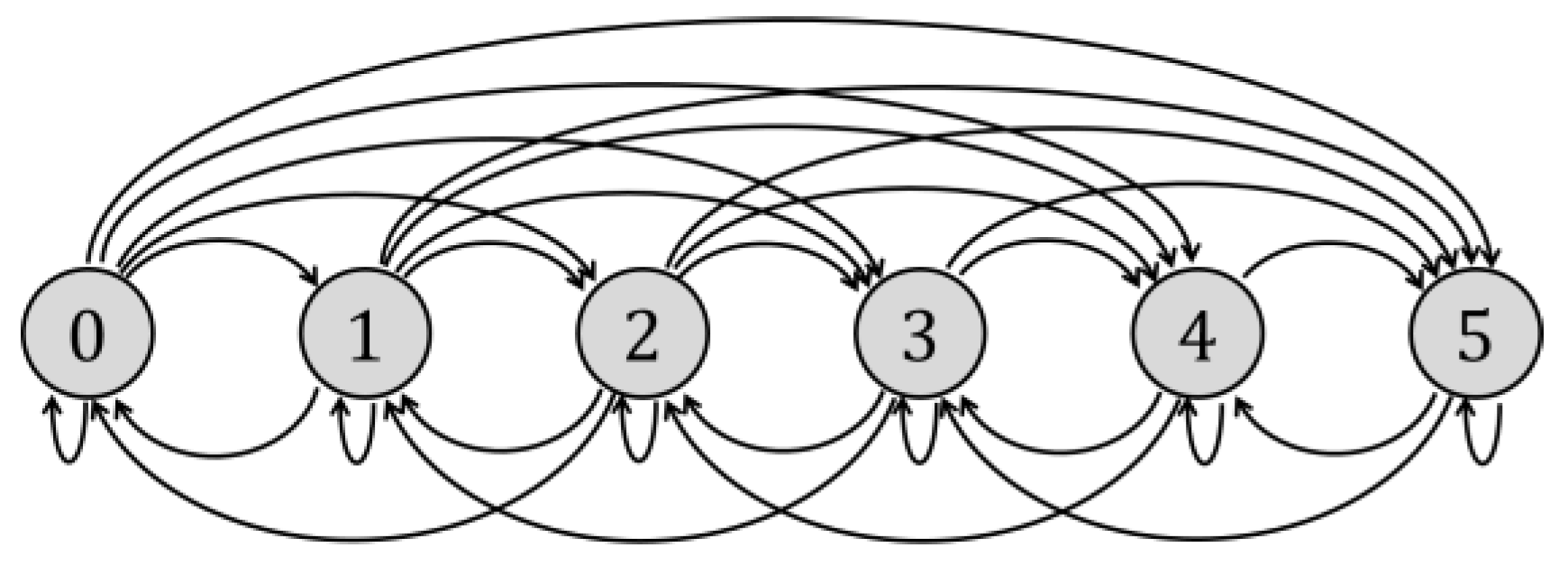
3.3. Two or More Machines in Operation

The difference between this case and the case of a single machine in operation is that we now have the possibility that two machines can suffer damage in a single day. For example, let us consider the case where there are two machines operating, each one with a critical component, and three spare critical components. By considering the daily transition possibilities of the states that reflect these components, we arrive at Figure 2.

In Figure 2, the possibility that all faulty components can be repaired at the same time is considered. This is why there is a possibility that state 5 can be reached from state 0 in a single step. Additionally, since it is possible for two machines to be in operation on a single day, and both components could experience failures, if neither machine is repaired, state 0 can be reached directly from state 2 in a single step.

Let R be the probability that a component that failed today will be in good condition tomorrow, and let F be the probability that a component that is in good condition today will fail tomorrow. Then, the transition probabilities of the Markov chain can be obtained using the equations in

Table 5. Description for the calculation of the probabilities of transition between the different states for the case of two operating machines.

State	0	1	2	3	4	5
0	[1 − R]5	5[1 − R]4 R	10[1 − R]3 R2	10[1 − R]2 R3	5[1 − R] R4	R5
1	[1 − R]4 F	[1 − R]4 [1 − F] + 4 [1 − R]3 RF	4 [1 − R]3 R [1 − F] + 6 [1 − R]2 R2 F	6[1 − R]2 R2 [1 − F] + 4[1 − R] R3 F	4[1 − R] R3 [1 − F] + R4 F	R4 [1 − F]
2	[1 − R]3 F2	2 [1 − R]3 F [1 − F] + 3[1 − R]2 R F2	3[1 − R] R2 F2 + 6[1 − R]2 RF [1 − F] + [1 − R]3 [1 − F]2	R3 F2 + 6[1 − R] R2 F [1 − F] + 3[1 − R]2 R [1 − F]2	2 R3 F [1 − F] + 3[1 − R] R2 [1 − F]2	R3 [1 − F]2
3	0	[1 − R]2 F2	2 [1 − R]2 F [1 − F] + 2[1 − R] R F2	R2 F2 + 4[1 − R] R F [1 − F] + [1 − R]2 [1 − F]2	2 R2 [1 − F] F + 2[1 − R] R [1 − F]2	R2 [1 − F]2
4	0	0	[1 − R] F2	2 [1 − R] F [1 − F] + R F2	[1 − R] [1 − F]2 + 2 R F [1 − F]	R [1 − F]2
5	0	0	0	F2	2 F [1 − F]	[1 − F]2

.

The process of constructing Table 5 closely resembles that of Table 1. However, in this case, we must consider the probabilities of more than one machine failing in the next iteration. For instance, if the system is in state 2 and we want to calculate the probability that the system will be in state 3 in the next iteration, we need to consider the following possibilities:

(1)

Neither of the two operating machines fails and is shut down, and one of the other three machines is repaired.

(2)

One of the operating machines fails, but two of the machines under repair are restored.

(3)

Both operating machines fail, but the three machines that were in the repair process are restored.

Each of these scenarios has a corresponding probability associated with it, and by summing up these probabilities, we can determine the overall probability of transitioning from state 2 to state 3. Similarly, for other states and transitions, we need to consider all the possible combinations of machine failures and repairs to obtain the transition probabilities accurately.

For example, suppose the failure rate of a certain component is once every 200 days and the average time that component spends on the shop floor until it is repaired is 20 days. Then R = 0.04877, while F = 0.00499

The matrix that represents the transition probabilities is given in

Table 6. Transition probabilities for the problem of two machines in operation with three spare parts.

State	0	1	2	3	4	5
0	0.77880	0.19965	0.02047	0.00105	0.00003	0.00000
1	0.00408	0.81548	0.16714	0.01285	0.00044	0.00001
2	0.00002	0.00855	0.85346	0.13114	0.00672	0.00011
3	0.00000	0.00002	0.00898	0.89676	0.09188	0.00235
4	0.00000	0.00000	0.00002	0.00944	0.94225	0.04829
5	0.00000	0.00000	0.00000	0.00002	0.00993	0.99005

.

Table 7. Steady-state probabilities for the case of two machines.

State	0	1	2	3	4	5
Markov Chain	0.00000	0.00006	0.00113	0.01691	0.16708	0.81482
Simulation	0.00001	0.00003	0.00101	0.01586	0.16195	0.82112

presents the results of a simulation performed in the ARENA software for one million days.

As can be seen, the results of the simulation and those obtained through the transition matrix are similar.

Again, 50 chi-square tests were performed to determine the possibility of significant differences between the two methods. We experimented with different numbers of components in use, different numbers of spare parts, and different failure and repair rates. In no case is it possible to determine significant differences. The results under both methods are extremely similar, and the differences between the two methods in 99% of cases differ by less than one-hundredth.

Moreover, we also performed tests to determine if the steady-state probabilities remain constant when the ratio of the repair rate to the failure rate is equivalent. That is, in the example above, we observed that the time to repair is 20 days, while the time between failures is 200 days, so the ratio = 20/200 = 0.1. The assumption is that the results for a failure ratio that is equivalent to 0.1 should be very similar.

As in the case of a single machine, when the ratios r are alike, the steady-state probabilities are very similar.

3.4. The Case of Machines with Exponential Failure Time and Other Distributions of Repair Times

A fundamental factor to consider when modeling a process using Markov chains is that the evolution of the process in the future depends only on the present state and does not depend on the history; this property is called “memoryless”, and it is not a common property in the probability distributions. In fact, the memoryless property occurs in only two distributions: the geometric distribution and the exponential distribution [37]. This is the fundamental reason for assuming that both repair times and failure times are exponentially distributed.

Moreover, the assumption that component failure times are exponentially distributed is not a strange or unrealistic assumption; see, for example, [38,39]. On the other hand, repair times are also modeled according to the exponential and other types of distributions [39,40]. In this research, some simulation tests were run assuming that the repair times are constant, normal, uniform, and triangular. It is important to remark that the steady-state results obtained by the theoretical transition matrices are very similar to the results obtained by the simulation, considering that 0 < r ≤ <= 0.4. It is also important to note that the lower the value of the ratio r, the more similar the results obtained through the simulation and those obtained from the steady-state values are.

As an example,

Table 8. Steady-state probabilities with r = 0.4 and different failure rates for the case of two operating machines.

State	0	1	2	3	4	5	6	7
Markov Chain	0.29958	0.36175	0.21796	0.08736	0.02621	0.00626	0.00084	0.00005
Sim N (80, 2)	0.30306	0.36535	0.20817	0.08660	0.02880	0.00693	0.00109	0.00000
Sim N (80, 10)	0.30412	0.36478	0.20608	0.08761	0.02927	0.00718	0.00093	0.00003
Sim N (80, 20)	0.30550	0.36335	0.20412	0.09016	0.02880	0.00725	0.00079	0.00004
Sim N (80, 40)	0.30224	0.36227	0.20793	0.09110	0.02847	0.00723	0.00067	0.00009

shows that the results obtained by the simulation and the results obtained by the Markov chain are very similar. In this case, it is assumed that the failure times are distributed exponentially, with λ_F = 1/200, and the repair times are normally distributed with a mean of 80 days. We carried out the simulations considering different variances and ran the simulations for one million days.

In Table 8, the first row describes the steady-state probabilities considering two operating machines and five spare machines. The other lines describe the simulation results considering normal distributions with mean 80 and different standard deviations. As can be seen in the table, the results obtained in the case of the normal distribution differ from the results obtained by modeling the Markov chain by less than eleven-thousandths.

Furthermore, when the results of the steady-state probabilities are compared to other repair times that follow a uniform or triangular distribution, or these repair times are constant, the differences between the simulations and the Markov chain modeling are even smaller. The only condition requested is that the average repair times must generate the same ratio r that is being used in the Markov chain.

Overall, the simulation results closely align with the Markov chain modeling results, indicating the reliability and accuracy of the proposed approach in analyzing the system’s behavior under various repair time distributions. The close correspondence between the results validates the suitability of the Markov chain model for spare parts management, even when considering different repair time probability distributions.

We performed 100 chi-square tests to determine the possibility of significant differences between the two methods. We experimented with different distributions, different numbers of components in use, different numbers of spare parts, different times between failures, and different times to repair. Similarly to the case of the exponential distribution, in none of the cases was it possible to determine significant differences.

Based on the results that have been obtained in this section, it can be argued that the results can be extended to constant repair times, and repair times with normal, uniform and triangular distributions. These findings are similar to those obtained in [37], where it is stated that “simple Markov models with exponential repair-time densities can be used and will give the same results as more complicated non-exponential repair-time densities”.

3.5. The Case of a Single Machine with Weibull Distribution Failure Time and Other Distributions of Repair Times

One of the most widely accepted distributions of failure times is the Weibull distribution [41,42]. When we use the Weibull distribution for the time between failures in the simulation, the steady-state probabilities obtained by the Markov chain differ from the results obtained by the simulation when 0.1 < r, that is, the results are only reliable if 0 < r ≤ 0.1. Although the results seem quite limited, if we consider a component with an average failure time of one year, a corresponding repair time of 36 days or less is quite adequate.

4. Cost Analysis and Construction of Solution Frontiers

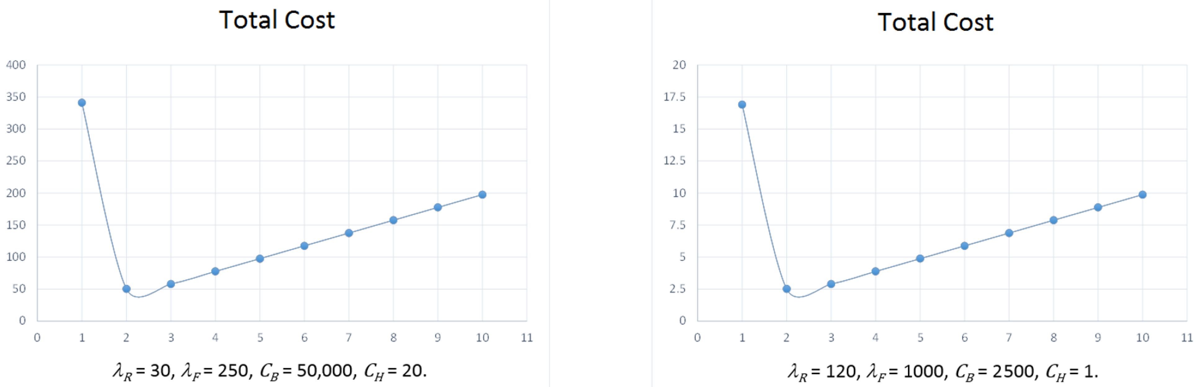
4.1. Analyzing the Costs of the Model for the Case of a Single Machine

Obtaining steady-state probabilities is critical to obtaining the total costs of a policy. For example, suppose we have a company that operates a machine. This machine has a component whose value is $10,000. If the machine stops working one day, the company has a loss of $400,000. On the other hand, if a component fails, it is sent to a workshop and the daily cost of repair is $100 per day. The annual cost of keeping a component in inventory is 30% of the value of the component. The failure rate of this component is once every 250 days, and the average repair time is 25 days. Finally, suppose a year has 300 business days.

Notation:

C_H = Maintenance cost per unit per day

C_B = Daily cost when the machine is idle

C_R = Daily repair cost

P_i = The steady-state probability of state i

The relevant information for the scenario described above is as follows:

C_H = 0.30 (10,000)/300 = $10/day, C_B = $400,000/day, and C_R = $100/day.

In this case, we can obtain the costs of a policy of having two spare components as follows (we approximate the results to the rate in Table 2 that most closely resembles the coefficients of the problem, that is, we take the steady-state probabilities of a 200-day time between failures and a 20-day time to repair).

Note that when the system is in state 3, there will be two units in inventory; when the system is in state 2, there will be one unit in inventory; and when the system is in state 1 or state 0, there will be no units in inventory. Therefore, the maintenance cost per day can be approximated as $10 (P₂ + 2P₃) = $18.98/day.

On the other hand, the cost of not having an available, operational component (backorder) occurs only when the system is in state 0, so the daily cost for a backorder is determined by the number $400,000 P₀ = $60.00/day.

Finally, note that if the system is in states 3, 2, 1, or 0, there will be 0, 1, 2, or 3 units being repaired, respectively. The daily cost of repairs will be $100 (3P₀ + 2P₁ + P₂) = $10.21.

Therefore, the total cost of the policy of having two replacement parts is the sum of $18.98, $60.00, and $10.21, that is, $89.19/day.

Let us consider the possibility of analyzing the behavior of the cost function with these parameters (C_H = 10, C_B = 400,000, C_R = 100). To do this, we will follow a specific methodology where we keep two of these costs fixed and then study how the values of one of them modify the shape of the graph.

In other words, we will hold two of the costs (say C_H and C_B) constant while varying the value of the third cost (in this case, C_R). By doing so, we can observe how changes in the value of the third cost influence the total cost function and its graphical representation.

This approach allows us to investigate the individual impact of each cost parameter on the total cost function and gain insights into how they interact with one another to determine the overall cost structure. Through this sensitivity analysis, it is possible to gain valuable insights into which parameters have the most significant impact on the cost function and, consequently, on the optimal solution to the problem. This understanding will help with making informed decisions and fine-tuning the parameters to optimize the cost and achieve the best possible solution for the given scenario.

Figure 3 shows the total cost as a function of C_H, C_B, and C_R. The horizontal axis is the number of spare parts considered, and the vertical axis is the total cost of the policy. The values of C_H and C_B are kept constant, while the graph shows the behavior of the costs for the different values of C_R.

The values of C_R vary from 0 to 1000. The variation in different C_R values is reflected through vertical axis translations, but the shape of the curve remains unchanged. As a result, the optimal value for the number of spare parts remains constant at three, regardless of the C_R value. This important conclusion indicates that the value of the C_R parameter does not affect the optimal number of spare parts. This finding is significant because it demonstrates that the C_R value does not impact the decision regarding the number of spare parts required.

In Figure 4, C_H and C_R are constants. The graph shows the behavior of the total cost for different values of C_B in a range of 50,000 to 1,000,000. Note that for small values of C_B, the optimal number of spare parts could be two units, while for values of 100,000 onwards, the optimal number of spare parts is three units. In this case, it is possible to affirm that the value of C_B modifies the behavior of the graph.

In Figure 5, the values of C_B and C_R are held constant, while the graphs illustrate the cost behavior for various values of C_H (ranging from 2 to 80). Notably, the shape of the curves in Figure 5 differs from those in Figure 3 and Figure 4. Specifically, when C_H is set to 2, the optimal solution is to store three spare components. In contrast, when C_H is set to 80, the optimal solution is to keep two spare components. This observation highlights the sensitivity of the optimal solution to changes in the value of C_H. As C_H increases, the optimal number of spare components decreases. Conversely, as C_H decreases, the optimal number of spare components increases.

As can be seen, although C_B, C_H, and C_R produce alterations in the total cost curves, the value of C_R only seems to cause a translation of the curve on the vertical axis, which does not affect the optimal number of spare machines. For this reason, we can consider that the objective function depends on four variables, namely λ_R, λ_F, C_B, and C_H, and use another graphical approach to simplify the analysis by integrating the four variables into two, r and c = C_B/C_H.

Suppose we have a scenario where 1/λ_R = 30, 1/λ_F = 250, C_B = $50,000, and C_H = $20. This scenario should be equivalent to a problem where 1/λ_R = 120, 1/λ_F = 1000, C_B = $2500, and C_H = $1, since in both cases, r = 0.12 and c = 2500. Figure 6 shows the corresponding graphs for the two cases. In both figures, the vertical axis represents the total cost function and the horizontal axis corresponds to the number of replacement units. Despite the higher costs being evident in the figure on the left, what we want to emphasize is that both figures exhibit the same shape, and the optimal solution in both cases is to have two spare components. In other words, the problems solved are equivalent, although the values of the costs and times differ between the problems.

Using this characteristic, the optimal number of spare parts can be obtained considering only two variables, c and r.

As can be assumed, if the values of r and c are small (that is, if the repair time is very small with respect to the failure rate and the cost of a missing part is small in relation to the cost of having a part in inventory), the number of spare parts should also be small.

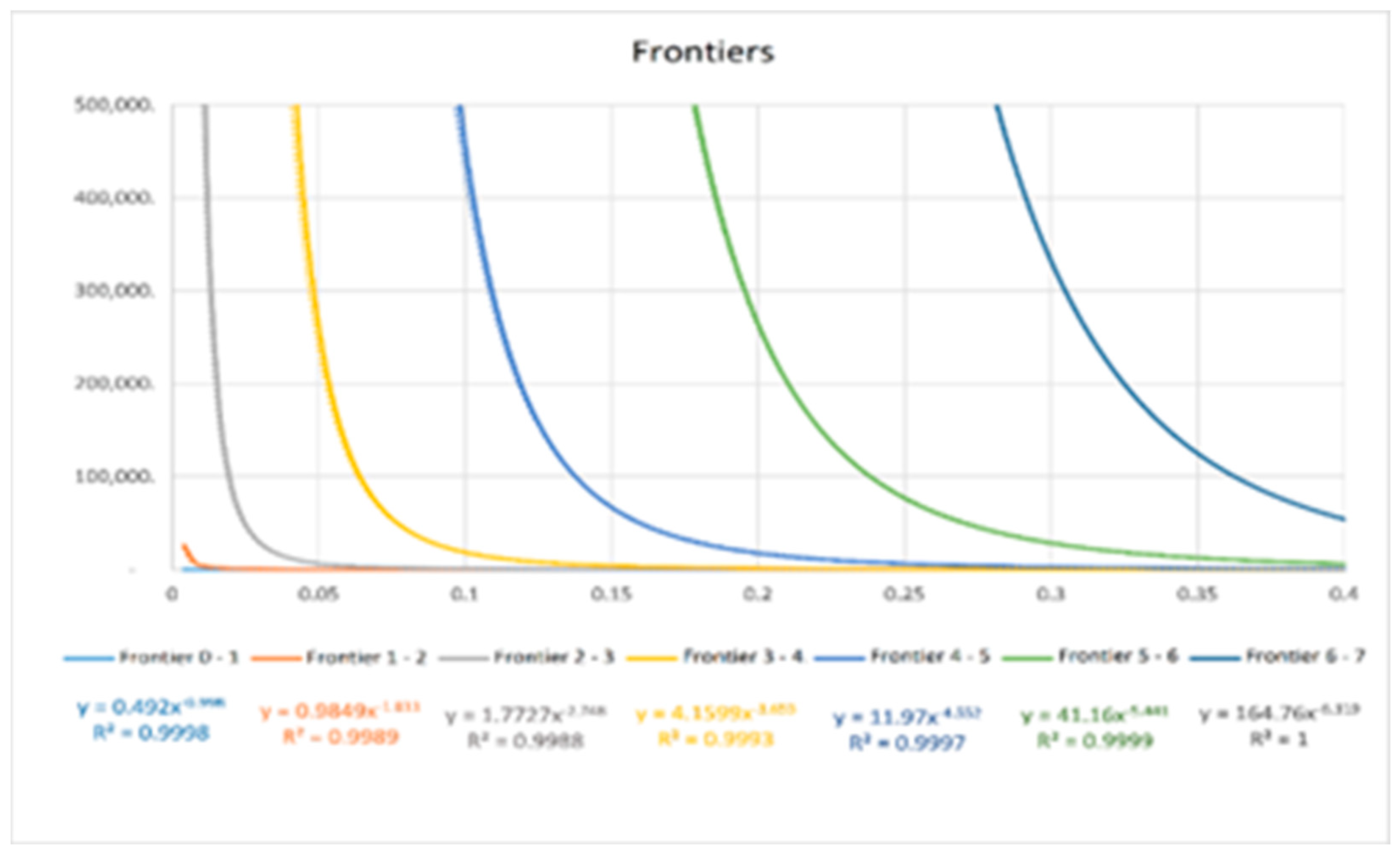
4.2. Building the Model Solution

In the case of a single machine, we constructed a graph (Figure 7) to easily find the optimal number of spare parts for a given pair of values c and r. Figure 7 is constructed considering that r can vary on the horizontal axis in the interval (0, 0.4] and the variable c can vary on the vertical axis in the interval (0, 10,000).

In the blue section, the optimal number of spare parts is 0; in the orange section, the optimal number of spare parts is 1; in the gray section, the optimal number of spare parts is 2; and in the yellow section, the optimal number of spare parts is 3.

Based on this diagram, we found the values of c and r where the costs of having 0 spare parts and 1 spare part were the same. Then, we found the values of c and r where the costs of having 1 and 2 spare parts were the same, and so on. The range of r values we considered is (0, 0.4), while the values of c vary in the range (0, 1,000,000]. Once the points were obtained, a regression was performed to obtain fitted equations for these curves. The results are shown in Figure 8. The horizontal axis represents the values of r, while the vertical axis represents the values of c.

As can be seen, the R² values obtained from these equations are very close to 1. Therefore, we conclude that the equations can be used for decision making with almost no risk.

For the selected intervals of c and r, the frontiers are defined by the curves:

• Frontier 0–1: c = 1.2018 r^−0.944
• Frontier 1–2: c = 3.3336 r^−1.857
• Frontier 2–3: c = 10.563 r^−2.829
• Frontier 3–4: c = 45.833 r^−3.769
• Frontier 4–5: c = 251.33 r^−4.692
• Frontier 5–6: c = 1656.0 r^−5.603

Once these equations have been obtained, the Algorithm 1 is developed for obtaining the optimal number of spare parts is the following:

Algorithm 1 Finding the optimal number of spare parts

Step 1. Compute c0 = CB/CH and $r=\frac{\frac{1}{{\lambda }_R}}{\frac{1}{{\lambda }_F}}$

Step 2. Set i = 1

Step 3. Using r, evaluate c using frontier equation i.

Step 4. If c > c0, proceed to step 5. Otherwise, set i = i + 1 and go back to step 3.

Step 5. Obtain the optimal value of spare parts.

Consider again the example where λR = 1/30, λF = 1/250 CH = 20 and CB = 50,000. Now,

Step 1. c0 = CB/CH = 2500 y r = = 0.120

Step 2. i = 1

Step 3. F (0–1): c = 1.2018 (0.120)–0.944 = 8.89

Step 4. 8.89 < 2500; i = 2

Step 3. F (1–2): c = 3. 3336 (0.120)–1.857 = 170.95

Step 4. 170.95 < 2500; i = 3

Step 3. F (2–3): c = 10.563 (0.120)–2.829 = 4253.86

Step 4. 4253.86 > 2500

Step 5. The optimal number of spare parts is 2, the lower limit of the interval (2–3).

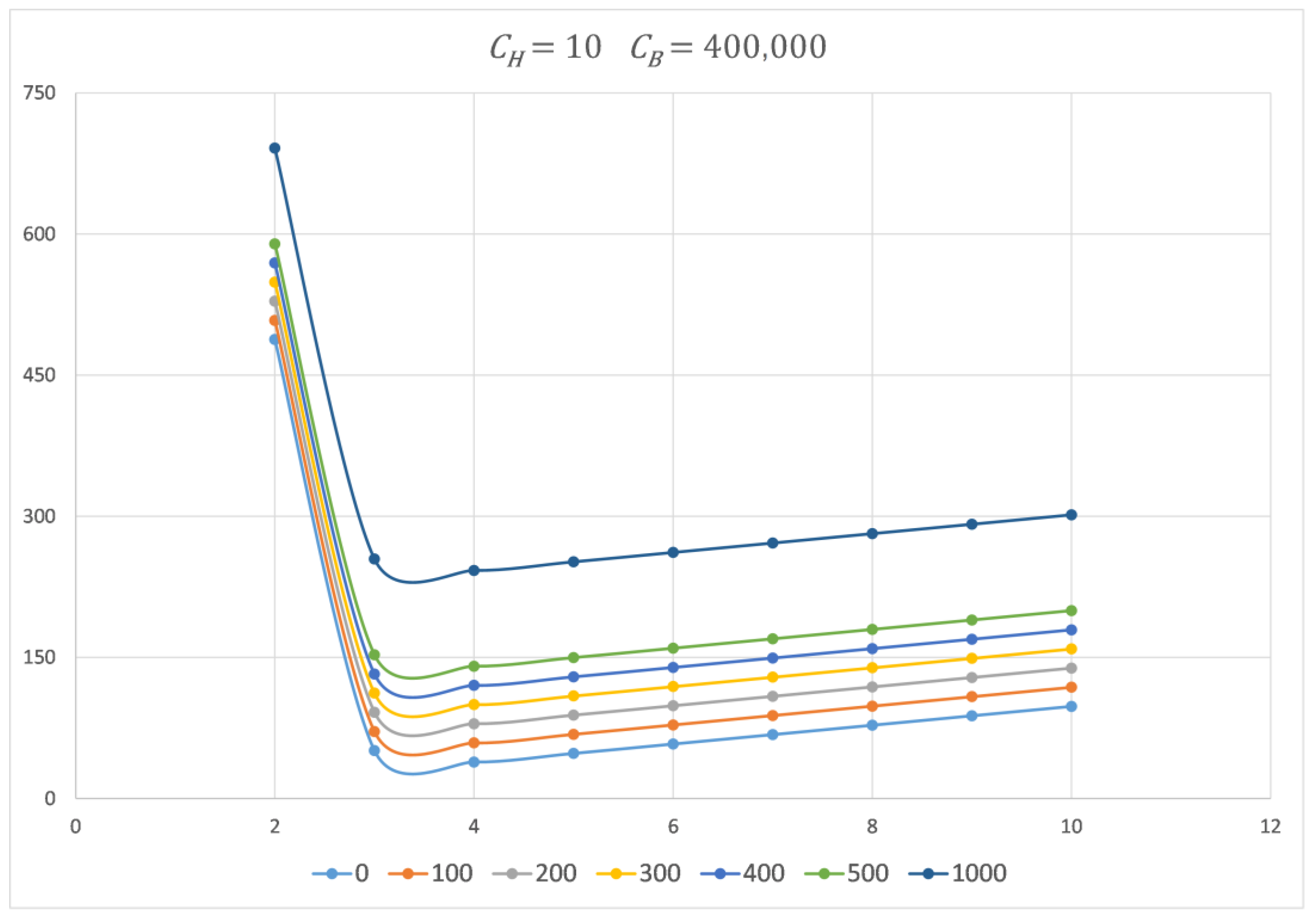
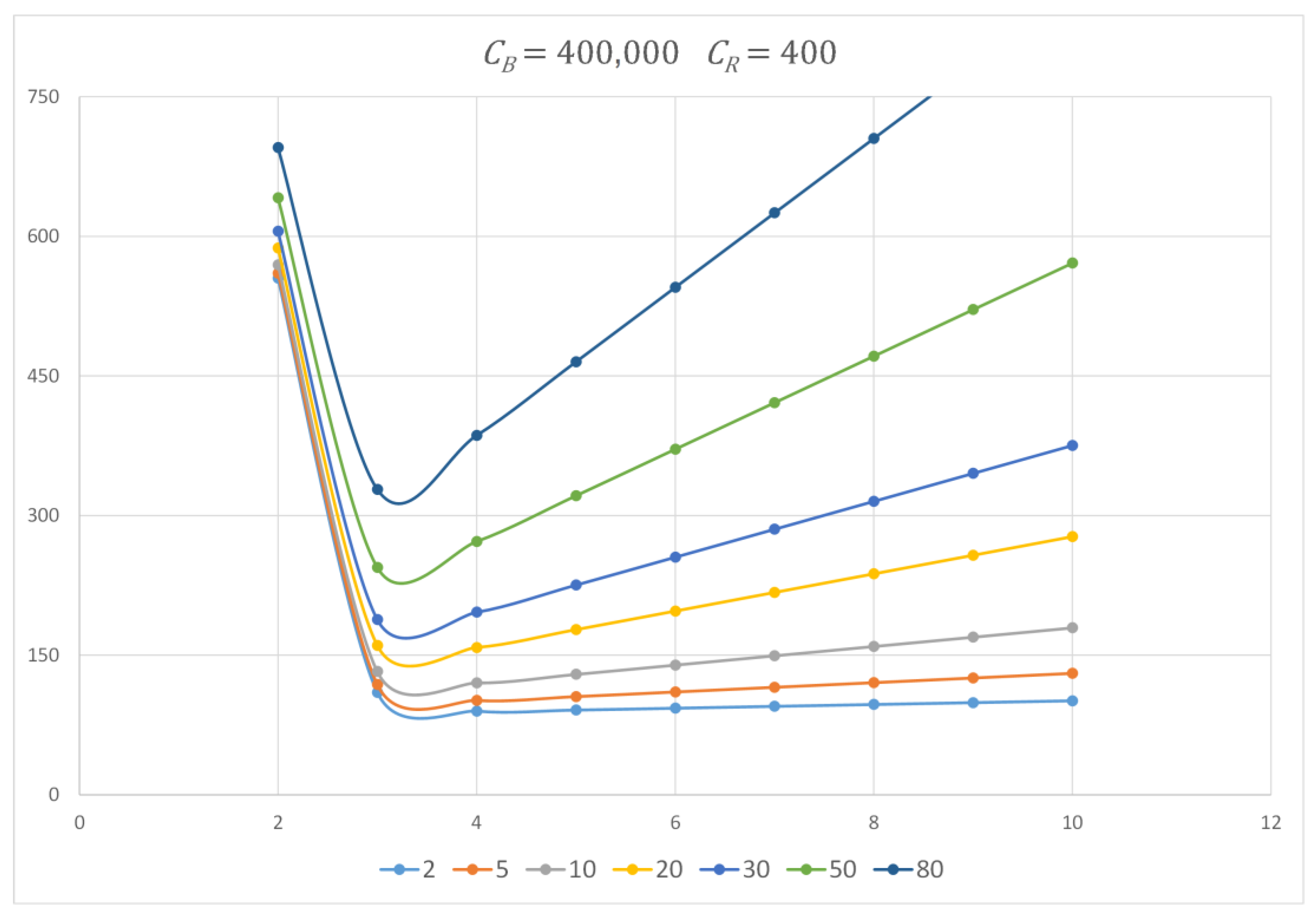
4.3. Analyzing the Costs of the Model for the Case of n Machines

Let us now consider the calculation of costs in the case of two machines running and considering three spare machines. For example, suppose we have a company that operates with two machines and these machines have a component whose value is $10,000. If one machine stops working one day, the company has a loss of $400,000. When a component fails, it is sent to a workshop and the daily cost of repair is $100 per day. The annual cost of keeping a component in inventory is 30% of the value of the component. The failure rate of this component is once every 250 days, and the average repair time is 25 days. Finally, suppose a year has 300 business days. Transforming this problem to daily costs yields the following values:

C_H = Maintenance cost per unit per day = 0.30 (10,000)/300 = $10/day

C_B = $400,000/day

C_R = $100/day

In this case, we can obtain the costs of a policy of keeping two spare components as follows (we will approximate the results to the rate in Table 6 that most closely resembles the coefficients of the problem, that is, in this case, we take the steady-state probabilities of a 200-day failure time rate and a 20-day repair rate).

Note that when the system is in state 3, there will be one unit in inventory; when the system is in state 4, there will be two units in inventory; when the system is in state 5, there will be three units in inventory; and if the system is in state 2, state 1, or state 0, there will be no units in inventory. Therefore, the maintenance cost per day is $10 (P₃ + 2P₄ + 3P₅) = $27.96.

When the system is in state 1, there is one stockout, and when the system is in state 0, there are two stockouts. Therefore, the expected backorder cost is $400,000 (P₁ + 2P₀) = $23.03.

Finally, if the system is in state 5, state 4, or state 3, there will be no units, one unit, and two units being repaired, respectively. Then, the daily cost of repairs can be calculated as $100 (5P₀ + 4P₁ + 3P₂ + 2P₃ + P₄) = $20.36.

By adding the three costs shown above, we determine that the total daily cost of this policy will be $71.36.

Just like in the case of a single machine, we will analyze how each of the different costs affects the total cost graph. By examining the impact of individual cost parameters, we can gain a comprehensive understanding of their influence on the overall cost function and optimize the decision-making process for spare parts management.

In Figure 9, the horizontal axis is the number of spare parts, and the vertical axis is the cost of the policy. It has been decided to leave as constant the values of C_H and C_B, while the graph shows the behavior of the costs for different values of C_R.

In this graph, we have taken the values corresponding to this example, and we have varied the value of C_R in the range from 0 to 1000. Note that the shape of the curve is not altered by the different values of C_R and therefore, in all cases, the optimal value for the number of spare parts is four machines. The value of C_R only causes a translation of the curve on the vertical axis, which does not affect the optimal number of spare machines. Despite the different values of C_R, the shape of the curve remains the same, and the optimal number of spare machines consistently remains four.

In Figure 10, the values of C_H and C_R are fixed, while the graph shows the behavior of the costs for different values of C_B. Note that the shapes of Figure 10 are different from the shapes in Figure 9 and that even in the first two cases (C_B = 50,000, C_B = 100,000), the optimal solution is to have three spare parts, whereas if C_B ≥ 200,000, the optimal solution is to have four spare parts.

Finally, in Figure 11, the values of C_B and C_R are fixed. The graph shows the behavior of the costs for the different values of C_H. Note that now the curves’ shapes in Figure 11 are again modified compared to Figure 9 and Figure 10. In the first cases (C_H = 2, C_H = 5, C_H = 10), the optimal solution is to have four spare parts, while in the last cases (C_H >= 20), the optimal solution is to have three spare parts.

It can be observed that, although the three costs produce alterations in the total cost curves, the value of C_R only seems to have a translation effect on the curves on the vertical axis, which does not affect the optimal number of spare components.

As in the case of a single machine, a graph is constructed to find the optimal number of spare parts. The idea is the same as before: to find the values of c and r where the costs of having 0 spare parts and 1 spare part would be the same. Then, those points having 1 and 2 spare parts were the same, and so on. The range of r values is considered in the range (0, 0.4), while the values of c vary in the range (0, 1,000,000]. Once the points were obtained, a regression was performed to obtain the fitted equation of these points. The results are shown in Figure 12. As in Figure 7, the dotted curves represent the fitted equations, and the solid curves represent the observed values.

As can be seen, the R² values obtained from these equations are very close to 1. Therefore, equations can be used for decision making.

The graphs and the corresponding fitted equations can be easily found for any number of machines. When the equations are obtained, the procedure for determining the optimal number of spare parts is the same as in the case of a single machine.

Since R² > 0.99 in all fitted equations, the number of spare parts suggested by this method should be the optimal solution in more than 99% of cases, and in the few cases where a difference from the optimal number of spare parts is found, the difference between the two costs is very small.

Even though the graphs are limited in the intervals 0 < r < 0.4 and 0 < c < 500,000, the regression equations are calculated in the ranges 0 < r < 0. 5 and 0 < c < 1,000,000.

The frontier equations for the cases from one to five machines are shown in

Table 9. Frontier equations.

	Number of Machines
Frontier	1	2	3	4	5
Frontier 0–1	c = 1.2018 r−0.944	c = 0.4920 r−0.998	c = 0.2752 r−1.043	c = 0.1611 r−1.113	c = 0.1075 r−1.160
Frontier 1–2	c = 3.3336 r−1.857	c = 0.9849 r−1.811	c = 0.5134 r−1.769	c = 0.2879 r−1.779	c = 0.1995 r−1.761
Frontier 2–3	c = 10.563 r−2.829	c = 1.7727 r−2.748	c = 0.7375 r−2.658	c = 0.3524 r−2. 633	c = 0.2370 r−2.558
Frontier 3–4	c = 45.833 r−1.769	c = 4.1599 r−1.653	c = 1.3626 r−3.497	c = 0.4766 r−3. 501	c = 0.2931 r−3.385
Frontier 4–5	c = 251.33 r−4.692	c = 11.97 r−4.552	c = 3.1677 r−4.297	c = 0.7549 r−4.366	c = 0.4377 r−4.177
Frontier 5–6	c = 1656 r−5.603	c = 41.16 r−5.441	c = 9.0753 r−5.056	c = 1.3954 r−5.227	c = 0.7683 r−4.950
Frontier 6–7		c = 164.76 r−6.319	c = 34.984 r−5.681	c = 2.9798 r−6.080	c = 1.6729 r−5.655
Frontier 7–8			c = 171.99 r−6.180	c = 7.1632 r−6.932	c = 4.3101 r−6.311
Frontier 8–9				c = 19.384 r−7.771	c = 4.1265 r−7.626
Frontier 9–10				c = 57.260 r−8.614	c = 10.068 r−8.451

. These equations can be used to plot the curves, which will allow decision-makers to easily find the optimal solution.

The graph of the boundary equations indeed proves to be a valuable tool in obtaining the solution easily. For instance, consider the case of two machines with r = 0.10 and c = 100,000. If we plot the point (0.10, 100,000) on Figure 12, we can observe that this point lies between the Frontier 3–4 (yellow line) and the Frontier 4–5 (blue line). Therefore, the optimal number of spare machines should be four. In fact, the expected value of total cost with three spare units is $104.91, the expected value of total cost with five spare units is $68.12, and the expected value of total cost with four spare units is $60.30.

In addition, all those cases in which the points are between the yellow line and the blue line have as a solution that the optimal number of spare parts will be four. This has the consequence that in the vast majority of cases, the solution can be obtained visually from the figure, and it is only necessary to execute the algorithm when the point to be evaluated is very close to one of the borderlines. The graph provides an intuitive representation of the optimal inventory strategy based on the given cost parameters.

This visual approach is highly advantageous, as it allows for quick and efficient decision making. However, in cases where points are located near the frontier lines, executing the algorithm becomes essential to precisely determine the optimal number of spare machines. By combining both visual analysis and algorithmic evaluation, the boundary equations graph becomes a powerful tool for spare parts inventory management, facilitating accurate decision making and minimizing computational efforts.

5. Conclusions and Future Research

5.1. Conclusions

This document presents a study focused on modeling a spare parts inventory system using the Markov chain approach. To assess the accuracy of this modeling, various simulations were conducted, and the steady-state results of the system were validated. The simulations and Markov chains show significant similarities, confirming the tool’s effectiveness in representing the spare parts inventory system.

The study considers three costs in the system: the cost of holding a spare part in inventory (CH), the cost of a missing part (CB), and the cost of repairing parts in the workshop (CR). The analysis indicates that CR impacts the cost behavior, leading to a translation of the vertical axis in the graph. However, it does not alter the graph’s shape or behavior, suggesting that the repair cost is not critical in determining the optimal number of spare parts.

The study highlights the analysis of four crucial variables that require consideration: the failure rate of parts in the system, the repair rate of parts in the workshop, the cost of maintaining a part in inventory, and the cost of a missing part. These variables significantly influence the performance and profitability of the spare parts inventory system.

By incorporating these variables into the system model, it becomes possible to establish boundaries where the policy of having n spare parts is equivalent to the policy of (n + 1) spare parts. The cost curves corresponding to these boundaries can be effectively modeled using exponential functions. Leveraging these models, one can easily determine the optimal policy for an inventory system across various values of the variables examined in the study.

The ability to plot cost curves with exponential functions simplifies the decision-making process, enabling quick and accurate identification of the most profitable inventory strategy. By thoroughly analyzing the impact of each variable on the cost function, organizations can make informed decisions to minimize costs and ensure optimal spare parts management.

5.2. Limitations and Future Research

The model’s scope is limited to spare parts that can be repaired and assumes the possibility of multiple spare parts being repaired simultaneously.

It is convenient for analyzing the operation of a chain in the case of business models where spare parts are requested by external customers, and these parts become lost sales, or they can be supplied through backorders.

It would also be desirable to use the methodology to consider different costs, such as economic penalties or the obsolescence of some parts.

References

1. Muckstadt, J.A.; Sapra, A. Principles of Inventory Management: When You Are Down to Four, Order More. In Springer Series in Operations Research and Financial Engineering; Springer: New York, NY, USA, 2010. [Google Scholar] [CrossRef]
2. Shah, N.H.; Mittal, M.; Cárdenas-Barrón, L.E. (Eds.) Decision Making in Inventory Management. In Inventory Optimization; Springer: Singapore, 2021. [Google Scholar] [CrossRef]
3. Kennedy, W.; Patterson, J.W.; Fredendall, L.D. An overview of recent literature on spare parts inventories. Int. J. Prod. Econ. 2002, 76, 201–215. [Google Scholar] [CrossRef]
4. Botter, R.; Fortuin, L. Stocking strategy for service parts—A case study. Int. J. Oper. Prod. Manag. 2000, 20, 656–674. [Google Scholar] [CrossRef]
5. Hu, Q.; Bai, Y.; Zhao, J.; Cao, W. Modeling Spare Parts Demands Forecast under Two-Dimensional Preventive Maintenance Policy. Math. Probl. Eng. 2015, 2015, 728241. [Google Scholar] [CrossRef]
6. Muniz, L.R.; Conceição, S.V.; Rodrigues, L.F.; Almeida, J.F.d.F.; Affonso, T.B. Spare parts inventory management: A new hybrid approach. Int. J. Logist. Manag. 2021, 32, 40–67. [Google Scholar] [CrossRef]
7. Al-Kaabi, H.; Potter, A.T.; Naim, M.M. Insights into the Maintenance, Repair, and Overhaul Configurations of European Airlines. J. Air Transp. 2007, 12, 2. [Google Scholar]
8. Eriksson, S.; Steenhuis, H.-J. The Global Commercial Aviation Industry; Routledge: Oxfordshire, UK, 2015. [Google Scholar]
9. Wang, L.; Chu, J.; Mao, W. A condition-based order-replacement policy for a single-unit system. Appl. Math. Model. 2008, 32, 2274–2289. [Google Scholar] [CrossRef]
10. Do Rego, J.R. A Lacuna Entre a Teoria de Gestão de Estoques e a Prática Empresarial na Reposição de Peças em Concessionárias de Automóveis. Ph.D. Thesis, Universidade de São Paulo, São Paulo, Brasil, 2006. [Google Scholar]
11. Kumar, S. Parts Management Models and Applications: A Supply Chain System Integration Perspective; Springer: New York, NY, USA, 2005. [Google Scholar]
12. Muckstadt, J.A. Analysis and Algorithms for Service Parts Supply Chains; Springer Science & Business Media: Berlin/Heidelberg, Germany, 2006. [Google Scholar]
13. Rego, J.R.D.; de Mesquita, M.A. Controle de estoque de peças de reposição em local único: Uma revisão da literatura. Production 2011, 21, 645–666. [Google Scholar] [CrossRef]
14. Gomes, A.V.P.; Wanke, P. Modelagem da gestão de estoques de peças de reposição através de cadeias de Markov. Gest. Prod. 2008, 15, 57–72. [Google Scholar] [CrossRef]
15. Strijbosch, L.; Moors, J. Modified normal demand distributions in (R,S)-inventory control. Eur. J. Oper. Res. 2006, 172, 201–212. [Google Scholar] [CrossRef]
16. Thomopoulos, N.T. Demand Forecasting for Inventory Control. In Demand Forecasting for Inventory Control; Springer International Publishing: Cham, Switzerland, 2015; pp. 1–10. [Google Scholar] [CrossRef]
17. Bain, L.J.; Engelhardt, M. Statistical Analysis of Reliability and Life-Testing Models: Theory and Methods, 2nd ed.; Routledge: Oxfordshire, UK, 2017. [Google Scholar] [CrossRef]
18. Engelhardt, M. Reliability Estimation and Applications. In The Exponential Distribution, 1st ed.; Balakrishnan, N., Basu, A.P., Eds.; Routledge: Oxfordshire, UK, 2019; pp. 73–91. [Google Scholar] [CrossRef]
19. Braglia, M.; Grassi, A.; Montanari, R. Multi-attribute classification method for spare parts inventory management. J. Qual. Maint. Eng. 2004, 10, 55–65. [Google Scholar] [CrossRef]
20. Lolli, F.; Balugani, E.; Ishizaka, A.; Gamberini, R.; Rimini, B.; Regattieri, A. Machine learning for multi-criteria inventory classification applied to intermittent demand. Prod. Plan. Control 2018, 30, 76–89. [Google Scholar] [CrossRef]
21. Syntetos, A.A.; Boylan, J.E.; Croston, J.D. On the categorization of demand patterns. J. Oper. Res. Soc. 2005, 56, 495–503. [Google Scholar] [CrossRef]
22. Boylan, J.E.; Syntetos, A.A.; Karakostas, G.C. Classification for forecasting and stock control: A case study. J. Oper. Res. Soc. 2008, 59, 473–481. [Google Scholar] [CrossRef]
23. Ilgin, M.A.; Tunali, S. Joint optimization of spare parts inventory and maintenance policies using genetic algorithms. Int. J. Adv. Manuf. Technol. 2007, 34, 594–604. [Google Scholar] [CrossRef]
24. Díaz, A.; Fu, M.C. Models for multi-echelon repairable item inventory systems with limited repair capacity. Eur. J. Oper. Res. 1997, 97, 480–492. [Google Scholar] [CrossRef]
25. Brick, E.S.; Uchoa, E. A facility location and installation of resources model for level of repair analysis. Eur. J. Oper. Res. 2009, 192, 479–486. [Google Scholar] [CrossRef]
26. Lau, H.C.; Song, H.; See, C.T.; Cheng, S.Y. Evaluation of time-varying availability in multi-echelon spare parts systems with passivation. Eur. J. Oper. Res. 2006, 170, 91–105. [Google Scholar] [CrossRef]
27. Bian, J.; Guo, L.; Yang, Y.; Wang, N. Optimizing spare parts inventory for time-varying task. Chem. Eng. Trans. 2013, 33, 637–642. [Google Scholar] [CrossRef]
28. He, Z.; Jiang, W. A new belief Markov chain model and its application in inventory prediction. Int. J. Prod. Res. 2018, 56, 2800–2817. [Google Scholar] [CrossRef]
29. Nurhasanah, H.; Ridwan, A.Y.; Santosa, B. A Condition-based maintenance and spare parts provisioning based on markov chains. IOP Conf. Ser. Mater. Sci. Eng. 2019, 673, 012101. [Google Scholar] [CrossRef]
30. Durán, O.; Afonso, P.; Jiménez, V.; Carvajal, K. Cost of Ownership of Spare Parts under Uncertainty: Integrating Reliability and Costs. Mathematics 2023, 11, 3316. [Google Scholar] [CrossRef]
31. Baghizadeh, K.; Ebadi, N.; Zimon, D.; Jum’a, L. Using Four Metaheuristic Algorithms to Reduce Supplier Disruption Risk in a Mathematical Inventory Model for Supplying Spare Parts. Mathematics 2023, 11, 42. [Google Scholar] [CrossRef]
32. Kim, J.-D.; Kim, T.-H.; Han, S.W. Demand Forecasting of Spare Parts Using Artificial Intelligence: A Case Study of K-X Tanks. Mathematics 2023, 11, 501. [Google Scholar] [CrossRef]
33. Das, K.S. Multi item inventory model include lead time with demand dependent production cost and set-up-cost in fuzzy environment. J. Fuzzy Ext. Appl. 2020, 1, 227–243. [Google Scholar]
34. Bahrampour, P.; Najafi, S.E.; Lotfi, F.H.; Edalatpanah, A. Designing a Scenario-Based Fuzzy Model for Sustainable Closed-Loop Supply Chain Network considering Statistical Reliability: A New Hybrid Metaheuristic Algorithm. Complexity 2023, 2023, 1337928. [Google Scholar] [CrossRef]
35. Yousefi, O.; Rezaeei Moghadam, S.; Hajheidari, N. Solving a multi-objective mathematical model for aggregate production planning in a closed-loop supply chain under uncertain conditions. J. Appl. Res. Ind. Eng. 2023, 10, 25–44. [Google Scholar]
36. Nurprihatin, F.; Gotami, M.; Rembulan, G.D. Improving the Performance of Planning and Controlling Raw Material Inventory in Food Industry. Int. J. Res. Ind. Eng. 2021, 10, 332–345. [Google Scholar]
37. Ross, S.M. Stochastic Processes; John Wiley & Sons: Hoboken, NJ, USA, 1995. [Google Scholar]
38. Zhao, X.; Li, B.; Mizutani, S.; Nakagawa, T. A Revisit of Age-Based Replacement Models with Exponential Failure Distributions. IEEE Trans. Reliab. 2021, 71, 1477–1487. [Google Scholar] [CrossRef]
39. Andalib, V.; Sarkar, J. A System with Two Spare Units, Two Repair Facilities, and Two Types of Repairers. Mathematics 2022, 10, 852. [Google Scholar] [CrossRef]
40. Bukowski, J.V. Using markov models to compute probability of failed dangerous when repair times are not exponentially distributed. In Proceedings of the RAMS ’06. Annual Reliability and Maintainability Symposium, Newport Beach, CA, USA, 23–26 January 2006; pp. 273–277. [Google Scholar] [CrossRef]
41. Lolli, F.; Coruzzolo, A.M.; Peron, M.; Sgarbossa, F. Age-based preventive maintenance with multiple printing options. Int. J. Prod. Econ. 2022, 243, 108339. [Google Scholar] [CrossRef]
42. Lourenco, R.B.R.; Mello, D.A.A. On the exponential assumption for the time-to-repair in optical network availability analysis. In Proceedings of the 2012 14th International Conference on Transparent Optical Networks (ICTON), Coventry, UK, 2–5 July 2012; pp. 1–4. [Google Scholar] [CrossRef]
Figure 1. State transitions in a Markov chain with a working machine and two spare components.
Mathematics 11 03550 g001
Figure 2. Possible transitions in a Markov chain with two machines in operation and three spare components.
Mathematics 11 03550 g002
Figure 3. Cost behavior with different CR values.
Mathematics 11 03550 g003
Figure 4. Cost behavior with different CB values.
Mathematics 11 03550 g004
Figure 5. Cost behavior with different CH values.
Mathematics 11 03550 g005
Figure 6. Behavior of total costs considering that r and c are equivalent.
Mathematics 11 03550 g006
Figure 7. The optimal number of spare parts for different values of r and c. The horizontal axis represents the values of r, while the vertical axis represents the values of c.
Mathematics 11 03550 g007
Figure 8. Cost frontiers in the case of a single machine.
Mathematics 11 03550 g008
Figure 9. Cost behavior with different values of CR for the case of two machines.
Mathematics 11 03550 g009
Figure 10. Cost behavior with different values of CB for the case of two machines.
Mathematics 11 03550 g010
Figure 11. Cost behavior with different values of CH for the case of two machines.
Mathematics 11 03550 g011
Figure 12. Frontier curves for the case of two operating machines.
Mathematics 11 03550 g012