Optimal Treatment of Prostate Cancer Based on State Constraint

Abstract

As a new tumor therapeutic strategy, adaptive therapy involves utilizing the competition between cancer cells to suppress the growth of drug-resistant cells, maintaining a certain tumor burden. However, it is difficult to determine the appropriate time and drug dose. In this paper, we consider the competition model between drug-sensitive cells and drug-resistant cells, propose the problem of drug concentration, and provide two state constraints: the upper limit of the maximum allowable drug concentration and the tumor burden. Using relevant theories, we propose the best treatment strategy. Through a numerical simulation and quantitative analysis, the effects of drug concentrations and different tumor burdens on treatments are studied, and the effects of cell-to-cell competitive advantage on cell changes are taken into account. The clinical dose titration method is further simulated; the results show that our therapeutic regimen can better suppress the growth of drug-resistant cells, control the tumor burden, limit drug toxicity, and extend the effective treatment time.

1. Introduction

In most countries and regions across the world, cancer is the leading cause of death; prostate cancer is the second largest cancer in men. How to better treat it has become a long-standing problem. The maximum tolerated dose (MTD) treatment is commonly used in clinics, but MTD treatment leads to massive drug-sensitive cell death and a significant increase in drug-resistant cells, ultimately leading to treatment failure [1]. After continuous studies, Gatenby et al. [2] proposed adaptive therapy to exploit competition between cancer cells, maintain a certain tumor burden, and suppress the growth of drug-resistant cells. For adaptive therapy [3], compared with MTD, the administration resulted in a decrease in drug-sensitive cells, an increase in drug-resistant cells and drug withdrawal, an increase in sensitive cells, a decrease in drug-resistant cells, and the use of drugs to control the number of drug-sensitive cells, further affecting drug-resistant cells. Therefore, by choosing the appropriate dose and treatment time, we maintain a certain tumor burden, suppress drug-resistant cells, and extend the effective treatment time. However, it is difficult to determine the drug dose and treatment period.

Cunningham et al. [4] proposed the Lotka–Volterra model of the interaction between cancer cells, and analyzed an optimal control problem to reach a certain stable point, providing the optimal dose. Liu et al. [5] established a competition model between drug-sensitive and drug-resistant cancer cells and proposed a new dynamic optimization problem with constraints to establish an adaptive treatment scheme for prostate cancer; the control variable was the drug dose and the drug dose played a role in the kinetics as well as in the concentration. However, in the actual course of treatment, the drug may have to reach a certain level to have an effect; the drug concentration is not equal to the drug dose. Therefore, it is necessary to consider the drug concentration, but the competition model ignored the drug concentration factor. In fact, most prostate cancer treatment models do not take this into account [6,7].

Drugs not only kill cancer cells but also affect healthy cells. Therefore, in the process of treatment, one also needs to consider drug toxicity. Ledzewicz et al. [8] analyzed cancer chemotherapy models in which the pharmacokinetics equation was introduced to minimize damage to myeloid cells from chemotherapy; they analyzed the effect of the pharmacokinetics equation on chemotherapy dose. Urszula et al. [9] modified the mathematical model; they mainly considered the tumor volume and angiogenesis ability, using multiple treatment schemes to minimize the tumor volume. They provided the solutions of several potential mathematical models. Liadis et al. [10] used mathematical models to describe the pharmacokinetics, antitumor efficacy, and toxicity of anticancer drugs, providing a schedule for administration, optimizing drug doses, minimizing tumor burden, and limiting toxicity. Poh Ling Tan et al. [11] considered a mathematical model of cancer chemotherapy, proposed an objective, provided several different constraint conditions, proposed two control problems, and obtained the satisfied exact solution.

Therefore, in the course of cancer treatment, one needs to consider how to determine the dose and treatment time, take into account the drug toxicity, suppress the number of drug-resistant cells, and extend the limited treatment time. Based on Liu et al. [5], we describe the drug concentration effect on treatment. Because of the side effects of the drug, we consider the toxicity of the drug, and provide the maximum allowable drug concentration. At the same time, because excessive tumor burden will lead to treatment failure, the maximum tolerable tumor burden is presented. Therefore, the treatment process is constrained by drug toxicity and tumor burden. Under the two constraints, the optimal control problem is proposed to optimize the drug dose and treatment time, so that the number of drug-resistant cells at the terminal time and the drug cost are the lowest in the limited time. Using the numerical simulation and quantitative analysis, the optimal treatment time and dose are obtained. The number of tumor cells, optimal dose, and treatment time are analyzed at different tumor-loading levels, further simulating the dose titration protocol proposed by Cunningham et al. [4]. The results show that when the tumor burden is 150%, treatment starts, with the maximum tolerated dose initially administered. When the maximum allowable drug concentration is reached, the dose is reduced; with intermittent dosing at moderate doses, this is optimal. It can maintain a certain tumor burden, reduce the number of drug-resistant cells at the terminal moment, and reduce drug costs, further limiting drug toxicity.

The structure of this article is as follows. In the second part, we propose a Lotka–Volterra model to describe the interaction between cancer cells, consider the drug concentration problem, present the first-order linear pharmacokinetics equation, present two state constraints, and propose an optimal control problem. In the third part, the state constraints are analyzed and the optimal control structure is given. In the fourth part, through the numerical simulation, we present the best treatment time and the drug dose, analyze the different cancer cell upper-limit levels, consider the effects of intercellular competition and drug concentration on cells, compare the dose titration method, and present a summary. In the fifth part, we present a conclusion.

2. Optimal Control Problem with Control Variables and Two State Constraints

First, Liu et al. [5] established a Lotka–Volterra model between drug-sensitive and drug-resistant prostate cells.

$$\left\{\begin{array}{c}{\displaystyle \frac{d{T}_1\left(t\right)}{dt}={\lambda }_1{T}_1\left[1-\frac{(a_{11}{T}_1+a_{12}{T}_2)(1+\alpha \beta \left(t\right))}{K_1}\right]-{\mu }_1{T}_1,}\hfill \\ {\displaystyle \frac{d{T}_2\left(t\right)}{dt}={\lambda }_2{T}_2\left[1-\frac{a_{21}{T}_1+a_{22}{T}_2}{K_2}\right]-{\mu }_2{T}_2,}\hfill \end{array}\right.$$

(1)

where $T_1$ represents drug-sensitive cells, $T_2$ represents drug-resistant cells, ${\lambda }_1$ and ${\lambda }_2$ represent the net growth rate of cells, $K_1$ represents the environmental capacity of drug-sensitive cancer cells, $K_2$ represents the environmental capacity of drug-resistant cancer cells, ${\mu }_1$ and ${\mu }_2$ represent the natural mortality of cells, $\alpha$ represents the patient’s sensitivity to the targeted drug, $\beta$ is the drug dose, ${\left(a_{ij}\right)}_{2\times 2}$ represents competition between sensitive and resistant cells.

In cancer treatment, medication is a drug dose. In the above model, the effect of the drug dose is considered; that is, after medication, the number of sensitive cells is reduced, thus affecting the drug-resistant cells. Drug concentration refers to the constant accumulation of drug doses in the body’s blood. When the drug concentration is too low, it may not be enough to kill enough sensitive cells. When the drug concentration is too high, it may affect normal cells and harm the human body. Therefore, it is essential to consider the effect of drug concentration on treatment. We propose the following model.

$$\left\{\begin{array}{c}{\displaystyle \frac{d{T}_1\left(t\right)}{dt}={\lambda }_1{T}_1\left[1-\frac{(a_{11}{T}_1+a_{12}{T}_2)(1+\alpha c\left(t\right))}{K_1}\right]-{\mu }_1{T}_1,}\hfill \\ {\displaystyle \frac{d{T}_2\left(t\right)}{dt}={\lambda }_2{T}_2\left[1-\frac{a_{21}{T}_1+a_{22}{T}_2}{K_2}\right]-{\mu }_2{T}_2,}\hfill \\ {\displaystyle \frac{dc\left(t\right)}{dt}=-fc+k\beta .}\hfill \end{array}\right.$$

(2)

For drug concentration and continuous drug dose infusion, a process of self-clearance and accumulation occurs, so the corresponding model is proposed, where f and k represent kinetics of drug concentration c in vivo,

Optimal Control of Prostate Cancer

The state equation is constrained by the control variable

$$0\le \beta \left(t\right)\le 1,$$

(3)

considering drug toxicity limits and tumor burden, the following two state constraints are proposed:

$$c-c_{max}\le 0,$$

(4)

$$T_1+T_2-\theta \le 0,$$

(5)

where $c_{max}$ is the maximum allowable drug concentration, $\theta$ is the initial maximum tumor burden (the drug-sensitive and drug-resistant cell numbers indicate the tumor burden). Hansen et al. [12] proposed that, in adaptive therapy, according to the PSA’s (prostate cancer index) $50\%$ rule treatment, and inspired by this, we propose that the initial maximum tumor burden is $150\%$ of the initial tumor burden (the values for $c_{max}$ and $\theta$ are given below).

Denote the state variable $x=\left(T_1\left(t\right),T_2\left(t\right),c\left(t\right)\right)\in R^3$ by considering the objective

$$J(x,\beta )=\varphi \left(T_2\left(t_f\right)\right)+{\int }_0^{t_f}\beta \left(t\right)dt.$$

(6)

where $\varphi$ represents the number of resistant cells at the end of treatment. $t_f$ represents the number of resistant cells at the end of treatment.

This objective function (6) represents the number of drug-resistant cells and the cost of the drug to be minimized at the end of a limited treatment time.

Then, we consider the optimal control problem. We minimize the objective function under state Equation $\left(2\right)$, control variable $\left(3\right)$, and state constraints $\left(4\right)$ and $\left(5\right)$.

3. Minimum Principle: Necessary Optimality Condition

Gollmann et al. [13,14] proposed a method to extend the state constraint from hybrid control to a pure state constraint. Buskens et al. [15] provided the necessary optimality conditions for optimal control problems. Poh Ling Tan et al. [11] obtained the augmented Hamiltonian function by directly connecting the state constraints with the multipliers ${\eta }_1$ and ${\eta }_2$. Referring to the correlation theory, we consider the state constraint problem and obtain the optimality conditions of the optimal control problem by using the correlation theory.

3.1. State Constraints

For the drug concentration constraint $c-c_{max}\le 0,$ consider the equation of state

$$\stackrel{·}{c}=-fc+k\beta ,$$

it can explicitly contain the control variable and satisfy the regularity condition

$$\frac{\partial }{\partial \beta }\stackrel{·}{c\left(t\right)}=k\ne 0,$$

for the drug concentration constraint, the maximum allowable drug concentration is reached when the drug is continuously administered, $c=c_{max},$ we can obtain $\stackrel{·}{c\left(t\right)}=0.$ We obtain the boundary drug dose

$${\beta }_1=\frac{f}{k}{c}_{max}.$$

For the cancer cells constraint, $T_1+T_2-\theta \le 0.$ We introduce a new variable $S\left(x\right)$. Let $S\left(x\right)=T_1+T_2-\theta .$ We consider the first derivative:

$$\begin{array}{cc}\hfill 0=S^{{}^{\prime }}\left(t\right)& =T_1^{{}^{\prime }}\left(t\right)+T_2^{{}^{\prime }}\left(t\right)\hfill \\ \hfill & ={\lambda }_1{T}_1\left[1-\frac{\left(a_{11}{T}_1+a_{12}{T}_2\right)\left(1+\alpha c\left(t\right)\right)}{K_1}\right]-{\mu }_1{T}_1\hfill \\ \hfill & +{\lambda }_2{T}_2\left[1-\frac{a_{21}{T}_1+a_{22}{T}_2}{K_2}\right]-{\mu }_2{T}_2\hfill \\ \hfill & =\left({\lambda }_1-{\mu }_1\right)T_1+\left({\lambda }_2-{\mu }_2\right)T_2-\frac{{\lambda }_1{a}_{11}{T_1}^2}{K_1}-\frac{{\lambda }_1{a}_{11}{T_1}^2\alpha c}{K_1}\hfill \\ \hfill & -\frac{{\lambda }_1{a}_{12}{T}_1{T}_2}{K_1}-\frac{{\lambda }_1{a}_{12}{T}_1{T}_2\alpha c}{K_1}-\frac{{\lambda }_2{a}_{21}{T}_1{T}_2}{K_2}-\frac{{\lambda }_2{a}_{22}{T_2}^2}{K_2},\hfill \end{array}$$

from the first derivative of the number of cancer cells, we can see that the control variable $\beta \left(t\right)$ does not appear. We consider the second derivative:

$$\begin{array}{cc}\hfill 0=S^{{}^{″}}\left(t\right)& =\left({\lambda }_1-{\mu }_1\right){T_1}^{{}^{\prime }}+\left({\lambda }_2-{\mu }_2\right){T_2}^{{}^{\prime }}-\frac{2{\lambda }_1{a}_{11}{T}_1}{K_1}\hfill \\ \hfill & -\frac{2{\lambda }_1{a}_{11}{T}_1\alpha c}{K_1}+\frac{{\lambda }_1{a}_{11}{T_1}^2\alpha cf}{K_1}-\frac{{\lambda }_1{a}_{11}{T_1}^2\alpha k\beta }{K_1}\hfill \\ \hfill & -\frac{{\lambda }_1{a}_{12}{T_1}^{{}^{\prime }}{T}_2}{K_1}-\frac{{\lambda }_1{a}_{12}{T_2}^{{}^{\prime }}{T}_1}{K_1}-\frac{{\lambda }_2{a}_{21}{T_1}^{{}^{\prime }}{T}_2}{K_2}\hfill \\ \hfill & -\frac{{\lambda }_2{a}_{21}{T_2}^{{}^{\prime }}{T}_1}{K_2}-\frac{2{\lambda }_2{a}_{22}{T}_2}{K_2}-\frac{{\lambda }_1{a}_{12}{T_1}^{{}^{\prime }}{T}_2\alpha c}{K_1}\hfill \\ \hfill & -\frac{{\lambda }_1{a}_{12}{T_2}^{{}^{\prime }}{T}_1\alpha c}{K_1}+\frac{{\lambda }_1{a}_{12}{T}_1{T}_2\alpha fc}{K_1}-\frac{{\lambda }_1{a}_{12}{T}_1{T}_2\alpha k\beta }{K_1},\hfill \end{array}$$

$$\begin{array}{cc}\hfill S^{{}^{″}}\left(t\right)& ={\left({\lambda }_1-{\mu }_1\right)}^2{T}_1+{\left({\lambda }_2-{\mu }_2\right)}^2{T}_2-\frac{\left({\lambda }_1-{\mu }_1\right){\lambda }_1{a}_{11}{T_1}^2}{K_1}-\frac{\left({\lambda }_1-{\mu }_1\right){\lambda }_1{a}_{11}{T_1}^2\alpha c}{K_1}\hfill \\ \hfill & -\frac{\left({\lambda }_1-{\mu }_1\right){\lambda }_1{a}_{12}{T}_1{T}_2}{K_1}-\frac{\left({\lambda }_1-{\mu }_1\right){\lambda }_1{a}_{12}{T}_1{T}_2\alpha c}{K_1}-\frac{\left({\lambda }_2-{\mu }_2\right){\lambda }_2{a}_{21}{T}_1{T}_2}{K_2}\hfill \\ \hfill & -\frac{\left({\lambda }_2-{\mu }_2\right){\lambda }_2{a}_{22}{T_2}^2}{K_2}-\frac{2{\lambda }_1{a}_{11}{T}_1}{K_1}-\frac{2{\lambda }_1{a}_{11}{T}_1\alpha c}{K_1}+\frac{{\lambda }_1{a}_{11}{T_1}^2\alpha cf}{K_1}\hfill \\ \hfill & -\frac{\left({\lambda }_1-{\mu }_1\right){\lambda }_1{a}_{12}{T}_1{T}_2}{K_1}-\frac{{\lambda }_1{a}_{11}{T_1}^2\alpha k\beta }{K_1}-\frac{\left({\lambda }_1-{\mu }_1\right){\lambda }_1{a}_{12}{T}_1{T}_2\alpha c}{K_1}\hfill \\ \hfill & +\frac{{\lambda }_1{a}_{12}{T}_2}{K_1}\left(\frac{{\lambda }_1{a}_{11}{T_1}^2}{K_1}+\frac{{\lambda }_1{a}_{11}{T_1}^2\alpha c}{K_1}+\frac{{\lambda }_1{a}_{12}{T}_1{T}_2}{K_1}+\frac{{\lambda }_1{a}_{12}{T}_1{T}_2\alpha c}{K_1}\right)\hfill \\ \hfill & -\frac{\left({\lambda }_2-{\mu }_2\right){\lambda }_1{a}_{12}{T}_1{T}_2}{K_1}+\frac{{\lambda }_1{a}_{12}{T}_1}{K_1}\left(\frac{{\lambda }_2{a}_{21}{T}_1{T}_2}{K_2}+\frac{{\lambda }_2{a}_{22}{T_2}^2}{K_2}\right)-\frac{2{\lambda }_2{a}_{22}{T}_2}{K_2}\hfill \\ \hfill & +\frac{{\lambda }_1{a}_{12}{T}_1{T}_2\alpha fc}{K_1}-\frac{{\lambda }_1{a}_{12}{T}_1{T}_2\alpha k\beta }{K_1}-\frac{\left({\lambda }_1-{\mu }_1\right){\lambda }_2{a}_{21}{T}_1{T}_2}{K_2}\hfill \\ \hfill & +\frac{{\lambda }_2{a}_{21}{T}_2}{K_2}\left(\frac{{\lambda }_1{a}_{11}{T_1}^2}{K_1}+\frac{{\lambda }_1{a}_{11}{T_1}^2\alpha c}{K_1}+\frac{{\lambda }_1{a}_{12}{T}_1{T}_2}{K_1}+\frac{{\lambda }_1{a}_{12}{T}_1{T}_2\alpha c}{K_1}\right)\hfill \\ \hfill & -\frac{\left({\lambda }_2-{\mu }_2\right){\lambda }_2{a}_{21}{T}_1{T}_2}{K_2}+\frac{{\lambda }_2{a}_{21}{T}_1}{K_2}\left(\frac{{\lambda }_2{a}_{22}{T_2}^2}{K_2}+\frac{{\lambda }_2{a}_{21}{T}_1{T}_2}{K_2}\right)\hfill \\ \hfill & +\frac{{\lambda }_1{a}_{12}{T}_2\alpha c}{K_1}\left(\frac{{\lambda }_1{a}_{11}{T_1}^2}{K_1}+\frac{{\lambda }_1{a}_{11}{T_1}^2\alpha c}{K_1}+\frac{{\lambda }_1{a}_{12}{T}_1{T}_2}{K_1}+\frac{{\lambda }_1{a}_{12}{T}_1{T}_2\alpha c}{K_1}\right)\hfill \\ \hfill & -\frac{\left({\lambda }_2-{\mu }_2\right){\lambda }_1{a}_{12}{T}_1\alpha c}{K_1}+\frac{{\lambda }_1{a}_{12}{T}_1\alpha c}{K_1}\left(\frac{{\lambda }_2{a}_{21}{T}_1{T}_2}{K_2}+\frac{{\lambda }_2{a}_{22}{T_2}^2}{K_2}\right),\hfill \end{array}$$

furthermore, we find that the control variable $\beta \left(t\right)$ appears explicitly in the second derivative. Therefore, there exists a second-order state constraint satisfying the regularity condition.

$$\frac{\partial }{\partial \beta }{S}^{{}^{″}}\left(t\right)=-\frac{{\lambda }_1{a}_{11}\alpha k{T_1}^2+{\lambda }_1{a}_{12}\alpha k{T}_1{T}_2}{K_1}\ne 0,$$

hence, for boundary control $T_1+T_2=\theta ,$ we have $S^{{}^{″}}\left(t\right)=0$, and obtain the dose:

$$\begin{array}{cc}\hfill {\beta }_2& =\frac{K_1}{{\lambda }_1{a}_{11}\alpha {T_1}^{2}k+{\lambda }_1{a}_{12}\alpha T_1{T}_{2}k}{\left({\lambda }_1-{\mu }_1\right)}^2{T}_1+{\left({\lambda }_2-{\mu }_2\right)}^2{T}_2-\frac{\left({\lambda }_1-{\mu }_1\right){\lambda }_1{a}_{11}{T_1}^2}{K_1}\hfill \\ \hfill & -\frac{\left({\lambda }_1-{\mu }_1\right){\lambda }_1{a}_{11}{T_1}^2\alpha c}{K_1}-\frac{\left({\lambda }_1-{\mu }_1\right){\lambda }_1{a}_{12}{T}_1{T}_2}{K_1}-\frac{\left({\lambda }_1-{\mu }_1\right){\lambda }_1{a}_{12}{T}_1{T}_2\alpha c}{K_1}\hfill \\ \hfill & -\frac{\left({\lambda }_2-{\mu }_2\right){\lambda }_2{a}_{21}{T}_1{T}_2}{K_2}-\frac{\left({\lambda }_2-{\mu }_2\right){\lambda }_2{a}_{22}{T_2}^2}{K_2}-\frac{2{\lambda }_1{a}_{11}{T}_1}{K_1}-\frac{2{\lambda }_1{a}_{11}{T}_1\alpha c}{K_1}\hfill \\ \hfill & +\frac{{\lambda }_1{a}_{11}{T_1}^2\alpha cf}{K_1}-\frac{\left({\lambda }_1-{\mu }_1\right){\lambda }_1{a}_{21}{T}_1{T}_2}{K_1}-\frac{\left({\lambda }_2-{\mu }_2\right){\lambda }_1{a}_{12}{T}_1{T}_2}{K_1}\hfill \\ \hfill & +\frac{{\lambda }_1{a}_{12}{T}_2}{K_1}\left(\frac{{\lambda }_1{a}_{11}{T_1}^2}{K_1}+\frac{{\lambda }_1{a}_{11}{T_1}^2\alpha c}{K_1}+\frac{{\lambda }_1{a}_{12}{T}_1{T}_2}{K_1}+\frac{{\lambda }_1{a}_{12}{T}_1{T}_2\alpha c}{K_1}\right)\hfill \\ \hfill & +\frac{{\lambda }_1{a}_{12}{T}_1}{K_1}\left(\frac{{\lambda }_2{a}_{21}{T}_1{T}_2}{K_2}+\frac{{\lambda }_2{a}_{22}{T_2}^2}{K_2}\right)-\frac{2{\lambda }_2{a}_{22}{T}_2}{K_2}+\frac{{\lambda }_1{a}_{12}{T}_1{T}_2\alpha fc}{K_1}\hfill \\ \hfill & +\frac{{\lambda }_2{a}_{21}{T}_2}{K_2}\left(\frac{{\lambda }_1{a}_{11}{T_1}^2}{K_1}+\frac{{\lambda }_1{a}_{11}{T_1}^2\alpha c}{K_1}+\frac{{\lambda }_1{a}_{12}{T}_1{T}_2}{K_1}+\frac{{\lambda }_1{a}_{12}{T}_1{T}_2\alpha c}{K_1}\right)\hfill \\ \hfill & +\frac{{\lambda }_2{a}_{21}{T}_1}{K_2}\left(\frac{{\lambda }_2{a}_{21}{T_2}^2}{K_2}+\frac{{\lambda }_2{a}_{21}{T}_1{T}_2}{K_2}\right)-\frac{\left({\lambda }_1-{\mu }_1\right){\lambda }_1{a}_{12}{T}_1{T}_2\alpha c}{K_1}\hfill \\ \hfill & -\frac{\left({\lambda }_1-{\mu }_1\right){\lambda }_2{a}_{21}{T}_1{T}_2}{K_2}-\frac{\left({\lambda }_2-{\mu }_2\right){\lambda }_2{a}_{21}{T}_1{T}_2}{K_2}\hfill \\ \hfill & +\frac{{\lambda }_1{a}_{12}{T}_2\alpha c}{K_1}\left(\frac{{\lambda }_1{a}_{11}{T_1}^2}{K_1}+\frac{{\lambda }_1{a}_{11}{T_1}^2\alpha c}{K_1}+\frac{{\lambda }_1{a}_{12}{T}_1{T}_2}{K_1}+\frac{{\lambda }_1{a}_{12}{T}_1{T}_2\alpha c}{K_1}\right)\hfill \\ \hfill & -\frac{\left({\lambda }_2-{\mu }_2\right){\lambda }_1{a}_{12}{T}_1\alpha c}{K_1}+\frac{{\lambda }_1{a}_{12}{T}_1\alpha c}{K_1}\left(\frac{{\lambda }_2{a}_{21}{T}_1{T}_2}{K_2}+\frac{{\lambda }_2{a}_{22}{T_2}^2}{K_2}\right).\hfill \end{array}$$

The drug dose in the boundary state is obtained.

3.2. Optimal Control Structure

Let us denote $\sigma =\left({\sigma }_1,{\sigma }_2,{\sigma }_3\right)\in R^3.$ References [9,16]. The Hamilton function is given by the Pontryagin’s minimum principle.

$$\begin{array}{cc}\hfill H(x,\sigma ,\beta )& =\beta \left(t\right)+{\sigma }_1\left(t\right)\left({\lambda }_1{T}_1\left(1-\frac{\left(a_{11}{T}_1+a_{12}{T}_2\right)\left(1+\alpha c\left(t\right)\right)}{K_1}\right)-{\mu }_1{T}_1\right)\hfill \\ \hfill & +{\sigma }_2\left(t\right)\left({\lambda }_2{T}_2\left(1-\frac{a_{12}{T}_1+a_{22}{T}_2}{K_2}\right)-{\mu }_2{T}_2\right)\hfill \\ \hfill & +{\sigma }_3\left(t\right)\left(-fc+k\beta \right),\hfill \end{array}$$

connect the state constraints using multipliers ${\eta }_1$ and ${\eta }_2$ to the Hamiltonian mechanics:

$$\begin{array}{c}\hfill H(x,\sigma ,\beta ,{\eta }_1,{\eta }_1)=H(x,\sigma ,\beta )+{\eta }_1\left(c-c_{max}\right)+{\eta }_2\left(T_1+T_2-\theta \right),\end{array}$$

let $(x,\beta )$ be the optimal solution. Then, there are adjoint functions and multiplier functions satisfying the following conditions:

(I)

Adjoint differential equations

$$\stackrel{·}{\sigma \left(t\right)}=-H_x\left(t,x,\beta \left(t\right),\sigma \left(t\right),\eta \left(t\right)\right).$$

(II)

Transversality conditions

$$\stackrel{·}{\sigma \left(t_f\right)}=\frac{\partial \varphi \left(t_f\right)}{\partial x}.$$

(III)

Minimizing conditions

$$H\left(t,x,{\beta }^{*}\left(t\right),\sigma \left(t\right),\eta \left(t\right)\right)\le H\left(t,x,\beta \left(t\right),\sigma \left(t\right),\eta \left(t\right)\right).$$

(IV)

Complementarity conditions

$${\eta }_1\left(t\right)\ge 0,{\eta }_1\left(t\right)\left(c-c_{max}\right)=0,$$

$${\eta }_2\left(t\right)\ge 0,{\eta }_2\left(t\right)\left(T_1+T_2-\theta \right)=0.$$

The adjoint equation is obtained via the above theoretical analysis

$$\begin{array}{cc}\hfill \dot{{\sigma }_1\left(t\right)}& =-1-{\sigma }_1\left(t\right)({\lambda }_1-{\mu }_1)+{\sigma }_1\left(t\right)\frac{2{\lambda }_1{a}_{11}{T}_1(1+\alpha c)}{K_1}\hfill \\ \hfill & +{\sigma }_1\left(t\right)\frac{{\lambda }_1{a}_{12}{T}_2(1+\alpha c)}{K_1}+{\sigma }_2\left(t\right)\frac{{\lambda }_2{a}_{21}{T}_2}{K_2}-{\eta }_2,\hfill \end{array}$$

$$\begin{array}{cc}\hfill \dot{{\sigma }_2\left(t\right)}& =-1-{\sigma }_1\left(t\right)\frac{{\lambda }_1{a}_{12}{T}_1(1+\alpha c)}{K_1}-{\sigma }_2\left(t\right)({\lambda }_2-{\mu }_2)\hfill \\ \hfill & +{\sigma }_2\left(t\right)\frac{{\lambda }_2{a}_{21}{T}_1}{K_2}+{\sigma }_2\left(t\right)\frac{{\lambda }_2{a}_{22}{T}_2}{K_2}-{\eta }_2,\hfill \end{array}$$

$$\begin{array}{cc}\hfill \dot{{\sigma }_3\left(t\right)}& =-{\sigma }_1\left(t\right)\frac{{\lambda }_1{a}_{11}{T_1}^2\alpha }{K_1}+{\sigma }_1\left(t\right)\frac{{\lambda }_1{a}_{12}{T}_1{T}_2\alpha }{K_1}+{\sigma }_3\left(t\right)f-{\eta }_1,\hfill \end{array}$$

(7)

the optimal control structure is obtained via the Pontryagin’s minimum principle

$$\frac{\partial H}{\partial \beta }=0,$$

we can obtain the switching function

$$\gamma \left(t\right)=1+{\lambda }_3\left(t\right)k,$$

we further obtain the control structure

$${\beta }^{*}\left(t\right)=\left\{\begin{array}{c}1\gamma \left(t\right)>0,\hfill \\ {\beta }_i\gamma \left(t\right)=0,\hfill \\ 0\gamma \left(t\right)<0.\hfill \end{array}\right.$$

For the control problem mentioned in the study, we consider the initial number of cancer cells. Step 1. First, the maximum dose is administered. As a result, the number of sensitive cells decreases, drug-resistant cells increase, and the drug concentration goes up. When drug concentration reaches the maximum allowable drug concentration, the drug is withdrawn, and the time is recorded. At this time, the number of sensitive cells increases and the number of drug-resistant cells decreases. Step 2. When the number of cancer cells reaches the initial maximum tumor burden, the drug is re-administered. This leads to a decrease in the number of sensitive cells, an increase in the number of drug-resistant cells, output time, continuous circulation, and intermittent treatment of cancer. This approach takes into account the concentration of the drug, avoids high or low doses, and takes into account the burden on the tumor. The number of sensitive cells is controlled by selecting the optimal treatment time and drug dosage, which further inhibits the number of drug-resistant cells and prolongs the effective treatment time.

In this paper, three treatment cycles are considered, and the following control structures are given:

$$\beta \left(t\right)=\left\{\begin{array}{c}10\le t<t_1,\hfill \\ {\beta }_1{t}_1\le t<t_2,\hfill \\ 0t_2\le t<t_3,\hfill \\ {\beta }_2{t}_3\le t<t_4,\hfill \\ 0t_4\le t<t_5,\hfill \\ {\beta }_3{t}_5\le t<t_6,\hfill \\ 0t_6\le t<t_7,\hfill \\ {\beta }_4{t}_7\le t<t_8,\hfill \\ 0t_8\le t<t_f.\hfill \end{array}\right.$$

(8)

4. Numerical Simulation

Li et al. [17] proposed a control parameter vectorization method to solve the final control problem of free time. Feng et al. [18] proposed a visual version of MISER software 3.3, which is convenient for the practical application of optimal control theory and technology. There are many studies on how to solve nonlinear optimal control problems [19,20,21]. We use the discretization method to deal with the optimal control problem. We consider the optimal duration of the treatment and dosage in a limited period of time.

In the therapeutic period $[t_0,t_f]$, we solve the state equation in the forward direction and the co-state equation in the reverse direction. Refer to the parameter mentioned by Liu et al. [5], ${\mu }_1=0.001,$ ${\mu }_2=0.0005,$ $a_{12}=0.1.$ Some are not given and we set ${\lambda }_1=0.26$, ${\lambda }_2=0.3$, $a_{11}=0.1$, $a_{21}=0.58$, $a_{22}=0.2$, $K_1=5000$, $K_2=500$, $f=1.4657$, $k=5$, ${\eta }_1=0.1$, ${\eta }_2=0.1$, $T_1\left(0\right)=1000$, $T_2\left(0\right)=50$, $c_{max}=2.68$, $\theta =1575,$ $t_0=0,$ $t_f=42.$

The optimal treatment time and dose are obtained via a numerical simulation.

Optimal dose: ${\beta }_1=0.7856$, ${\beta }_2=0.7857$, ${\beta }_3=0.7857$, ${\beta }_4=0.7857.$

Optimal treatment time:  $t_1=0.8,$$t_2=3.4,$$t_3=8.8,$$t_4=14,$$t_5=19.8,$$t_6=25,$$t_7=31,$$t_8=36.2.$

We can obtain $T_2\left(t_f\right)=91.7164,$ $J=106.9731.$

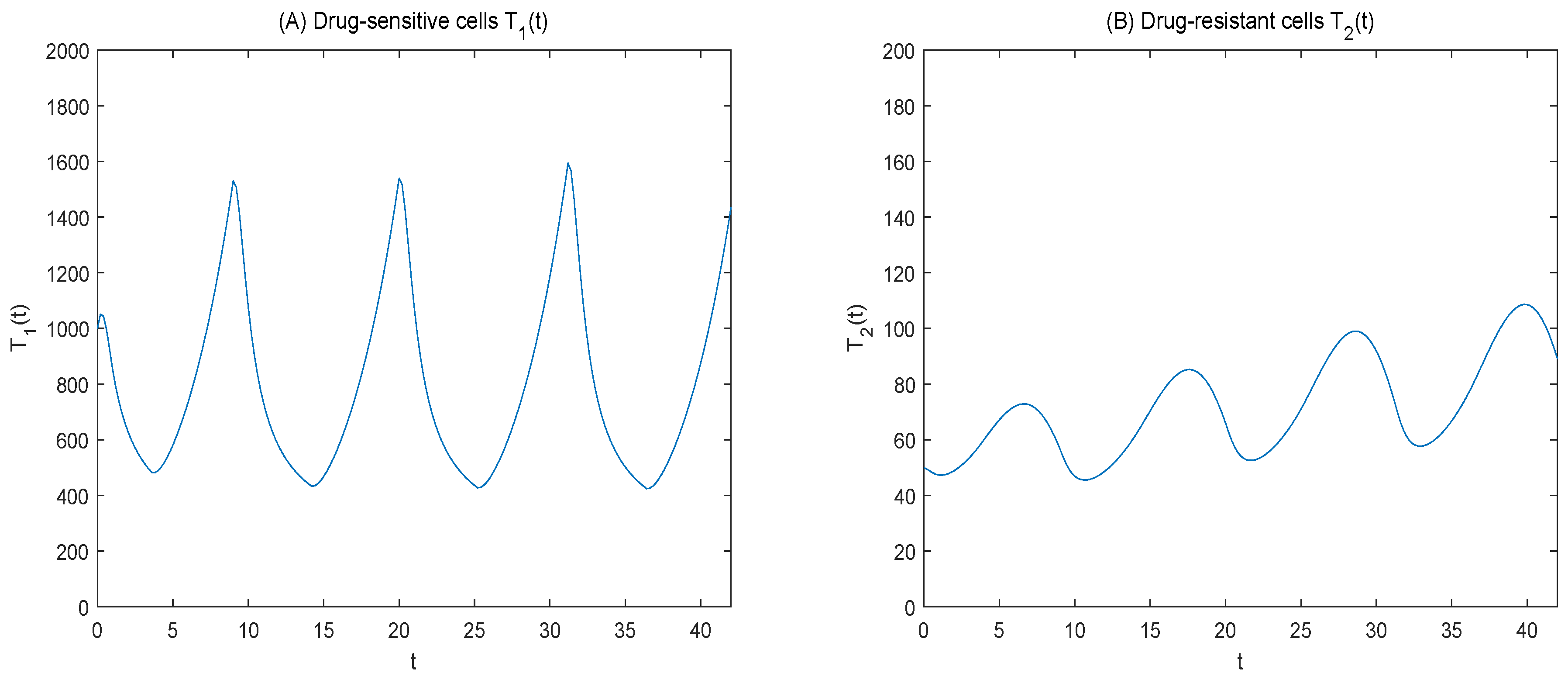
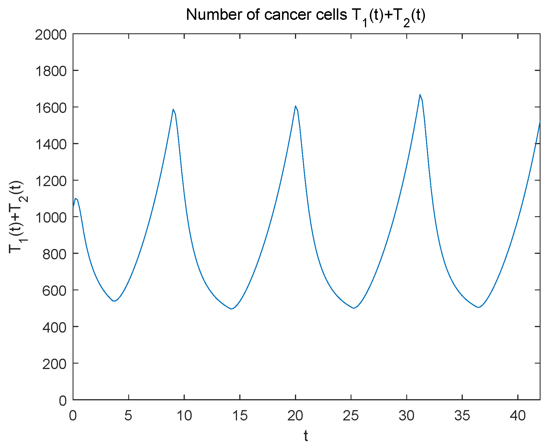
Among them, Figure 1 shows the time-varying curves for the drug concentration and drug dose, Figure 2 shows the time-varying curves for the number of sensitive versus resistant cells, and Figure 3 shows the tumor burden change curves. Using the necessary optimality condition, the terminal time covariance is obtained via the covariance equation.

$${\lambda }_1\left(t_f\right)=0,{\lambda }_2\left(t_f\right)=1,{\lambda }_3\left(t_f\right)=0,$$

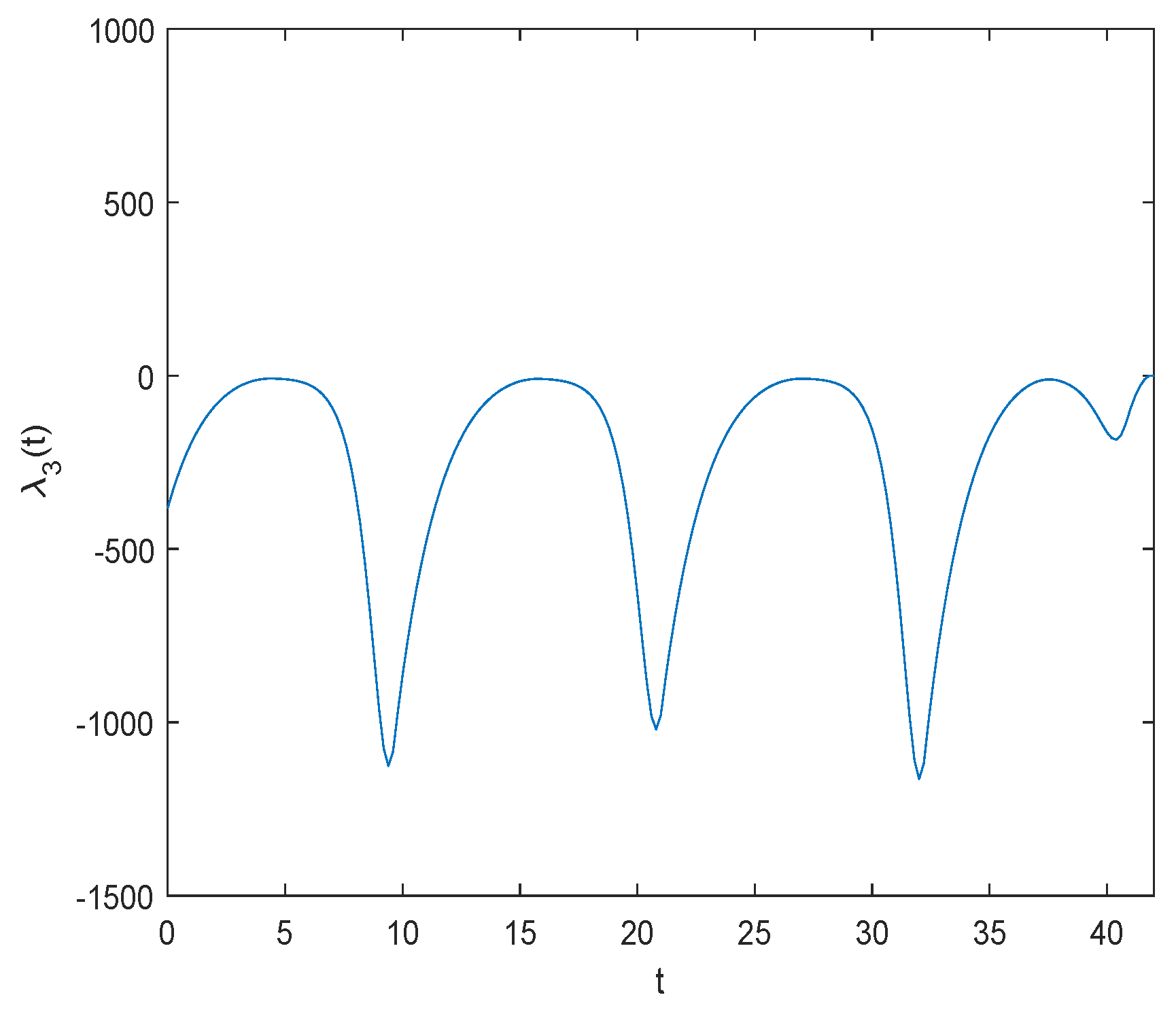
the initial value of the covariant is obtained via the numerical simulation,

$${\lambda }_1\left(0\right)=-1.2372,{\lambda }_2\left(0\right)=-8.9337,{\lambda }_3\left(0\right)=-199.7054,$$

and the adjoint variables ${\lambda }_k\left(t\right),k=1,2,3,$ are displayed in Figure 4 and Figure 5.

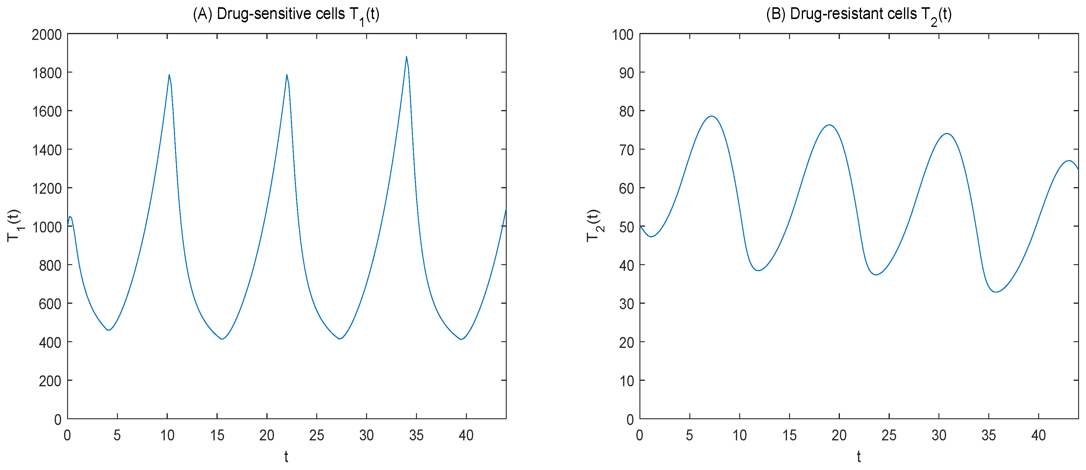
Figure 1B shows that the drug dose was initially presented at the maximum tolerated dose; when the maximum allowable drug concentration was reached, the drug dose was reduced with intermittent dosing, controlling for the number of cancer cells. Figure 2 shows that the number of sensitive cells decreased and the number of resistant cells increased after administration. After drug withdrawal, sensitive cells increased, resistant cells decreased, the number of cancer cells showed periodic changes, drug-resistant cells increased slowly with the prolongation of treatment time. Figure 3 shows that the tumor burden is maintained at a certain level.

Competition between cancer cells.

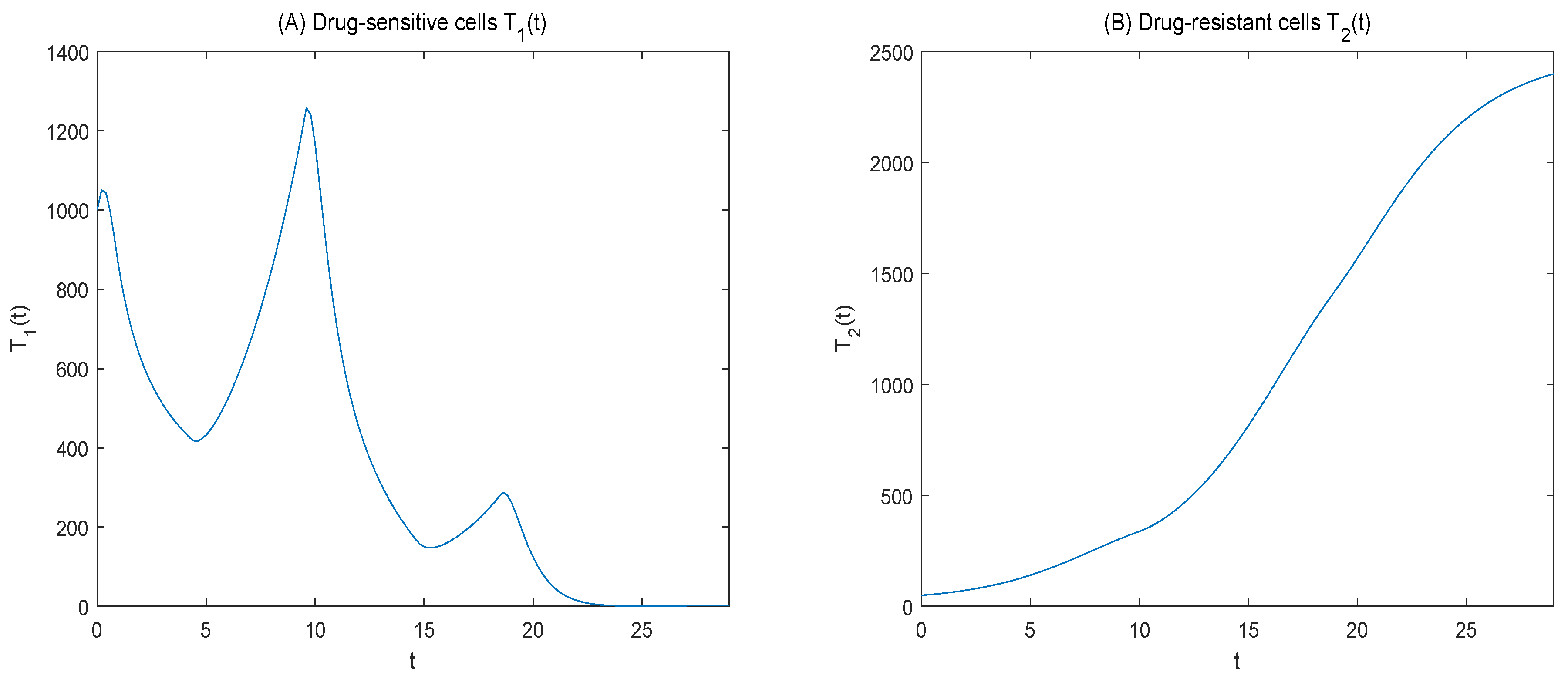
Adaptive therapy utilizes competition among cancer cells to maintain a certain tumor burden. Thus, we think more about competition between cells. When $a_{11}=0.8$, there is too much competition between sensitive cells; as shown in Figure 6, we can see that sensitive cells can inhibit drug-resistant cells during the initial phase of treatment, and the number of drug-resistant cells slowly increases. In the later period of treatment, the number of sensitive cells decreased sharply and the number of drug-resistant cells increased because of the competition between sensitive cells.

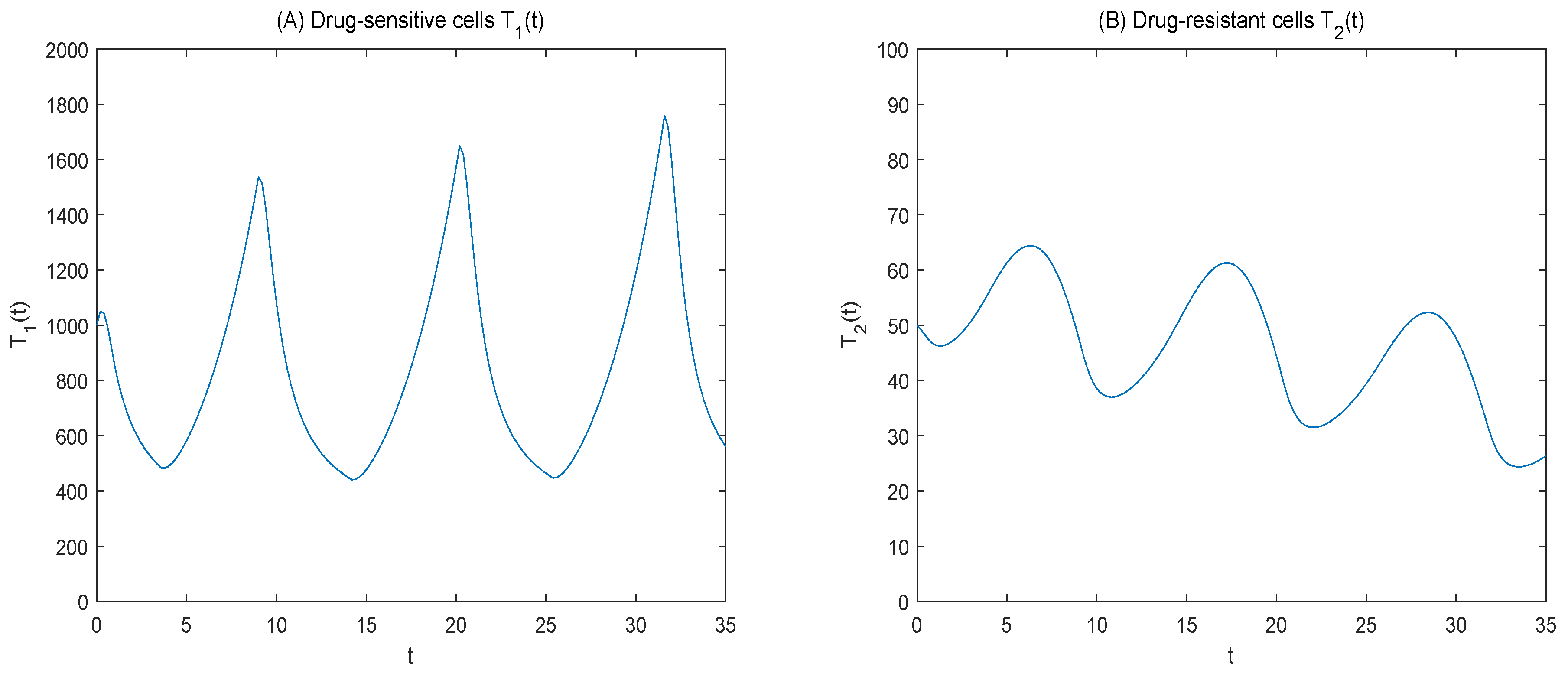
When $a_{12}=0.8$, as shown in Figure 7, we can see that at the initial stage of treatment, sensitive cells show cyclical changes, and resistant cells slowly increase; at later stages of treatment, sensitive cells lose their competitive advantage, and drug-resistant cells increase.

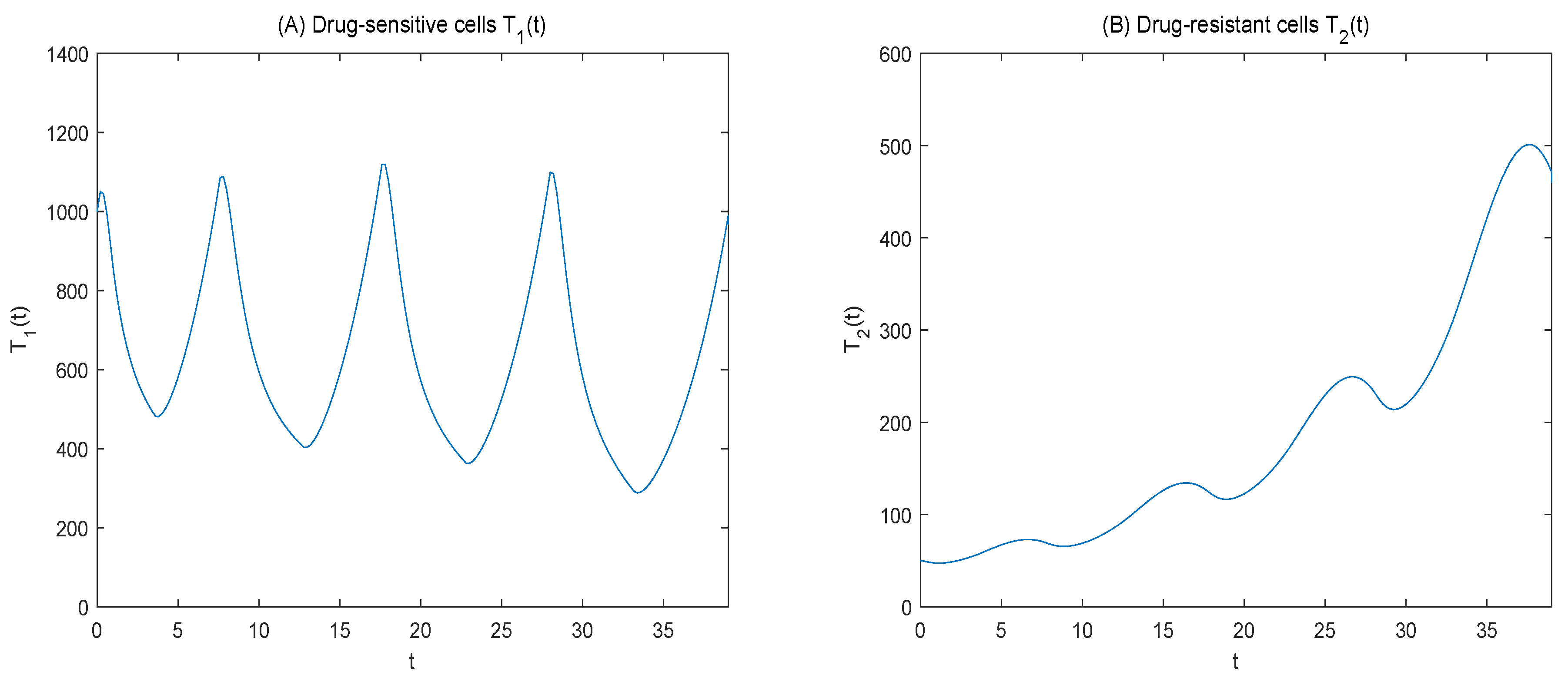
When $a_{21}=0.2$, as shown in Figure 8, we can see that sensitive cells can inhibit drug-resistant cells at the initial stage of treatment, and at the later stage of treatment, drug-resistant cells increase dramatically; compared with $a_{12}$, drug-resistant cells are more numerous, reducing the duration of treatment.

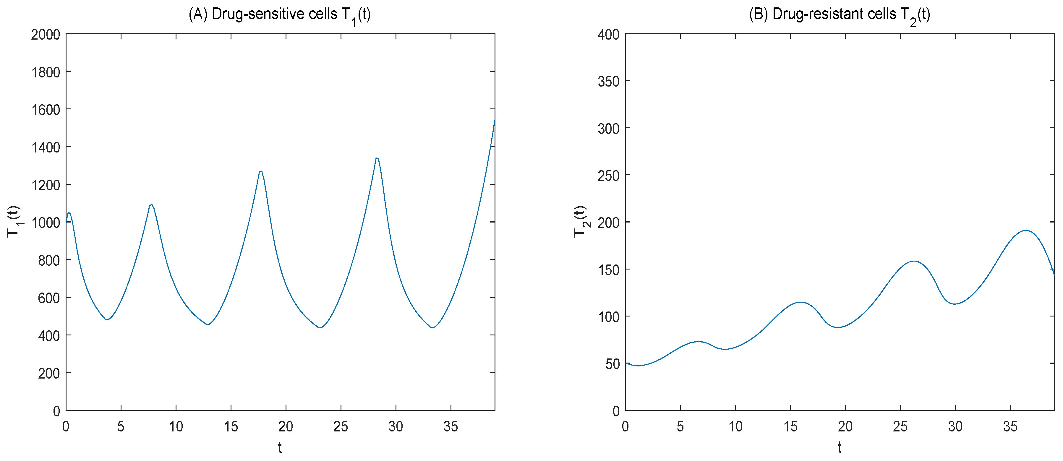
When $a_{22}=0.8$, as shown in Figure 9, it shows a downward trend in the number of drug-resistant cells but an increase in the number of sensitive cells, resulting in a rapid reach of the tumor burden and subsequent treatment failure.

Drug concentration

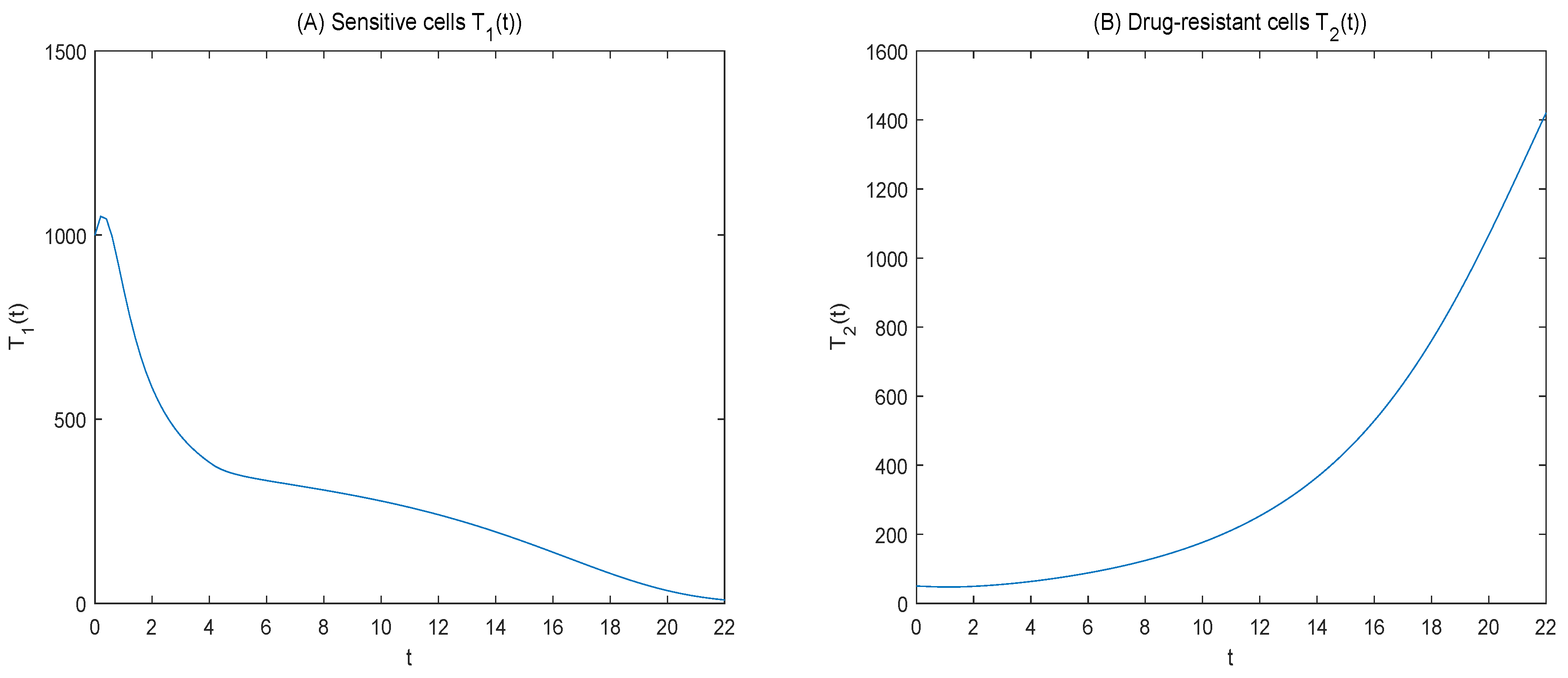
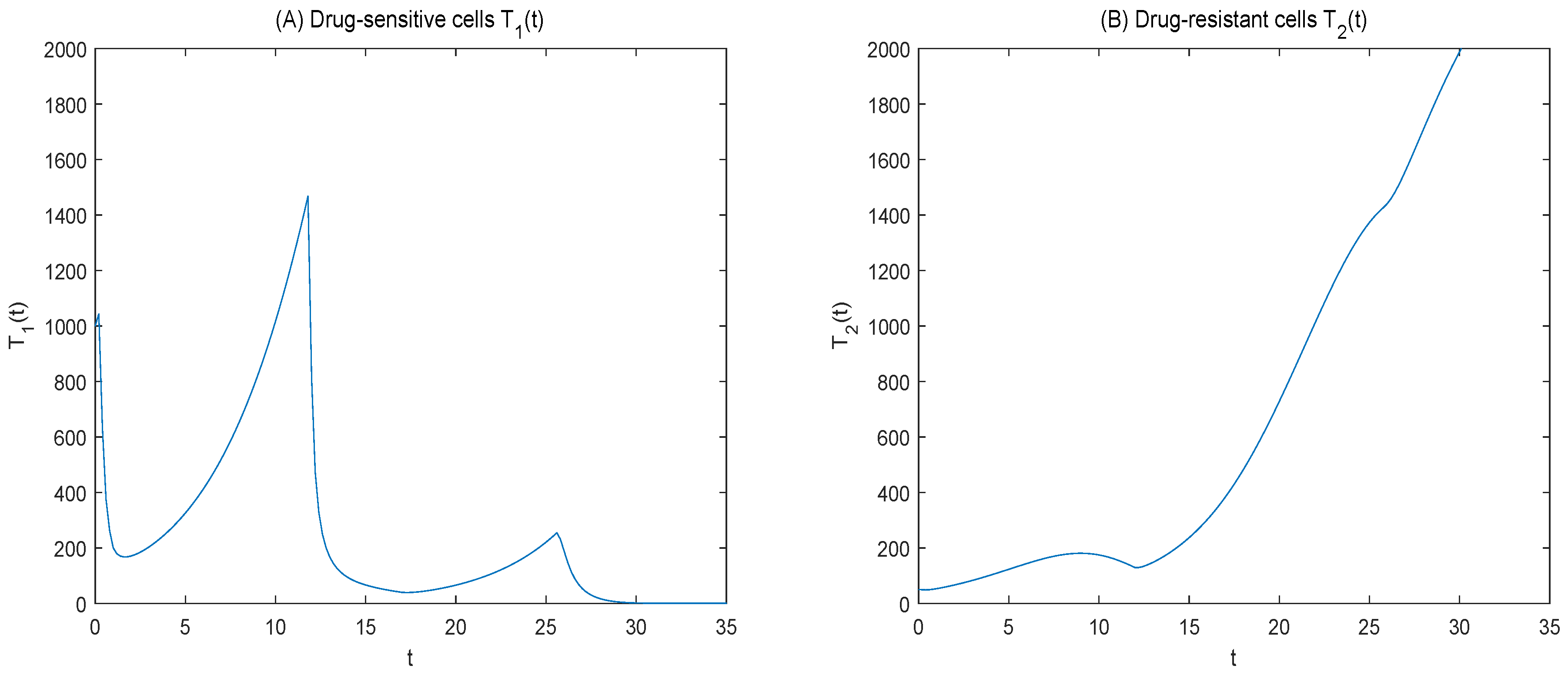
This study proposed the effect of drug concentration on therapy. We further considered the model proposed by Liu et al, considering only the effect of drug dose on therapy. Adjusting for ${\lambda }_1=0.1$, as shown in Figure 10, we found an overall upward trend in sensitive cells and a decrease in drug-resistant cells, this resulted in the sensitive cells rapidly reaching the maximum tumor burden, leading to treatment failure. The results showed that the drug was not enough to kill a large number of sensitive cells, resulting in a competitive advantage of sensitive cells over drug-resistant cells. Compared with Figure 9, we can see that the number of drug-resistant cells can be more effectively controlled and the stable tumor burden can be maintained by considering the drug concentration.

4.1. Consider the Tumor Burden as 110%

The drug dosage is unchanged and the treatment time is optimized.

Optimal treatment time.  $t_1=0.8,$$t_2=3.4,$$t_3=7.4,$$t_4=12.6,$$t_5=17.4,$$t_6=22.6,$$t_7=27.8,$$t_8=33.$

We can obtain $T_2\left(t_f\right)=471.0447,$ $J=486.1442.$

Figure 11 shows the curve of sensitive and resistant cells over time at 110% tumor burden; we can see that the killing rate of drug-sensitive cells increases with the prolongation of treatment time, and the number of drug-resistant cells shows an overall declining trend. The number of drug-resistant cells increases, which indicates that the sensitive cells do not inhibit the drug-resistant cells well in the later stage of treatment.

Compared to a starting treatment, when the tumor burden is 150%, the treatment time is shortened and more resistant cells are generated. The reason for the significant increase in the number of drug-resistant cells may be that the drug dose is too large, killing too many sensitive cells, resulting in the later period of treatment, cell-to-cell competition weakens, and the number of drug-resistant cells increases. Therefore, we further optimize the drug dose.

Drug dose. ${\beta }_1=0.7856$, ${\beta }_2=0.7$, ${\beta }_3=0.7$, ${\beta }_4=0.7.$

We can obtain $T_2\left(t_f\right)=143.3169,$ $J=157.0795.$

Changes in drug-sensitive cells affect drug-resistant cells because high doses kill too many drug-sensitive cells. Therefore, we reduce the drug dose, as shown in Figure 12, as the drug dose decreases over time. The number of drug-sensitive cells shows an upward trend, while the number of drug-resistant cells significantly decreases. Therefore, when the patient’s maximum tolerated tumor burden is small, the dose is relatively small, suppressing the number of resistant cells. However, compared with 150% tumor burden, the number of drug-resistant cells remain larger at the end of the treatment period, despite the reduced cost of the drug.

4.2. Consider the Tumor Burden as 170%

The drug dosage is unchanged and the treatment time is optimized.

Optimal treatment time  $t_1=0.8,$$t_2=3.8,$$t_3=10,$$t_4=15.2,$$t_5=21.8,$$t_6=27,$$t_7=33.8,$$t_8=39.2.$

We can obtain $T_2\left(t_f\right)=23.8859,$ $J=39.4568.$

Figure 13 shows the curve of sensitive and resistant cells over time at 170% tumor burden. It shows that the number of sensitive cells increases significantly with the time of treatment, showing an overall upward trend. The number of drug-resistant cells increases at the beginning of treatment, decrease significantly at the end of treatment, and are even lower than the initial resistant cells. This indicates that, at this time, there are too many sensitive cells and competitive enhancements of the inhibition of drug-resistant cells.

Compared to a tumor burden of 150%, the number of drug-resistant cells is significantly lower, but the number of drug-sensitive cells is significantly increased. This could cause the tumor to reach the maximum tolerable burden more quickly, resulting in treatment failure The reason for this change may be that the drug did not kill enough sensitive cells, causing the sensitive cells to grow too quickly, so we further optimize the drug dose.

Drug dose. ${\beta }_1=0.7856$, ${\beta }_2=0.84$, ${\beta }_3=0.84$, ${\beta }_4=0.84.$

We can obtain $T_2\left(t_f\right)=64.5510,$ $J=80.9798.$

To control drug-sensitive cells, we adjust the drug dose, as shown in Figure 14; as the drug dose increases, the number of sensitive cells decreases and the number of drug-resistant cells increases. As a result, the tumor burden increases and the drug dose increases. Compared with a tumor burden of 150%, during longer treatment periods, the number of drug-resistant cells is less, but the increasing dose of the drug and the rising cost of the drug, to some extent, break the limit of drug toxicity and affect normal cells.

At the same time, we further simulate the maximum tolerated dose commonly used in clinical practice.

4.3. Dose Titration Protocol

Cunningham et al. [4] analyzed a widely-used regimen, specifically a dose-titration treatment approach. In this regimen, the dose is increased by 0.1 when the tumor volume rises to more than 110% of the target tumor volume. Conversely, if the tumor volume drops below 90% of the intended maintenance volume, the dose is decreased by 0.1. They determined the optimal treatment strategy for the drug obtained using the optimization theory. With reference to the dose titration protocol described above, our study treats the number of cancer cells as the tumor burden; thus, given an initial dose, if the tumor burden increases to 150%, the dose increases by 0.1; if it decreases to 50%, the dose decreases by 0.1.

Let us think about a cycle; consider the issue of drug toxicity.

Drug dose: $b_1=0.8$, $b_2=0.7$,

Drug time: $t_1=4$, $t_2=22.2,$

We can obtain $T_2\left(t_f\right)=1595.4672,$ $J=1687.6672.$

The change in the number of cancer cells is shown in Figure 15.

As shown in Figure 15, when the initial dose is set at the maximum tolerated dose and considering the tumor burden, the number of drug-dose-sensitive cells was effectively reduced. However, due to a slow reduction in the dose, the number of drug-resistant cells increased significantly within a shorter treatment period.

Therefore, using dose titration to determine the most beneficial dose might lead to the rapid killing of sensitive cells, resulting in a loss of competitiveness. Our treatment protocol, through numerical simulation, directly provides the optimal drug dose. This controls the number of sensitive cells, inhibits the rapid proliferation of drug-resistant cells, and extends the treatment time.

Summary

The numerical simulation results show that when the tumor burden is 150%, within the permissible limit of drug toxicity, the administration of the drug causes drug-sensitive cells to decrease and drug-resistant cells to increase. Upon withdrawal of the drug, the sensitive cells increase, and the drug-resistant cells decrease. Throughout the treatment period, the number of drug-resistant cells increased slowly, and the tumor burden was maintained at a certain level. The competition between cells affects cell changes, and further analysis does not take into account the problem of drug concentration when it is not sufficient to kill sensitive cells, resulting in a significant increase in drug-resistant cells. When the tumor burden is 110%, the drug dose is reduced, the drug cost is reduced, the treatment time is shortened, and more resistant cells are produced. When the tumor load is 170%, the treatment time is prolonged, the number of drug-resistant cells is relatively small, but it is easy to reach the maximum drug-resistant load. Further increasing the drug dose will lead to breaking the limit of drug toxicity, affecting healthy cells. For dose-titration problems, given an initial dose and considering the drug toxicity issue, the strategy involves gradually increasing or decreasing the drug dose to find the most beneficial amount. When the initial dose is high, using the magnitude of the tumor burden to adjust the dose might result in extensive death of sensitive cells, a loss of competitiveness, and a significant rise in the number of drug-resistant cells. If the initial dose is low, the gradual increase in dose and failure to eliminate sensitive cells can lead to the rapid proliferation of these cells, which soon reach the maximum tolerance of the tumor load, leading to treatment failure. Therefore, the maximum tolerated tumor burden is too large or too small, and the drug dose is too large or too small, which will affect the effect of treatment. Using mathematical simulation, our study shows that the initial maximum drug resistance dose is given first; the drug is discontinued when the maximum allowable drug concentration is reached. When 150% of the initial tumor burden is reached, the drug is administered, and with the prolongation of the treatment period, it is optimal to give the drug intermittently at a moderate dose, which not only maintains a certain tumor burden and inhibits the rapid growth of drug-resistant cells, but also limits the drug toxicity and reduces the cost of the drug; the duration of treatment is prolonged effectively.

However, the maximum tolerable tumor burden varies from patient to patient, and we only considered the general case. Therefore, how to monitor the patient’s maximum tolerable tumor burden according to clinical practice is important. Choosing the optimal treatment time and dosage and implementing individualized treatments are the issues that will be studied next.

5. Conclusions

During the course of tumor treatment, the generation of drug-resistant cells leads to the failure of treatment. With adaptive therapy, the goal is to maintain a certain number of sensitive cells, competitive inhibition resistance, a certain tumor burden, and extend the duration of treatment. Therefore, it is critical to select the appropriate treatment time and drug dose. If the dose is too low, it might fail to kill enough sensitive cells, leading to the quick attainment of the maximum tolerated tumor burden. Conversely, an excessively high dose may result in the death of a large number of sensitive cells, reducing competition and inhibiting the growth of drug-resistant cells less effectively. Additionally, an accumulation of too many drugs could have adverse side effects on the body. We took into consideration the model of competition between drug-sensitive and drug-resistant cells proposed by Liu et al. [5], and introduced a pharmacokinetics equation to describe the time course of drug concentrations in vivo. Because the drug not only kills cancer cells but also has an effect on healthy ones, it is not possible to cure cancer cells in sufficient doses. Therefore, in the process of cancer treatment, the issue of drug toxicity is proposed. We look at how to achieve the ideal cancer cell-killing rate and inhibit the growth of drug-resistant cells without damaging the healthy cells, and how to select the treatment time and dose to achieve the optimal therapeutic effect. We propose optimal control problems with two state constraints: the maximum allowable drug concentration and the maximum tolerated tumor burden. Firstly, the optimal control structure was obtained by using the optimal control theory to analyze the control problems. Secondly, the optimal treatment time and drug dose were obtained by numerical simulation, and the change rule of tumor cells under different tumor loads and the optimal treatment time and drug dose were given; a dose titration protocol was further simulated. The results show that when the tumor burden is at 150%, it is optimal to administer the maximum tolerated dose. Once the maximum allowable drug concentration is attained, the drug should be given intermittently at a moderate dose. This strategy helps maintain the tumor burden at a stable level, inhibit the growth of drug-resistant cells, reduce drug costs, and prolong the drug’s efficacy. These findings offer insights into the treatment of prostate cancer.

However, our study relies on initial values while focusing on the effects of intercellular competition factors on treatment, so that initial values and competition coefficients have a greater impact on treatment outcomes than other factors. At the same time, the drug concentration change in the human body is worthy of further study. For the treatment approach proposed in this paper, determining how to tailor it to the individual patient’s situation remains a topic for a follow-up study.

References

1. Gatenby, R.A. A change of strategy in the war on cancer. Nature 2009, 459, 508–509. [Google Scholar] [CrossRef]
2. Gatenby, R.A.; Silva, A.S.; Gillies, R.J.; Frieden, B.R. Adaptive therapy. Cancer Res. 2009, 69, 4894–4903. [Google Scholar] [CrossRef]
3. Zhang, J.; Fishman, M.N.; Brown, J.; Gatenby, R.A. Integrating evolutionary dynamics into treatment of metastaticcastrate-resistant prostate cancer (mCRPC): Updated analysis of the adaptive abiraterone (abi) study (NCT02415621). J. Clin. Oncol. 2019, 37, 5041. [Google Scholar] [CrossRef]
4. Cunningham, J.; Thuijsman, F.; Peeters, R.; Viossat, Y.; Brown, J.; Gatenby, R.; Staňková, K. Optimal control to reach eco-evolutionary stability in metastatic castrate-resistant prostate cancer. PLoS ONE 2020, 15, e0243386. [Google Scholar] [CrossRef]
5. Liu, R.; Wang, S.; Tan, X.; Zou, X. Identifying optimal adaptive therapeutic schedules for prostate cancer through combining mathematical modeling and dynamic optimization. Appl. Math. Model. 2022, 107, 688–700. [Google Scholar] [CrossRef]
6. West, J.B.; Dinh, M.N.; Brown, J.S.; Zhang, J.; Anderson, A.R.; Gatenby, R.A. Multidrug cancer therapy in metastatic castrate-resistant prostate cancer: An evolution-based strategy. Clin. Cancer Res. 2019, 25, 4413–4421. [Google Scholar] [CrossRef]
7. Strobl, M.A.R.; West, J.; Viossat, Y.; Damaghi, M.; Robertson-Tessi, M.; Brown, J.S.; Gatenby, R.A.; Maini, P.K.; Anderson, A.R. Turnover modulates the need for a cost of resistance in adaptive therapy. Cancer Res. 2021, 81, 1135–1147. [Google Scholar] [CrossRef]
8. Ledzewicz, U.; Schättler, H. Optimal controls for a model with pharmacokinetics maximizing bone marrow in cancer chemotherapy. Math. Biosci. 2007, 206, 320–342. [Google Scholar] [CrossRef]
9. Ledzewicz, U.; Maurer, H.; Schättler, H. Optimal and suboptimal protocols for a mathematical model for tumor anti-angiogenesis in combination with chemotherapy. Math. Biosci. Eng. 2011, 8, 307–323. [Google Scholar]
10. Iliadis, A.; Barbolosi, D. Optimizing drug regimens in cancer chemotherapy by an efficacy-toxicity mathematical model. Comput. Biomed. Res. 2000, 33, 211–226. [Google Scholar] [CrossRef]
11. Tan, P.L.; Maurer, H.; Kanesan, J.; Chuah, J.H. Optimal Control of Cancer Chemotherapy with Delays and State Constraints. J. Optim. Theory Appl. 2022, 194, 749–770. [Google Scholar] [CrossRef]
12. Hansen, E.; Read, A.F. Modifying adaptive therapy to enhance competitive suppression. Cancers 2020, 12, 3556. [Google Scholar] [CrossRef]
13. Göllmann, L.; Kern, D.; Maurer, H. Optimal control problems with delays in state and control variables subject to mixed control-state constraints. Optim. Control Appl. Methods 2009, 30, 341–365. [Google Scholar] [CrossRef]
14. Göllmann, L.; Maurer, H. Theory and applications of optimal control problems with multiple time-delays. J. Ind. Manag. Optim. 2014, 10, 413–441. [Google Scholar] [CrossRef]
15. Büskens, C.; Maurer, H. SQP-methods for solving optimal control problems with control and state constraints: Adjoint variables, sensitivity analysis and real-time control. J. Comput. Appl. Math. 2000, 120, 85–108. [Google Scholar] [CrossRef]
16. Tan, J.; Zou, X. Optimal control strategy for abnormal innate immune response. Comput. Math. Methods Med. 2015, 2015, 386235. [Google Scholar] [CrossRef] [PubMed]
17. Li, S.; Zhao, R.; Zhang, Q. Optimization method for solving bang-bang and singular control problems. J. Control Theory Appl. 2012, 10, 559–564. [Google Scholar] [CrossRef]
18. Yang, F.; Teo, K.L.; Loxton, R.; Rehbock, V.; Li, B.; Yu, C.; Jennings, L. VISUAL MISER: An efficient user-friendly visual program for solving optimal control problems. J. Ind. Manag. Optim. JIMO 2016, 12, 781–810. [Google Scholar]
19. Maurer, H.; Büskens, C.; Kim, J.H.R.; Kaya, C.Y. Optimization methods for the verification of second order sufficient conditions for bang-bang controls. Optim. Control Appl. Methods 2005, 26, 129–156. [Google Scholar] [CrossRef]
20. Kaya, C.Y.; Noakes, J.L. Computational method for time-optimal switching control. J. Optim. Theory Appl. 2003, 117, 69–92. [Google Scholar] [CrossRef]
21. Lee, H.W.J.; Teo, K.L.; Rehbock, V.; Jennings, L.S. Control parametrization enhancing technique for time optimal control problems. Dyn. Syst. Appl. 1997, 6, 243–262. [Google Scholar]
Figure 1. (A) Denotes the drug concentration, (B) denotes the drug dose.
Mathematics 11 04025 g001
Figure 2. (A) Denotes the drug-sensitive cells, (B) denotes the drug-resistant cells (tumor burden is 150%).
Mathematics 11 04025 g002
Figure 3. Number of cancer cells.
Mathematics 11 04025 g003
Figure 4. (A) Denotes adjoint variables λ 1 , (B) denotes adjoint variables λ 2 .
Mathematics 11 04025 g004
Figure 5. Denotes adjoint variables λ 3 .
Mathematics 11 04025 g005
Figure 6. (A) Denotes drug-sensitive cells, (B) denotes drug-resistant cells (when a 11 = 0.8 ).
Mathematics 11 04025 g006
Figure 7. (A) Denotes drug-sensitive cells, (B) denotes drug-resistant cells (when a 12 = 0.8 ).
Mathematics 11 04025 g007
Figure 8. (A) Denotes drug-sensitive cells, (B) denotes drug-resistant cells (when a 21 = 0.2 ).
Mathematics 11 04025 g008
Figure 9. (A) Denotes drug-sensitive cells, (B) denotes drug-resistant cells (when a 22 = 0.8 ).
Mathematics 11 04025 g009
Figure 10. (A) Denotes drug-sensitive cells, (B) denotes drug-resistant cells.
Mathematics 11 04025 g010
Figure 11. (A) Denotes drug-sensitive cells, (B) denotes drug-resistant cells (tumor burden is 110%).
Mathematics 11 04025 g011
Figure 12. (A) Denotes drug-sensitive cells, (B) denotes drug-resistant cells (tumor burden is 110%).
Mathematics 11 04025 g012
Figure 13. (A) Denotes drug-sensitive cells, (B) denotes drug-resistant cells (tumor burden is 170%).
Mathematics 11 04025 g013
Figure 14. (A) Denotes drug-sensitive cells, (B) denotes drug-resistant cells (tumor burden is 170%).
Mathematics 11 04025 g014
Figure 15. (A) Denotes drug-sensitive cells, (B) denotes drug-resistant cells (dose titration protocol).
Mathematics 11 04025 g015
Disclaimer/Publisher’s Note: The statements, opinions and data contained in all publications are solely those of the individual author(s) and contributor(s) and not of MDPI and/or the editor(s). MDPI and/or the editor(s) disclaim responsibility for any injury to people or property resulting from any ideas, methods, instructions or products referred to in the content.