Ratio Test for Mean Changes in Time Series with Heavy-Tailed AR(p) Noise Based on Multiple Sampling Methods

Abstract

This paper discusses the problem of the mean changes in time series with heavy-tailed AR(p) noise. Firstly, it proposes a modified ratio-type test statistic, and the results show that under the null hypothesis of no mean change, the asymptotic distribution of the modified statistic is a functional of Lévy processes and the consistency under the alternative hypothesis is obtained. However, a heavy-tailed index exists in the asymptotic distribution and is difficult to estimate. This paper uses bootstrap sampling, jackknife sampling, and subsampling to approximate the distribution under the null hypothesis, and obtain more accurate critical values and empirical power. In addition, some results from a small simulation study and a practical example give an idea of the finite sample behavior of the proposed statistic.

1. Introduction and Statistical Framework

The problem of detecting change points in real data series has attracted attention due to the heterogeneities of real data series. The aim of change point detection and estimation is to partition data sequences into multiple homogeneous segments, and the theories have been applied in a variety of fields such as finance [1], medicine [2], the environment [3], and so on. Traditionally, change point problems are generally described as typical hypothesis testing problems. What most scholars are interested in is testing the null hypothesis that all observations are samples from distributions with equal means, then, deriving the distributions of the statistics (see [4,5,6,7,8]). A similar reasoning holds for other change point problems, such as variance change points [9].

In the past 40 years, new models have continuously been established for more precise descriptions of financial data. Many empirical studies have shown that the phenomenon of heavy tails frequently exists in economic and financial sequences, but most previous studies have been based on finite variance (see Guillaume et al. [10] and Mittnik and Rachev [11]), and there have been few simulations using infinite variance processes. In the case of infinite variance, there will be more factors to consider and the problem will be more complex. Qin et al. [12] proposed a modified ratio test statistic that can effectively detect changes in the second half of the observed values, and established the asymptotic properties under the null and alternative hypotheses. Then, Jin et al. [13] also proposed a modified ratio statistic to test the possible trend term changes in the sequences and, based on the subsampling method, more accurate critical values were obtained.

In the change point problems of heavy-tailed sequences, due to the influence of extreme values in heavy-tailed sequences, it is generally not possible to directly locate the critical value of the test statistic. Therefore, this paper proposes using multiple resampling methods to approximate the distribution of the original statistic and obtain accurate critical values and power, then comparing and analyzing the performance of these sampling methods.

As for the error terms in some models, many scholars default to the error terms being independently and identically distributed. As Aue and Horváth [14] commented in a review paper, many methods were initially developed for independent observation. But the concept of simple independent observation models is very narrow, and most real sequences do not satisfy such models. Therefore, we would like to consider more general weakly dependent cases, such as the autoregressive model. The latest research and applications can be found in [15,16,17], and this classic model will not be introduced too much here.

So, this paper discusses the problem of mean changes in time series with heavy-tailed AR(p) errors. More specifically, observations $X_1,X_2,\cdots ,X_n$, which conform to the following structure:

$$X_t=\mu +e_t,t=p+1,p+2,\cdots ,n,$$

(1)

$$e_t={\rho }_1{e}_{t-1}+{\rho }_2{e}_{t-2}+\cdots +{\rho }_p{e}_{t-p}+{\eta }_t,$$

(2)

where $\mu$ is a constant, ${\rho }_1,{\rho }_2,\cdots$ are coefficients, and ${\eta }_t$ is a heavy-tailed sequence.

Remark 1.

A heavy-tailed distribution is a special type of distribution in statistics, where the probability of the tail (i.e., extreme case) is greater than that of a normal distribution. This means that in actual observational data, the distribution is more likely to exhibit extreme and far off average values than a normal distribution.

There are two main characteristics of heavy-tailed sequences: firstly, the probability decay rate of the tail is slow; and secondly, the variance of the tail may be infinite. Common heavy-tailed distributions include the Pareto distribution, the Cauchy distribution, the t-distribution, etc. These characteristics will be implied in the assumptions in the next section.

The rest of the paper is arranged as follows: The main ideas for constructing the test statistic are detailed in Section 2. The main results are presented in Section 3. A small simulation study under different parameters is provided in Section 4. A real example is provided in Section 5. Section 6 contains the conclusions and outlooks.

2. Main Ideas

Assumption 1.

All the characteristic roots of $\rho \left(z\right)=1-{\rho }_{1}z-{\rho }_2{z}^2-\cdots -{\rho }_p{z}^p=0$ lie outside the unit circle.

Assumption 2.

${\eta }_t$ lies in the domain of attraction of a stable law with a heavy-tailed index $\kappa \in (1,2)$, and $E{\eta }_t=0$.

Remark 2.

Assumptions 1 and 2 guarantee that the heavy-tailed AR(p) sequence is smooth and has infinite variance; they are necessary underlying assumptions.

In addition, Assumption 2 implies

$$nP\left(\right|{\eta }_t|>a_{n}x)\to x^{-\kappa },$$

(3)

where $a_n=\inf \{x:P(|{\eta }_t|>x)\le n^{-1}\}$ and

$$\underset{x\to \infty }{\lim }\frac{P({\eta }_t>x)}{P\left(\right|{\eta }_t|>x)}=q\in (0,1).$$

(4)

It is not difficult to find that, by combining Equations (3) and (4), there is a constant $b_n$ such that

$$a_n^{-1}\sum _{t=1}^n({\eta }_t-b_n)\stackrel{d}{\to }{S}_k,$$

(5)

where $S_k$ is a stable random variable. In addition, it can be verified that in the special cases of $\kappa =2$ and $\kappa =1$, $S_k$ is a Gaussian and Cauchy distribution, respectively. Here, if we assume that $b_n=0$, it implies that $E{\eta }_t=0$ in Assumption 2. As a special case, if ${\eta }_t$ is an independent and identically distributed sequence, Kokoszka [18] obtained the following:

$$\left(a_n^{-1}\sum _{t=1}^{\lfloor nr\rfloor }{\eta }_t,a_n^{-2}\sum _{t=1}^{\lfloor nr\rfloor }{\eta }_t^2\right)\stackrel{d}{\to }\left(L_1\left(r\right),L_2\left(r\right)\right),$$

(6)

where $L_1\left(r\right)$ and $L_2\left(r\right)$ are κ-stable and $\kappa /2$-stable Lévy processes in the space $D[0,1]$ with the Skorohod topology, respectively. It is worth noting that $a_n$ can be rewritten as $a_n=n^{1/k}L\left(n\right)$; $L(·)$ is a slowly changing function.

Since the characteristic roots are outside the unit circle, then B–N (Beveridge–Nelson) decomposition can be used to rewrite the partial sum of $e_t$ as

$$a_n^{-1}\sum _{t=1}^{\lfloor nr\rfloor }{e}_t=D\left(1\right)a_n^{-1}\sum _{t=1}^{\lfloor nr\rfloor }{\eta }_t+a_n^{-1}({\tilde{\eta }}_0-{\tilde{\eta }}_{\lfloor nr\rfloor }),$$

(7)

where $D\left(L\right)={(1-{\rho }_{1}L-{\rho }_2{L}^2-\cdots -{\rho }_p{L}^p)}^{-1}:={\sum }_{j=0}^p{d}_j{L}^j$, ${\tilde{\eta }}_t:={\sum }_{j=0}^{\infty }\left({\sum }_{s=j+1}^{\infty }{d}_s\right){\eta }_{t-j}$.

Remark 3.

$L_1(·)$ is a stationary process that can be expressed as:

$$L_1\left(v\right)=\left\{\begin{array}{ccc}\sum _{j=1}^{\infty }{\delta }_j{\mathrm{\Gamma }}_j^{-1/\kappa }I(U_j\le v),\hfill & \hfill & \kappa \in (1,2),\hfill \\ W\left(v\right),\hfill & \hfill & \kappa =2.\hfill \end{array}\right.$$

(8)

where $W\left(v\right)$ is a standard Brownian motion. $\left\{U_j\right\}$ is a uniformly distributed random variable independently and identically distributed on the interval $[0,1]$, $\left\{{\delta }_j\right\}$ is an independently and identically distributed random variable sequence with $P({\delta }_j=1)=p$; $P({\delta }_j=-1)=1-p$. ${\mathrm{\Gamma }}_1$, ${\mathrm{\Gamma }}_2$, ⋯ are the arrival times of the Poisson process with the Lebesgue measure, and $\{U_j,{\delta }_j,{\mathrm{\Gamma }}_j\}$ are independent of each other.

Observation $X_t$ can be rewritten as

$$X_t=\mu +{\Delta }_{1}I(k^{*}<t<n)+e_t,$$

(9)

where $e_t$ is defined by (1), $\mu$ is the mean, $k^{*}$ is the time point of abrupt change, and $I(·)$ is characteristic function. The null hypothesis for testing the change is

$$H_0:k^{*}=n,$$

against the alternative hypothesis

$$H_1:k^{*}<n.$$

Shao [19] proposed a ratio test to detect the mean change point.

$$\mathrm{\Xi }=\underset{n{v}_1\le k\le n{v}_2}{\max }R\left(k\right),$$

$$R\left(k\right)=\frac{n\left|{\overline{X}}_{1,k}-{\overline{X}}_{k+1,n}\right|}{n^{-1/2}{\left\{{\sum }_{i=1}^k{\left[{\sum }_{j=1}^i(X_j-{\overline{X}}_{1,k})\right]}^2+{\sum }_{i=k+1}^n{\left[{\sum }_{j=1}^i(X_j-{\overline{X}}_{k+1,n})\right]}^2\right\}}^{1/2}},$$

where ${\overline{X}}_{m,n}={(n-m+1)}^{-1}{\sum }_{t=m}^n{X}_t$.

When dealing with the mean change point problem for heavy-tailed sequences, it is common to choose to intercept some part of the sequence for processing. Often, it is desirable to retain a large portion of the data while effectively minimizing the effect of extreme values. So, the truncated parameters are set to $(v_1,v_2)=(0.2,0.8)$.

The statistic is not actually directly substitutable into the change point model presented in this paper. The reason is the limiting distribution of $a_n^{-1}{\sum }_{t=1}^{\lfloor nr\rfloor }{e}_t$ is not available under the case of $H_0$. To solve this resistance, we suggest using ${\eta }_t$ instead of $X_t$ and re-establishing the test statistics. Because of the heavy-tail feature of ${\eta }_t$, the new test statistics are based on the residual error ${\hat{\eta }}_t$. The improved ratio tests are as follows:

$${\mathrm{\Xi }}_1=\underset{n{v}_1\le k\le n{v}_2}{\max }{R}_1\left(k\right),$$

$$\begin{array}{cc}\hfill & R_1\left(k\right)=\hfill \\ \hfill & \frac{\left|{\sum }_{t=p+1}^k({\hat{\eta }}_{0,t}-{\overline{\hat{\eta }}}_{0,(p+1,n)})\right|}{n^{-1/2}{\left\{{\sum }_{i=p+1}^k{\left[{\sum }_{t=p+1}^i({\hat{\eta }}_{1,t}-{\overline{\hat{\eta }}}_{1,(p+1,k)})\right]}^2+{\sum }_{i=k+p+1}^n{\left[{\sum }_{t=k+p+1}^i({\hat{\eta }}_{2,t}-{\overline{\hat{\eta }}}_{2,(k+p+1,n)})\right]}^2\right\}}^{1/2}},\hfill \end{array}$$

where ${\overline{\hat{\eta }}}_{i,(m,n)}={(n-m+1)}^{-1}{\sum }_{t=m}^n{\hat{\eta }}_{i,t}$. The process of obtaining ${\hat{\eta }}_{0,t}$ is not difficult. First, use the regression of $X_t$ on the intercept to calculate the ordinary least squares residual ${\hat{e}}_{0,t}$. Then, repeating the same method, calculate the residual ${\hat{\eta }}_{0,t}$ from the regression of ${\hat{e}}_{0,t}$ on ${\hat{e}}_{0,t-j}$, where $j=1,\cdots ,p$, $t=p+1,\cdots ,n$. Similarly, ${\hat{\eta }}_{1,t}$ and ${\hat{\eta }}_{2,t}$ can be obtained in ${\left\{X_t\right\}}_{t=p+1}^k$ and ${\left\{X_t\right\}}_{t=k+1}^n$, respectively.

3. Asymptotic Results

This section gives the limit distribution of the test statistic under the null hypothesis and the consistency under the alternative hypothesis. Let $v=k/n$, $s=i/n$, $v^{*}=k^{*}/n$, then we obtain Theorem 1:

Theorem 1.

Let $X_t$ be defined by (9). If the null hypothesis is true and $X_t$ satisfies Assumptions 1 and 2, when $n\to \infty$,

$${\mathrm{\Xi }}_1\stackrel{d}{\to }\underset{v_1^{*}\le v\le v_2^{*}}{\sup }\frac{\left|V\right(v;0,1\left)\right|}{{\left\{{\int }_0^v{V}^2(s;0,v)ds+{\int }_v^1{V}^2(s;v,1)ds\right\}}^{1/2}},$$

$V(a;b,c)$ is defined as: $V(a;b,c)=L_1\left(a\right)-L_1\left(b\right)-(a-b){(c-b)}^{-1}(L_1\left(c\right)-L_1\left(b\right))$, where $0\le b\le a\le c\le 1$.

Proof of Theorem 1.

Considering a prior claim about the first term in the denominator. First, using ordinary least squares (OLS), calculate the residual ${\hat{e}}_{1,t}=X_t-k^{-1}{\sum }_{t=1}^k{X}_t=e_t-k^{-1}{\sum }_{t=1}^k{e}_t:=e_t-\dot{e}$ according to the expression of $X_t$ in (9). Therefore, we can rewrite ${\hat{e}}_{1,t}$.

$${\hat{e}}_{1,t}=e_t-\dot{e}={\rho }_1{\hat{e}}_{1,t-1}+\cdots +{\rho }_p{\hat{e}}_{1,t-p}+{\hat{\xi }}_t,$$

(10)

where ${\hat{\xi }}_t=({\rho }_1+\cdots +{\rho }_p-1)\dot{e}+{\eta }_t$, $t=p+1$, ⋯, k.

Let $\theta ={({\rho }_1,{\rho }_2,\cdots ,{\rho }_p)}^{\top },\hat{\xi }={({\hat{\xi }}_{p+1},\cdots ,{\hat{\xi }}_k)}^{\top }$,

$$\hat{e}=\left[\begin{array}{ccccc}{\hat{e}}_{1,p}& {\hat{e}}_{1,p-1}& {\hat{e}}_{1,p-2}& \cdots & {\hat{e}}_{1,1}\\ {\hat{e}}_{1,p+1}& {\hat{e}}_{1,p}& {\hat{e}}_{1,p-1}& \cdots & {\hat{e}}_{1,2}\\ {\hat{e}}_{1,p+2}& {\hat{e}}_{1,p+1}& {\hat{e}}_{1,p}& \cdots & {\hat{e}}_{1,3}\\ \cdots & \cdots & \cdots & \cdots & \cdots \\ {\hat{e}}_{1,k-1}& {\hat{e}}_{1,k-2}& {\hat{e}}_{1,k-3}& \cdots & {\hat{e}}_{1,k-p}\end{array}\right].$$

(11)

At this point, we let $G=({\hat{e}}_{1,p+1},{\hat{e}}_{1,p+2},\cdots ,{\hat{e}}_{1,k})$. Then, combined with (10), we can obtain

$$G=\hat{e}\theta +\hat{\xi }.$$

Therefore, using OLS again we can obtain

$$\hat{\theta }-\theta ={\left({\hat{e}}^{\top }\hat{e}\right)}^{-1}{\hat{e}}^{\top }\hat{\xi }.$$

where ${\hat{e}}^{\top }\hat{\xi }={\left({\sum }_{t=p}^{k-1}{\hat{e}}_{1,t}{\hat{\xi }}_{t+1},{\sum }_{t=p}^{k-2}{\hat{e}}_{1,t}{\hat{\xi }}_{t+2},\cdots ,{\sum }_{t=p}^{k-p}{\hat{e}}_{1,t}{\hat{\xi }}_{t+p}\right)}^{\top }$ and

$${\hat{e}}^{\top }\hat{e}=\left[\begin{array}{ccccc}\sum _{t=p}^{k-1}{\hat{e}}_{1,t}{\hat{e}}_{1,t}& \sum _{t=p}^{k-1}{\hat{e}}_{1,t}{\hat{e}}_{1,t-1}& \sum _{t=p}^{k-1}{\hat{e}}_{1,t}{\hat{e}}_{1,t-2}& \cdots & \sum _{t=p}^{k-1}{\hat{e}}_{1,t}{\hat{e}}_{1,t-p+1}\\ \sum _{t=p-1}^{k-2}{\hat{e}}_{1,t}{\hat{e}}_{1,t+1}& \sum _{t=p-1}^{k-2}{\hat{e}}_{1,t}{\hat{e}}_{1,t}& \sum _{t=p-1}^{k-2}{\hat{e}}_{1,t}{\hat{e}}_{1,t-1}& \cdots & \sum _{t=p-1}^{k-2}{\hat{e}}_{1,t}{\hat{e}}_{1,t-p+2}\\ \sum _{t=p-2}^{k-3}{\hat{e}}_{1,t}{\hat{e}}_{1,t+2}& \sum _{t=p-2}^{k-3}{\hat{e}}_{1,t}{\hat{e}}_{1,t+1}& \sum _{t=p-2}^{k-3}{\hat{e}}_{1,t}{\hat{e}}_{1,t}& \cdots & \sum _{t=p-2}^{k-3}{\hat{e}}_{1,t}{\hat{e}}_{1,t-p+3}\\ \cdots & \cdots & \cdots & \cdots & \cdots \\ \sum _{t=1}^{k-p}{\hat{e}}_{1,t}{\hat{e}}_{1,t+p-1}& \sum _{t=1}^{k-p}{\hat{e}}_{1,t}{\hat{e}}_{1,t+p-2}& \sum _{t=1}^{k-p}{\hat{e}}_{1,t}{\hat{e}}_{1,t+p-3}& \cdots & \sum _{t=1}^{k-p}{\hat{e}}_{1,t}{\hat{e}}_{1,t}\end{array}\right].$$

Phillips proved the following fact in Theorem 3.19 of [20]: For all j, $a_n^{-1}{\sum }_{t=1}^{n·}{e}_t=O_p\left(1\right)$ and $a_n^{-2}{\sum }_{t=1}^{n·}{e}_t{e}_{t-j}=O_p\left(1\right)$ are valid. After basic calculation, we can obtain

$$\dot{e}=O_p\left(a_n{n}^{-1}\right)$$

and

$$\sum _{t=p}^{k-1}{\hat{e}}_{1,t}{\hat{e}}_{1,t-j}=\sum _{t=p}^{k-1}(e_t-\dot{e})(e_{t-j}-\dot{e})=O_p\left(a_n^2\right)+O_p\left(a_n^2{n}^{-1}\right)=O_p\left(a_n^2\right),j=0,\cdots ,p-1.$$

(12)

Other elements in the matrix ${\hat{e}}^{\top }\hat{e}$ can be treated similarly, and their convergence rate is $O_p\left(a_n^2\right)$. Therefore, we will only consider the convergence rate of the first element in matrix ${\hat{e}}^{\top }\hat{\xi }$. Using B–N decomposition, ${\hat{e}}_{1,t}$ can be rewritten as ${\hat{e}}_{1,t}={\sum }_{s=0}^{\infty }{d}_s{\hat{\xi }}_{1,t-s}$, where ${\sum }_{s=0}^{\infty }{d}_s<\infty$.

Combining ${\hat{\xi }}_t=({\rho }_1+\cdots +{\rho }_p){\dot{e}}_t+{\eta }_t$, then we can obtain that

$$\sum _{t=p}^{k-1}{\hat{e}}_{1,t}{\hat{\xi }}_{t+1}=\sum _{t=p}^{k-1}\sum _{s=0}^{\infty }{d}_s{\hat{\xi }}_{t-s}{\hat{\xi }}_{t+1}=\sum _{s=0}^{\infty }{d}_s\sum _{t=p}^{k-1}{\eta }_{t-s}{\eta }_{t+1}+O_p\left(a_n^2{n}^{-1}\right)=O_p\left(a_n\right).$$

(13)

Owing to ${\eta }_{t+1}$ being independent of ${\eta }_{t-s}$, ${\eta }_{t+1}{\eta }_{t-s}\in D\left(\kappa \right)$, i.e., ${\sum }_{t=p}^{k-1}{\eta }_{t+1}{\eta }_{t-s}=O_p\left(a_n\right)$. Let

$$A=\left[\begin{array}{ccc}{a}_n^{-1}& & \\ & a_n^{-1}& \\ & & \ddots \\ & & & a_n^{-1}\end{array}\right],$$

(14)

Combining (12) and (13),

$$\hat{\theta }-\theta =A{\left(A{\hat{e}}^{\top }\hat{e}A\right)}^{-1}A{\hat{e}}^{\top }\hat{\xi }={[O_p\left(a_n^{-1}\right),O_p\left(a_n^{-1}\right),\cdots ,O_p\left(a_n^{-1}\right)]}^{\top }.$$

(15)

Then, for $t=p+1,\cdots ,k$,

$$\begin{array}{cc}\hfill {\hat{\eta }}_{1,t}=& {\hat{e}}_{1,t}-({\hat{\rho }}_1{\hat{e}}_{1,t-1}+{\hat{\rho }}_2{\hat{e}}_{1,t-2}+\cdots +{\hat{\rho }}_p{\hat{e}}_{1,t-p})\hfill \\ \hfill =& \sum _{l=1}^p({\rho }_l-{\hat{\rho }}_l){\hat{e}}_{1,t-l}+({\rho }_1+{\rho }_2+\cdots +{\rho }_p-1)\dot{e}+{\eta }_t.\hfill \end{array}$$

(16)

It is not difficult to see that

$$\sum _{t=1}^{[n·]}{\hat{e}}_{1,t}=\sum _{t=1}^{[n·]}(e_t+\dot{e})=O_p\left(a_n\right).$$

(17)

Let $i=\left[ns\right]$, $k=\left[nv\right]$, where $0<s,v<1$. Due to the independence of ${\eta }_t$ and Assumption 2, we combine (15), (16) and (17), then

$$\begin{array}{cc}\hfill & a_n^{-1}\sum _{t=p+1}^i({\hat{\eta }}_{1,t}-{\overline{\hat{\eta }}}_{1,(p+1,k)})\hfill \\ \hfill =& a_n^{-1}\sum _{t=p+1}^i{\eta }_t-(i-p){(k-p)}^{-1}{a}_n^{-1}\sum _{t=p+1}^k{\eta }_t+o_p\left(1\right)\stackrel{d}{\to }\hfill & \hfill L_1\left(s\right)-s{v}^{-1}{L}_1\left(v\right)\end{array}$$

(18)

Next, we consider the numerator of $R_1\left(k\right)$. Let $k=n$, using the same proof method the following fact can be obtained:

$$a_n^{-1}\sum _{t=p+1}^i({\hat{\eta }}_{0,t}-{\overline{\hat{\eta }}}_{0,(p+1,n)})\stackrel{d}{\to }{L}_1\left(s\right)-s{L}_1\left(1\right).$$

(19)

Finally, deal with the second term in the denominator of $R_1\left(k\right)$. After simple processing, it can be obtained that

$${\hat{\eta }}_{2,t}=\sum _{s=1}^p({\rho }_s-\widehat{{\rho }_s}){\hat{e}}_{2,t-s}+({\rho }_1+{\rho }_2+\cdots +{\rho }_p-1)\ddot{e}+{\eta }_t,$$

(20)

where $\ddot{e}={(n-k)}^{-1}{\sum }_{t=k+1}^n{e}_t$, ${\hat{e}}_{2,t-s}=e_{t-s}-\ddot{e}$. It is not difficult to see that from $X_{k+1}$ to $X_n$ the limiting distribution of (15) is still valid. Since ${\sum }_{t=1}^{[n·]}{\hat{e}}_{2,t}={\sum }_{t=1}^{[n·]}(e_t+\ddot{e})=O_p\left(a_n\right)$, we obtain that

$${\hat{\eta }}_{2,t}-{\overline{\hat{\eta }}}_{2,(k+p+1,n)}={\eta }_t-{(n-k)}^{-1}\sum _{j=k+p+1}^n{\eta }_j+O_p\left(a_n^{-1}\right).$$

(21)

At this time, for $i>k+p+1$, we can easily obtain that

$$\begin{array}{cc}\hfill & a_n^{-1}\sum _{t=k+p+1}^i({\hat{\eta }}_{2,t}-{\overline{\hat{\eta }}}_{2,(k+p+1,n)})\hfill \\ \hfill =& a_n^{-1}\sum _{t=1}^i({\hat{\eta }}_{2,t}-{\overline{\hat{\eta }}}_{2,(k+p+1,n)})-a_n^{-1}\sum _{t=1}^{k+p}({\hat{\eta }}_{2,t}-{\overline{\hat{\eta }}}_{2,(k+p+1,n)})+O_p\left(n{a}_n^{-2}\right)\hfill \\ \hfill \stackrel{d}{\to }& L_1\left(s\right)-L_1\left(v\right)-(s-v){(1-v)}^{-1}[L_1\left(1\right)-L_1\left(v\right)].\hfill \end{array}$$

(22)

So, combined with (18)−(22), it can be obtained that

$${\mathrm{\Xi }}_1\stackrel{d}{\to }\underset{v_1^{*}\le v\le v_2^{*}}{\sup }\frac{\left|V\right(v;0,1\left)\right|}{{\left\{{\int }_0^v{V}^2(s;0,v)ds+{\int }_v^1{V}^2(s;v,1)ds\right\}}^{1/2}},$$

the proof of Theorem 1 is completed. □

Theorem 2.

Let $X_t$ be defined by (9). If the alternative hypothesis is true and $X_t$ satisfies Assumptions 1 and 2, then, ${\mathrm{\Xi }}_1=R_1\left(k^{*}\right)$. When $n\to \infty$,

$$n^{-1}{a}_n{\mathrm{\Xi }}_1\stackrel{d}{\to }\frac{v^{*}(1-v^{*})\left|({\rho }_1+\cdots +{\rho }_p-1)\right|\left|{\Delta }_1\right|}{{\left\{{\int }_0^{v^{*}}{V}^2(s;0,v)ds+{\int }_{v^{*}}^1{V}^2(s;v^{*},1)ds\right\}}^{1/2}}.$$

Proof of Theorem 2.

We consider the case of $k^{*}<k$. The residuals ${\hat{e}}_{1,t}$ can be written as

$${\hat{e}}_{1,t}=X_t-\frac{1}{k}\sum _{t=1}^k{X}_t={\Delta }_1\left[I(t>k^{*})-\frac{k-k^{*}}{k}\right]+e_t-\dot{e},t=1,2,\cdots ,p.$$

(23)

We can define that $S_{1,t}={\Delta }_1\left[I(t>k^{*})-\frac{k-k^{*}}{k}\right]$ and $S_{2,t}=e_t-\dot{e}$. Since ${\sum }_{t=l}^{k+l-p-1}{S}_{1,t}{S}_{1,t-j}=O_p\left(n\right)$, we combine the proof of Theorem 1 for all j, then

$$\sum _{t=l}^{k+l-p-1}{\hat{e}}_{1,t}{\hat{e}}_{1,t-j}=\sum _{t=l}^{k+l-p-1}(S_{1,t}+S_{2,t})(S_{1,t-j}+S_{2,t-j})=O_p\left(a_n^2\right),l=1,2,\cdots ,p,$$

(24)

then, we substitute (2) into (23) and obtain that

$${\hat{e}}_{1,t}={\rho }_1{\hat{e}}_{1,t-1}+\cdots +{\rho }_p{\hat{e}}_{1,t-p}+{\hat{\varphi }}_t,$$

where ${\hat{\varphi }}_t=({\rho }_1+\cdots +{\rho }_p-1)\dot{e}+(S_{1,t}-{\rho }_1{S}_{1,t-1}-\cdots -{\rho }_p{S}_{1,t-p})+{\eta }_t$. Since the second term in ${\hat{\varphi }}_t$ is not a random variable, the following result can be obtained by using B–N decomposition again:

$$\begin{array}{cc}\hfill & \sum _{t=p}^{k-1}{\hat{e}}_{1,t}{\hat{\varphi }}_{t+1}\hfill \\ \hfill =& \sum _{t=p}^{k-1}\sum _{q=0}^{\infty }{d}_q{\hat{\varphi }}_{t+1}{\hat{\varphi }}_{t-q}\hfill \\ \hfill =& \sum _{q=0}^{\infty }{d}_q\sum _{t=p}^{k-1}(S_{1,t+1}-{\rho }_1{S}_{1,t}-\cdots -{\rho }_p{S}_{1,t+1-p})(S_{1,t-q}-{\rho }_1{S}_{1,t-1-q}-\cdots -{\rho }_p{S}_{1,t-q-p})+O_p\left(a_n\right)\hfill \\ \hfill =& O_p\left(n\right).\hfill \end{array}$$

(25)

Let

$$N=\left[\begin{array}{ccc}n& & \\ & n& \\ & & \ddots \\ & & & n\end{array}\right],$$

According to the proof of Theorem 1, (24), and (25), we can obtain that

$$\hat{\theta }-\theta =N{\left(N{\hat{e}}^{\top }\hat{e}A\right)}^{-1}AN{N}^{-1}{\hat{e}}^{\top }\hat{\xi }={\left[O_p\left(a_n^{-2}n\right),O_p\left(a_n^{-2}n\right),\cdots ,O_p\left(a_n^{-2}n\right)\right]}^{\top }.$$

(26)

So, for $t=p+1,p+2,\cdots ,k$,

$$\begin{array}{cc}\hfill {\hat{\eta }}_{1,t}=& {\hat{e}}_{1,t}-({\hat{\rho }}_1{\hat{e}}_{1,t-1}+\cdots +{\hat{\rho }}_p{\hat{e}}_{1,t-p})\hfill \\ \hfill =& \sum _{l=1}^p({\rho }_l-{\hat{\rho }}_l){\hat{e}}_{1,t-l}+({\rho }_1+\cdots +{\rho }_p-1)\dot{e}+(S_{1,t}-{\rho }_1{S}_{1,t-1}-\cdots -{\rho }_p{S}_{1,t-p})+{\eta }_t.\hfill \end{array}$$

(27)

Then, for $p+1\le i\le k$,

$$\begin{array}{cc}\hfill & \sum _{t=p+1}^i({\hat{\eta }}_{1,t}-{\overline{\hat{\eta }}}_{1,(p+1,k)})\hfill \\ \hfill =& \sum _{t=p+1}^i(S_{1,t}-\cdots -{\rho }_p{S}_{1,t-p})-\frac{i-p}{k-p}\sum _{t=p+1}^k(S_{1,t}-\cdots -{\rho }_p{S}_{1,t-p})+O_p\left(a_n\right)\hfill \\ \hfill =& O_p\left(n\right).\hfill \end{array}$$

(28)

Then,

$$\sum _{t=p+1}^k({\hat{\eta }}_{0,t}-{\overline{\hat{\eta }}}_{0,(p+1,n)})=O_p\left(n\right)$$

(29)

and

$$\sum _{t=k+p+1}^i({\hat{\eta }}_{2,t}-{\overline{\hat{\eta }}}_{2,(k+p+1,n)})=O_p\left(a_n\right)$$

(30)

can be proved in the same way. (28)−(30) imply ${\mathrm{\Xi }}_1=O_p\left(1\right)$. If $k<k^{*}$, $\mathrm{\Xi }=O_p\left(1\right)$ can be equally concluded. Finally, we let $k=k^{*}$, multiply the denominator of $R_1(k$) by $a_n^{-1}$, and use the proof of Theorem 1 again, thus we obtain

$$\begin{array}{cc}\hfill & a_n^{-1}{n}^{-1/2}{\left\{\sum _{i=p+1}^{k^{*}}{\left[\sum _{t=p+1}^i({\hat{\eta }}_{1,t}-{\overline{\hat{\eta }}}_{1,(p+1,k^{*})})\right]}^2+\sum _{i=k^{*}+p+1}^n{\left[\sum _{t=k^{*}+p+1}^i({\hat{\eta }}_{2,t}-{\overline{\hat{\eta }}}_{2,(k^{*}+p+1,n)})\right]}^2\right\}}^{1/2}\hfill \\ \hfill \stackrel{d}{\to }& {\left\{{\int }_0^{v^{*}}{V}^2(s;0,v_1^{*})ds+{\int }_{v^{*}}^1{V}^2(s;v^{*},1)ds\right\}}^{1/2},\hfill \end{array}$$

(31)

It is not difficult to find that (28) and (30) imply the limit distribution of the molecular part:

$$n^{-1}\left|\sum _{t=p+1}^{k^{*}}({\hat{\eta }}_{0,t}-{\overline{\hat{\eta }}}_{0,(p+1,n)})\right|\stackrel{d}{\to }{v}^{*}(1-v^{*})\left|{\Delta }_1({\rho }_1+\cdots +{\rho }_p-1)\right|.$$

(32)

Hence, (31) and (32) imply Theorem 2. □

4. Simulations

In this section, we conduct some simulations to verify the effectiveness of our ratio test. Due to the representativeness of first-order autoregressive models, we consider a first-order autoregressive model:

$$X_t=\left\{\begin{array}{ccc}\mu +e_t,\hfill & \hfill & 1<t\le k_1^{*},\hfill \\ \mu +{\Delta }_1+e_t,\hfill & \hfill & k_1^{*}+1\le t<n.\hfill \end{array}\right.$$

where $e_t=\rho e_{t-1}+{\eta }_t$. Without losing generality, set the significance level $\alpha =0.05$, $\mu =0$. The results are as follows:

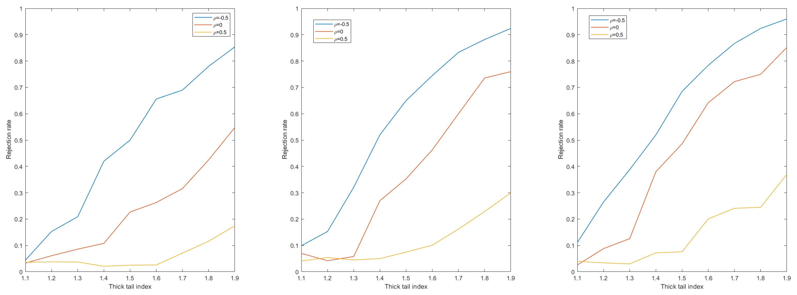
Comparing Figure 1, Figure 2, Figure 3 and Figure 4, it is not difficult to find that ${\mathrm{\Xi }}_1$ has a relatively stable empirical size and a high empirical power, but when the change point appears in the latter half of the observation sequence the empirical power is not satisfactory.

It is not difficult to find that the heavy-tailed index $\kappa$ is in the limit distribution. Although some scholars have proposed a series of methods to estimate $\kappa$ (see [21,22]), their effectiveness is not satisfactory. Therefore, in order to avoid estimating $\kappa$, we recommend using bootstrap sampling to approximate the limit distribution of the statistic under the null hypothesis, so as to obtain an accurate critical value. The specific steps are as follows:

Step 1. Use the regression of $X_t$ on the intercept to calculate the ordinary least squares (OLS) residual ${\hat{e}}_j$, and then calculate the OLS residual ${\hat{\eta }}_j$ from the regression of ${\hat{e}}_j$ on ${\hat{e}}_{j-1}$.

Step 2. Compute the centered residuals

$${\eta }_t^0={\hat{\eta }}_{t+1}-{(n-1)}^{-1}\sum _{j=2}^n{\hat{\eta }}_j,$$

$${\eta }_t^1={\hat{\eta }}_{t+1}-{(k-1)}^{-1}\sum _{j=2}^k{\hat{\eta }}_j,$$

and

$${\eta }_t^2={\hat{\eta }}_{t+1}-{(n-k-1)}^{-1}\sum _{j=k+2}^n{\hat{\eta }}_j.$$

Step 3. For a fixed number $m<n$, we extract bootstrap samples ${\check{\eta }}_2,\cdots ,{\check{\eta }}_m$ from ${\eta }_2^0$, ⋯, ${\eta }_n^0$, ${\tilde{\eta }}_2,\cdots ,{\tilde{\eta }}_{k^{\prime }}$ from ${\eta }_2^1$, ⋯, ${\eta }_k^1$, and ${\tilde{\eta }}_{k^{\prime }+2},\cdots ,{\tilde{\eta }}_m$ from ${\eta }_{k+2}^2$, ${\eta }_{k+3}^2$, ⋯, ${\eta }_n^1$.

Step 4. Constructing the bootstrap statistic:

$${\tilde{\mathrm{\Xi }}}_1^{*}=\underset{m{v}_1\le k^{\prime }\le m{v}_2}{\max }{\tilde{R}}_1\left(k^{\prime }\right),$$

$${\tilde{R}}_1\left(k^{\prime }\right)=\frac{\left|{\sum }_{j=2}^{k^{\prime }}({\check{\eta }}_j-{\overline{\check{\eta }}}_m)\right|}{m^{-1/2}{\left\{{\sum }_{i=2}^{k^{\prime }}{\left[{\sum }_{j=2}^i({\tilde{\eta }}_j-{\overline{\tilde{\eta }}}_{k^{\prime }})\right]}^2+{\sum }_{i=k^{\prime }+2}^m{\left[{\sum }_{j=k^{\prime }+2}^i({\tilde{\eta }}_j-{\widetilde{\stackrel{~}{\eta }}}_{k^{\prime }})\right]}^2\right\}}^{1/2}},$$

where ${\overline{\check{\eta }}}_m={(m-1)}^{-1}{\sum }_{j=2}^m{\check{\eta }}_j$, ${\overline{\tilde{\eta }}}_{k^{\prime }}={(k^{\prime }-1)}^{-1}{\sum }_{j=2}^{k^{\prime }}{\tilde{\eta }}_j$, and ${\widetilde{\stackrel{~}{\eta }}}_{k^{\prime }}={(m-k^{\prime }-1)}^{-1}{\sum }_{j=k^{\prime }+2}^m{\tilde{\eta }}_j$.

Step 5. Repeat steps 3 and 4 1000 times, then we obtain a set of statistics $\{{\tilde{\mathrm{\Xi }}}_1^{*1},\cdots ,{\tilde{\mathrm{\Xi }}}_1^{*1000}\}$.

Step 6. Calculate the $\alpha$-quantile ${\tilde{\mathrm{\Xi }}}_1^{*}\left(\alpha \right)$ of $\{{\tilde{\mathrm{\Xi }}}_1^{*1},\cdots ,{\tilde{\mathrm{\Xi }}}_1^{*1000}\}$. If ${\mathrm{\Xi }}_1>{\tilde{\mathrm{\Xi }}}_1^{*}\left(\alpha \right)$, then reject the null hypothesis.

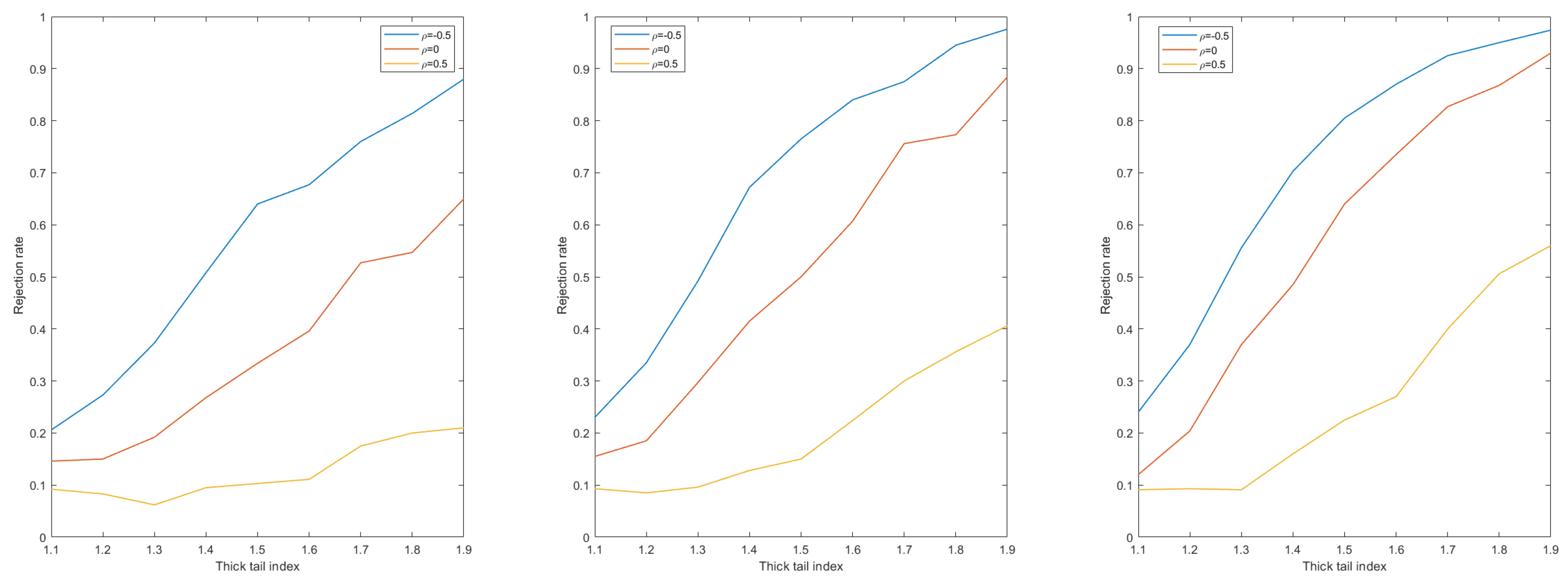
Remark 4.

Choosing a suitable m is very difficult, but Mcmurry et al. [23] provided an ideal choice for controlling the empirical power: $m=\left[\frac{4n}{\log n}\right]$. Therefore, it is necessary to use this numerical value for the simulation experiments.

As we guessed, Figure 5 shows a satisfactory result, especially for the case of $\rho =0.5$, where the increase in empirical power is significant, and this indicates that the position of the change point has a small impact on the newly constructed statistic.

To expand the comparison, the jackknife method is used, the steps of which are as follows.

Step 1. Use the regression of $X_t$ on the intercept to calculate the ordinary least squares (OLS) residual ${\hat{e}}_j$, and then calculate the OLS residual ${\hat{\eta }}_j$ from the regression of ${\hat{e}}_j$ on ${\hat{e}}_{j-1}$.

Step 2. Compute the centered residuals

$${\eta }_t^0={\hat{\eta }}_{t+1}-{(n-1)}^{-1}\sum _{j=2}^n{\hat{\eta }}_j,$$

$${\eta }_t^1={\hat{\eta }}_{t+1}-{(k-1)}^{-1}\sum _{j=2}^k{\hat{\eta }}_j,$$

and

$${\eta }_t^2={\hat{\eta }}_{t+1}-{(n-k-1)}^{-1}\sum _{j=k+2}^n{\hat{\eta }}_j.$$

Step 3. We extract jackknife samples ${\dot{\eta }}_2,\cdots ,{\dot{\eta }}_{n-1}$ from ${\eta }_2^0$, ⋯, ${\eta }_n^0$, ${\ddot{\eta }}_2,\cdots ,{\ddot{\eta }}_{k-1}$ from ${\eta }_2^1$, ⋯, ${\eta }_k^1$, and ${\stackrel{...}{\eta }}_{k+2},\cdots ,{\stackrel{...}{\eta }}_{n-1}$ from ${\eta }_{k+2}^2$, ${\eta }_{k+3}^2$, ⋯, ${\eta }_n^2$.

Step 4. Constructing the jackknife statistic:

$${\tilde{\mathrm{\Xi }}}_2=\underset{n{v}_1\le k\le n{v}_2}{\max }{R}_2,$$

$$R_2=\frac{\left|{\sum }_{j=2}^k({\dot{\eta }}_j-{\overline{\dot{\eta }}}_{n-1})\right|}{n^{-1/2}{\left\{{\sum }_{i=2}^k{\left[{\sum }_{j=2}^i({\ddot{\eta }}_j-{\overline{\ddot{\eta }}}_k)\right]}^2+{\sum }_{i=k+2}^{n-1}{\left[{\sum }_{j=k+2}^i({\stackrel{...}{\eta }}_j-{\overline{\stackrel{...}{\eta }}}_k)\right]}^2\right\}}^{1/2}},$$

where ${\overline{\dot{\eta }}}_{n-1}={(n-2)}^{-1}{\sum }_{j=2}^{n-1}{\dot{\eta }}_j$, ${\overline{\ddot{\eta }}}_k={(k-2)}^{-1}{\sum }_{j=2}^k{\ddot{\eta }}_j$, and ${\overline{\stackrel{...}{\eta }}}_k={(n-k-2)}^{-1}{\sum }_{j=k+2}^{n-1}{\stackrel{...}{\eta }}_j$.

Step 5. Repeat steps 3 and 4 1000 times, then we obtain a set of statistics $\{{\tilde{\mathrm{\Xi }}}_2^1,\cdots ,{\tilde{\mathrm{\Xi }}}_2^{1000}\}$.

Step 6. Calculate the $\alpha$-quantile ${\tilde{\mathrm{\Xi }}}_2\left(\alpha \right)$ of $\{{\tilde{\mathrm{\Xi }}}_2^1,\cdots ,{\tilde{\mathrm{\Xi }}}_2^{1000}\}$. If ${\mathrm{\Xi }}_1>{\tilde{\mathrm{\Xi }}}_2\left(\alpha \right)$, then reject the null hypothesis.

Similarly, the power of the jackknife statistic can be obtained as shown in Figure 6.

As a classical sampling method, the limiting distribution of a statistic under the null hypothesis can also be approximated using the subsampling method to obtain more accurate critical values and power, as follows:

Step 1. Use the regression of $X_t$ on the intercept to calculate the ordinary least squares (OLS) residual ${\hat{e}}_j$, and then calculate the OLS residual ${\hat{\eta }}_j$ from the regression of ${\hat{e}}_j$ on ${\hat{e}}_{j-1}$.

Step 2. Compute the centered residuals ${\eta }_t^0={\hat{\eta }}_{t+1}-{(n-1)}^{-1}{\sum }_{j=2}^n{\hat{\eta }}_j$.

Step 3. For a fixed number $b<n$, we extract $n-1-b$ processes with length b, and satisfy the null hypothesis. For $l=1,2,\cdots ,n-1-b$, the l-th process is determined by ${\eta }_l^0,{\eta }_{l+1}^0,\cdots ,{\eta }_{l+b-1}^0$.

Step 4. We extract ${\mathrm{\Xi }}_{b,l}$ based on ${\eta }_l^0,{\eta }_{l+1}^0,\cdots ,{\eta }_{l+b-1}^0$:

$${\mathrm{\Xi }}_{b,l}=\underset{0\le v\le 1}{\max }{R}_3,$$

$$\begin{array}{cc}\hfill & R_3=\hfill \\ \hfill & \frac{b^{1/2}\left|{\sum }_{j=l}^{l+(b-1)v}({\eta }_j^0-{\overline{\eta }}_{l,l+b-1}^0)\right|}{{\left\{{\sum }_{i=l}^{l+(b-1)v}{\left[{\sum }_{j=l}^i({\eta }_j^0-{\overline{\eta }}_{l,l+(b-1)v}^0)\right]}^2+{\sum }_{i=l+(b-1)v+1}^{l+b-1}{\left[{\sum }_{j=l+(b-1)v+1}^i({\eta }_j^0-{\overline{\eta }}_{l+(b-1)v,l+b-1})\right]}^2\right\}}^{1/2}},\hfill \end{array}$$

where ${\overline{\eta }}_{m,n}^0={(n-m-1)}^{-1}{\sum }_{j=m}^n{\eta }_j^0$.

Step 5. ${\mathrm{\Xi }}_b\left(\alpha \right)$ is the $\alpha$-quantile of the empirical distributions of the $n-b-1$ value ${\mathrm{\Xi }}_{b,l}$. When ${\mathrm{\Xi }}_1>{\mathrm{\Xi }}_b\left(\alpha \right)$, we reject the null hypothesis.

Combining Figure 5, Figure 6 and Figure 7, it can be seen that there is a large increase in the power by reconstructing the bootstrap statistic, the jackknife statistic, and the subsampling statistic from the original. Combining the comparisons it is easy to see that the bootstrap method has the most significant effect on the increase in power and the jackknife method has the least effect. The reason for this may be because bootstrap sampling is a nonparametric statistical method, the basic idea of which is to obtain more reliable estimates of the statistical properties of the original sample by drawing a large number of subsamples from the original sample and then making statistical inferences on these subsamples. Since the original series may contain extreme values, these extreme values may have an impact on the statistical inference. The bootstrap sampling method is effective in reducing the impact of extreme values, which may occur less frequently when subsamples are drawn.

Since jackknife sampling excludes only one observation per iteration, it may not be effective in reducing the impact of extreme values or “heavy tails” for data with these points. In contrast, bootstrap sampling can better simulate the distribution of the original data by generating a number of random subsets of the original data size (via put-back sampling), especially for non-normally distributed data. The bootstrap method can be applied to any form of statistic, giving it greater flexibility in dealing with more complex statistical problems.

5. Application

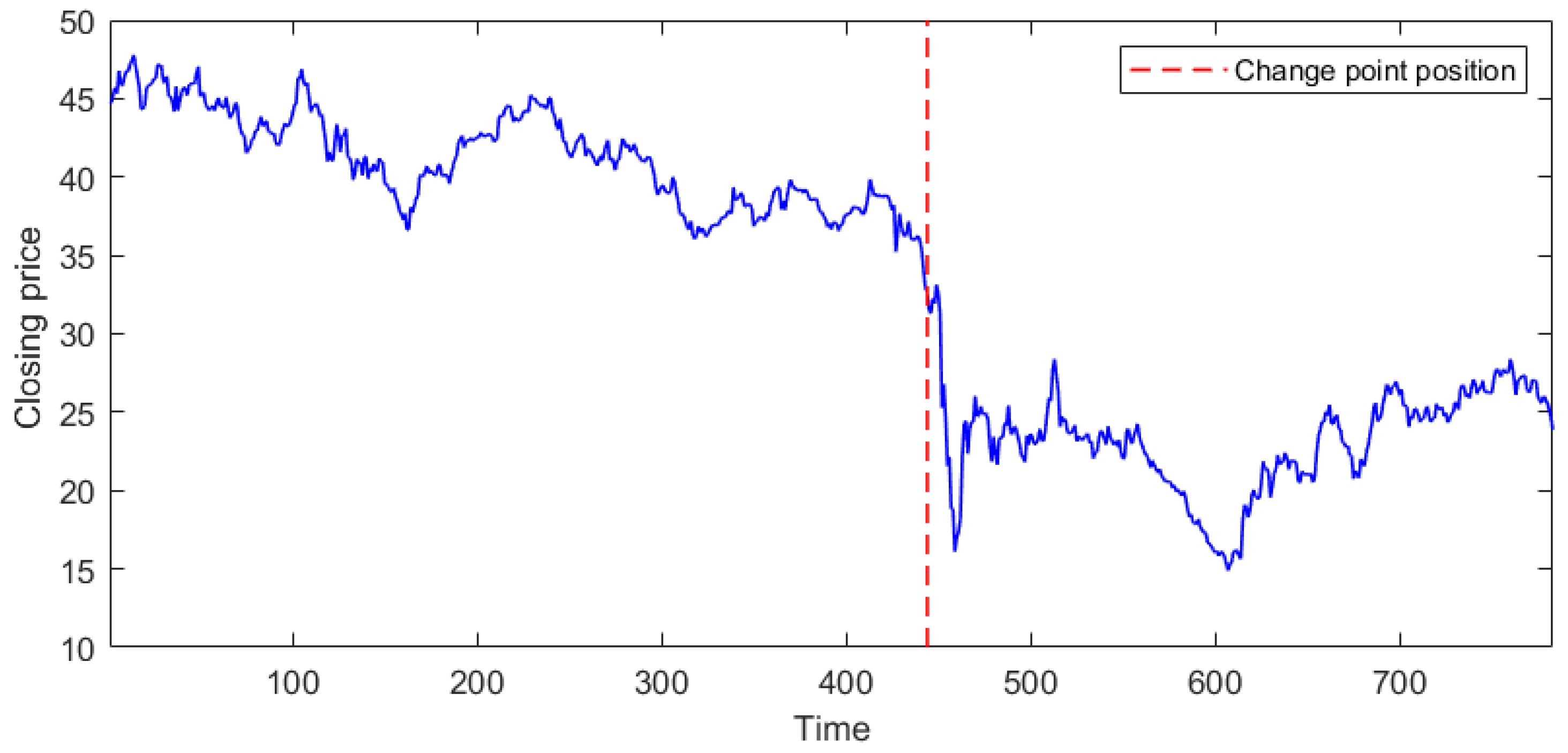
We consider the closing price data of British Petroleum (BP) between February 2019 and July 2021 (783 observations). Upon observation, it is easy to see that there seems to be a point of mean change in this sequence of observations, but it is unscientific to rely on visual perception alone. Therefore, the test statistic needs to be utilized to verify that it has a change point.

According to the description in the previous section, the bootstrap method has the best performance, so we consider using the bootstrap method for this problem.

Based on John [24], Jin, et al. [13] believe that the data can be fitted as a heavy-tailed sequence with a tailed index $\kappa =1.732$. Under the premise that the process has infinite variance, we use the ARMA model to fit a causal AR model, and using the Bayesian information criterion, the sample partial autocorrelation function of the AR(1) model is almost zero after a first-order lag, and its autoregressive coefficient is 0.5788. Jin, et al. [25] proposed a mean change point estimator based on a heavy-tailed sequence and proved the consistency of the estimator. Based on this, we obtain the change position $k^{*}=444$ (see Figure 8). Then, the entire sequence is divided into two parts (1,444) and (445,783), with mean values ${\hat{\mu }}_1=41.23$ and ${\hat{\mu }}_2=23.34$, respectively. A mean-corrected sequence is based on ${\mu }_t$, where ${\mu }_t=X_t-{\hat{\mu }}_1$, $t=1,\cdots ,444$, ${\mu }_t=X_t-{\hat{\mu }}_2$, $t=445,\cdots ,783$. It is not difficult to find that the heavy-tailed character of the original data has not changed in the corrected sequence.

For the statistic ${\mathrm{\Xi }}_1$, we obtain a critical value of 5.9551 (see

Table 1. A series of values related to the BP closing price.

$\kappa$	$k^{*}$	Critical value of ${\mathrm{\Xi }}_1$	${\mathrm{\Xi }}_1$	Critical value of ${\tilde{\mathrm{\Xi }}}_1^{*}$
1.732	444	5.9551	5.4446	3.0627

), and the critical value 3.0627 based on bootstrap testing. By replacing with the original data, ${\mathrm{\Xi }}_1=5.4446$ can be obtained. As we guessed, ${\mathrm{\Xi }}_1$ is greater than the critical value obtained based on the bootstrap method, we reject the null hypothesis and believe that there is a change point. But ${\mathrm{\Xi }}_1<5.9951$, that is, in the case of the original statistic, we cannot consider the sequence to have a change point, so this also reflects the superiority of the bootstrap method. Therefore, this is sufficient to demonstrate the good performance of our proposed method.

6. Conclusions

This paper proposes a modified ratio test based on a heavy-tailed AR(p) model, we obtain that the asymptotic distributions of these modified statistics are functionals of Lévy processes and that there are consistencies under the alternative hypothesis. These sampling methods provide more asymptotically accurate critical values, making the final simulation results show that the ratio test based on these sampling methods have good empirical power. Meanwhile, we consider the closing price of BP, further highlighting the rationality and superiority of our proposed methods.

The disadvantages of the statistic are obvious. For example, the performance of our statistics when the position of the change point is behind is actually not satisfactory enough. Moreover, if there are multiple change points in the sequence, our statistics may not be applicable. Future research work should not only focus on the issues of mean changes, but also consider more possible situations.

References

1. Pepelyshev, A.; Polunchenko, A. Real-time financial surveillance via quickest change-point detection methods. Stat. Interface 2017, 10, 93–106. [Google Scholar] [CrossRef]
2. Ghosh, P.; Vaida, F. Random change point modelling of HIV immunologic responses. Stat. Med. 2007, 26, 2074–2087. [Google Scholar] [CrossRef] [PubMed]
3. Punt, A.E.; Szuwalski, C.S.; Stockhausen, W. An evaluation of stock-recruitment proxies and environmental change points for implementing the US Sustainable Fisheries Act. Fish Res. 2014, 157, 28–40. [Google Scholar] [CrossRef]
4. Csörgo, M.; Horváth, L. Limit Theorems in Change-Point Analysis; John Wiley & Sons: Hoboken, NJ, USA, 1997. [Google Scholar]
5. Horváth, L.; Hušková, M. Change-point detection in panel data. J. Time Ser. Anal. 2012, 33, 631–648. [Google Scholar] [CrossRef]
6. Horváth, L.; Rice, G. Extensions of some classical methods in change point analysis. Test-Spain 2014, 23, 219–255. [Google Scholar] [CrossRef]
7. Gao, M.; Ding, S.S.; Wu, S.P.; Yang, W. The asymptotic distribution of CUSUM estimator based on α-mixing sequences. Commun. Stat.-Simul. Comput. 2020, 51, 6101–6113. [Google Scholar] [CrossRef]
8. Ding, S.; Fang, H.; Dong, X.; Yang, W. The CUSUM statistics of change-point models based on dependent sequences. J. Appl. Stat. 2021, 49, 2593–2611. [Google Scholar] [CrossRef]
9. Xu, M.; Wu, Y.; Jin, B. Detection of a change-point in variance by a weighted sum of powers of variances test. J. Appl. Stat. 2019, 46, 664–679. [Google Scholar] [CrossRef]
10. Guillaume, D.M.; Dacorogna, M.M.; Davé, R.R.; Müller, U.A.; Olsen, R.B.; Pictet, O.V. From the bird’s eye to the microscope: A survey of new stylized facts of the intra-daily foreign exchange markets. Financ Stoch. 1997, 1, 95–129. [Google Scholar] [CrossRef]
11. Mittnik, S.; Rachev, S. Stable Paretian Models in Finance; Wiley: New York, NY, USA, 2000. [Google Scholar]
12. Qin, R.B.; Yang, X.Q.; Chen, Z.S. Ratio detections for change point in heavy tailed observations. Commun. Stat.-Simul. Comput. 2019, 51, 2487–2510. [Google Scholar] [CrossRef]
13. Jin, H.; Wang, A.; Zhang, S.; Liu, J. Subsampling ratio tests for structural changes in time series with heavy-tailed AR(p) errors. Commun. Stat.-Simul. Comput. 2022, 1–27. [Google Scholar] [CrossRef]
14. Aue, A.; Horváth, L. Structural breaks in time series. J. Time Ser. Anal. 2013, 34, 1–16. [Google Scholar] [CrossRef]
15. Moon, J.; Hossain, M.B.; Chon, K.H. AR and ARMA model order selection for time-series modeling with ImageNet classification. Signal Process. 2021, 183, 108026. [Google Scholar] [CrossRef]
16. Jiang, H.; Duan, S.; Huang, L.; Han, Y.; Yang, H.; Ma, Q. Scale effects in AR model real-time ship motion prediction. Ocean Eng. 2020, 203, 107202. [Google Scholar] [CrossRef]
17. Movahed, T.M.; Bidgoly, H.J.; Manesh, M.H.K.; Mirzaei, H.R. Predicting cancer cells progression via entropy generation based on AR and ARMA models. Int. Commun. Heat Mass. 2021, 127, 105565. [Google Scholar] [CrossRef]
18. Kokoszka, P.; Wolf, M. Subsampling the mean of heavy-tailed dependent observations. J. Time Ser. Anal. 2004, 32, 217–234. [Google Scholar] [CrossRef]
19. Shao, X.F. A simple test of changes in mean in the possible presence of long-range dependence. J. Time Ser. Anal. 2011, 32, 598–606. [Google Scholar] [CrossRef]
20. Phillips, P.C.B.; Solo, V. Asymptotics for linear processes. Ann. Stat. 1992, 20, 971–1001. [Google Scholar] [CrossRef]
21. Koedijk, K.; Schafgans, M.; de Vries, C. The tail index of exchange rate returns. J. Int. Econ. 1990, 29, 93–108. [Google Scholar] [CrossRef]
22. Resnick, S.I. Heavy-Tail Phenomena Probabilistic and Statistical Modeling; Springer: New York, NY, USA, 2007. [Google Scholar]
23. Mcmurry, T.L.; Politis, D.N. Banded and tapered estimates for autocovariance matrices and the linear process bootstrap. J. Time Ser. Anal. 2010, 31, 471–482. [Google Scholar] [CrossRef]
24. John, P.N. Numerical calculation of stable densities and distribution functions. Commun. Stat. Stoch. Models 1997, 13, 759–774. [Google Scholar]
25. Jin, H.; Tian, Z.; Qin, R.B. Bootstrap tests for structural change with infinite variance observation. Stat. Probab. Lett. 2009, 79, 1985–1995. [Google Scholar] [CrossRef]
Figure 1. Empirical sizes of Ξ 1 with n = 200 , 500 , 800 .
Mathematics 11 03988 g001
Figure 2. Empirical power of Ξ 1 with Δ 1 = 2 , k * = 0.3 n , and n = 200 , 500 , 800 .
Mathematics 11 03988 g002
Figure 3. Empirical power of Ξ 1 with Δ 1 = 4 , k * = 0.3 n , and n = 200 , 500 , 800 .
Mathematics 11 03988 g003
Figure 4. Empirical power of Ξ 1 with Δ 1 = 2 , k * = 0.7 n , and n = 200 , 500 , 800 .
Mathematics 11 03988 g004
Figure 5. Empirical power of Ξ ~ 1 * with Δ 1 = 2 , k * = 0.7 n , and n = 200 , 500 , 800 .
Mathematics 11 03988 g005
Figure 6. Empirical power of Ξ ~ 2 with Δ 1 = 2 , k * = 0.7 n , and n = 200 , 500 , 800 .
Mathematics 11 03988 g006
Figure 7. Empirical power of Ξ b , l with Δ 1 = 2 , k * = 0.7 n , and n = 200 , 500 , 800 .
Mathematics 11 03988 g007
Figure 8. Closing price of BP.
Mathematics 11 03988 g008