Article

Epidemic Waves in a Stochastic SIRVI Epidemic Model Incorporating the Ornstein–Uhlenbeck Process

by
Fehaid Salem Alshammari
* and
Fahir Talay Akyildiz
Department of Mathematics and Statistics, Faculty of Science, Imam Mohammad Ibn Saud Islamic University (IMSIU), Riyadh 11432, Saudi Arabia
*
Author to whom correspondence should be addressed.
Mathematics 2023, 11(18), 3876; https://doi.org/10.3390/math11183876
Submission received: 10 July 2023 / Revised: 5 September 2023 / Accepted: 9 September 2023 / Published: 11 September 2023
(This article belongs to the Special Issue Stochastic Dynamics in Computational and Mathematical Biology)

Abstract

:
The worldwide data for COVID-19 for active, infected individuals in multiple waves show that traditional epidemic models with constant parameters are not able to capture this kind of disease behavior. We solved this major open mathematical problem in this report. We first consider the disease transmission rate for the stochastic SIRVI epidemic model, which satisfies the mean-reverting Ornstein–Uhlenbeck (OU) process, and we propose a new stochastic SIRVI model. We then showed the existence and uniqueness of the global solution and obtained sufficient conditions for the persistent mean and exponential extinction of infectious disease, which have not been given before. In the second part, we derive a nonlinear system of differential equations for the time-dependent transmission rate from the deterministic SIRVI model and present an algorithm to compute the time-dependent transmission rate directly from the given active, infected individuals’ data. We then show that the time-dependent transmission obtained from and perturbed by the Ornstein–Uhlenbeck process could be represented after using a smoothing technique using a finite linear combination of a Gaussian radial basis function, which was obtained from our algorithm. This novel computer-assisted proof provides a theoretical basis for other epidemic models and epidemic waves. Finally, some numerical solutions of the stochastic SIRVI model are presented using COVID-19 data from Saudi Arabia and Austria.

1. Introduction

The aim of epidemic dynamics is to build up a mathematical model that can reflect the biological mechanism according to development, occurrence, variance, and the effect of environmental factors on diseases. In 1760, Daniel Bernoulli developed the first mathematical model to explore the transmission of an infectious disease, which was smallpox. Then, numerous mathematical models were developed to study the transmission dynamics of different diseases, aiming to predict, assess, and control their transmission [1,2,3,4]. One of the simplest models is the standard susceptible-infected-recovered (SIR) model, which was originally proposed by Kermack and McKendrick in a series of three papers [5,6,7]. Recent variations on the SIR mathematical model take into consideration physiological, social, and economic demands [8]. It is well known that infectious diseases pose a great threat to human life. Therefore, the prevention and strong control of infectious diseases is very crucial. Vaccination programs may help control the transmission of many diseases [9]; hence, the term vaccination must be included in epidemic modeling. The susceptible-infected-recovered-vaccination (SIRV) model in [10,11,12,13] and the susceptible-infected-recovered-vaccination-death (SIRVD) model [14] study the effect of vaccination on disease transmission worldwide. Omae et al. studied the effect of first and second doses of vaccination on the transmission of COVID-19 [15]; they proposed the SIRVVD model and concluded that appropriate vaccination measures would sufficiently reduce the number of infected individuals and reduce the mortality rate. However, it is well known that there is still a possibility of getting infected after vaccination, and this is not considered in the reports mentioned above. Nevertheless, it is necessary to investigate the impact of vaccination in the case of temporal/weak immunity on disease transmission, as in SIRV epidemic models (see [16,17,18]). More recently, Turkyilmazoglu [19] considered the following SIRVI epidemic model with temporal/weak immunity, as is shown in Figure 1. If we consider the same system with recruitment rate ( Λ ) and natural date rate ( μ ) , then the system of ordinary differential equations in [19] becomes
d S d t = Λ β ^ S I ν S μ S ,   S ( t = 0 ) = S 0 d I d t = β ^ S I + α V I γ I μ I ,   I ( t = 0 ) = I 0 d V d t = ν S α V I μ V ,   V ( t = 0 ) = V 0 d R d t = γ I μ R ,   R ( t = 0 ) = R 0 = 0 }  
where β ^ represents the transmission rate of disease to the susceptible population, α is the transmission rate between vaccinees and infected individuals, ν is the vaccination rate, and γ denotes recovery rate. All parameters here are positive. Since R ( t ) is not involved in the first three equations, we can consider the last equation separately.
However, in the real world, different forms of random factors affect disease transmission and some of the biological parameters, such as disease transmission rate and per capita birth rate and mortality. In order to study the dynamic properties of an ecosystem with a changing environment, scientists generally consider that the basic parameters of a model are affected by environmental noise. Regarding stochastic biological mathematical models, there are basically two methods to randomize the model parameters in a random environment; one of them is Gaussian linear white noise, which was assimilated in many papers to adopt environmental variability in the parameters, for example [20,21,22,23,24].
However, as pointed out by E Allen in [25], the mean-reverting processes possess several important features that better characterize environmental variability in biological systems when compared with the linear function of white noise; more importantly, he stated that mean-reverting processes are conceptually and biologically realistic when compared to the linear function of white noise. Therefore, many authors assimilated the Ornstein–Uhlenbeck process for the parameters in a random environment. For example, Y Song and X Zhang, in [26], considered a stochastic SVEIS epidemic model, incorporating the Ornstein–Uhlenbeck process, and they proved that this stochastic model has a stationary distribution when the critical value of the stochastic reproducing number is greater than one. They also established sufficient conditions on the stochastic reproducing number for exponential extinction. This study is different from our study; we consider transmission rate by initially satisfying the mean reverting OU process, and we then show that the transmission rate can be written as a finite linear combination of a Gaussian radial basis function ( β ( t ) s 0 + n = 1 N s n ϕ ( ε ( t ζ n ) ) ,   ϕ ( r ) = e ( ε r ) 2 ) . Because of this reason, in our study, β ^ is the most important parameter, which is in a randomly varying environment, where we assume, initially, that the disease transmission rate, β ^ , satisfies the mean reverting OU process.
β = r ( β ^ β ( t ) ) d t + σ d B  
where r > 0 is the speed of reversion, σ is the intensity of volatility, and B ( t ) is the standard Brownian motion; Equation (2) can be solved easily as
β ( t ) = β ^ + e r t ( β ^ + β ( 0 ) + 0 t σ e r z d B ( z ) )  
The average disease transmission rate β ¯ on any time interval [ 0 , T ] is found to be
β ¯ = 1 T 0 T β ( t ) d t = β ^ + 1 T 0 T σ r ( 1 e r ( s T ) ) d B ( s ) ~ ( β ^ ,   σ 2 T 3 + O ( T 2 ) )
so that 𝔼 ( β ¯ ) = β ^ and 𝕍ar ( β ¯ ) = σ 2 T 3 + O ( T 2 ) [27]. The variance in the average disease transmission rate tends to zero as T 0 . If we now assume that Gaussian linear white noise perturbs the transmission rate in model (1), then we have
β ( t ) = β ^ + σ d B d t  
For any time interval [ 0 , T ] , the average value is
β ¯ = 1 T 0 T β ( t ) d t = β ^ + B ( T ) T ~ N ( β , ¯ σ 2 T )  
Clearly, E ( β ¯ ) = β ^ and Var ( β ¯ ) = σ 2 T . It is not difficult to see that Var ( β ¯ ) as the time interval T 0 . Hence, it is more acceptable to introduce the OU process to perturb the parameters in the epidemic model than Gaussian linear white noise. Based on the above conclusion, let us replace β ¯ with the OU process β ( t ) in system (1)a–c and consider incorporating the OU process; thus, from (1)a–c, we obtain
d S = ( Λ β + ( t ) S I ν S μ S ) d t ,   d I = ( β + ( t ) S I + α V I γ I μ I ) d t d V = ( ν S α V I μ V ) d t , d β ( t ) = r ( β ^ β ( t ) ) + σ d B ( t ) }  
where β + ( t ) = max { β ( t ) , 0 } . By adding the first three equations in (7) and solving the result, we have S ( t ) + I ( t ) + V ( t ) A μ + [ S ( 0 ) + I ( 0 ) + V ( 0 ) A μ ] e μ t . If we assume that S ( 0 ) + I ( 0 ) + V ( 0 ) A μ , then we can define the set by Ξ = { ( S ( t ) , I ( t ) , V ( t ) ,   β ( t ) ) + 3 × :   S ( t ) + I ( t ) + V ( t ) A μ } , which is the invariant set of system (7).
This article is organized as follows: the existence and uniqueness of the positive solution of system (7) are shown in Section 2. In this section, we also develop a suitable Lyapunov function and use the method of Khasminskii [28] to show the existence of a stationary distribution of solutions in terms of model (7). In Section 3, we assume the transmission rate in system (1) to be time-dependent, derive a nonlinear differential equation, and present an algorithm and numerical solutions for the time-dependent transmission rate directly from COVID-19 data from Saudi Arabia. In Section 4, we numerically solve the transmission rate perturbed from the OU process and compare the result with the prediction obtained from our algorithm. An exponential smoothing technique is used for the transmission rate obtained from the OU process, and the numerical solutions of the system in Equation (7) are also given in this section. The last section is devoted to the conclusion of the present results.

2. Existence of the Unique Global Positive Solution

Theorem 1. 
Given any initial value  ( S ( 0 ) , I ( 0 ) , V ( 0 ) ,   β ( 0 ) ) Ξ , system (7) has a unique solution:   ( S ( t ) , I ( t ) , V ( t ) ,   β ( t ) ) ,   t > 0 . Furthermore, the solution will remain in  + 3 ×  with a probability equal to 1.
Proof. 
Constructing the C 2 -function V 0 on + 3 as
V 0 = ( S C C ln S C ) + ( I 1 ln I ) + ( V 1 ln V ) + C 1 x ( t ) 2  
where C and C 1 are the constants to be defined later, and x ( t ) = β + ( t ) β ^ when applying It o ^ ’s formula; the action of differential operator L on V 0 is
L V 0 = Λ μ S C ( Λ S + ( x ( t ) + β ^ ) I + υ + μ ) γ I μ I β + S α V + γ + 2 μ μ V υ S V + α I C 1 r x 2 ( t )   Λ + C ( μ + υ ) + γ + 2 μ + C Λ μ ( | x | x 2 ( t ) )   K ¯
where C = γ α + μ β + , C 1 = C Λ μ , and K ¯ is a positive constant, which is independent of the initial condition. For the rest of the proof, it has exactly the same line as in [27]; hence, it is omitted here. This completes the proof. □
Theorem 2. 
Assume that
R 0 s = β ^ Λ ( ν + μ + Λ μ σ 2 π r ) ( γ + μ ) + α ν μ ( ν + μ + Λ μ σ 2 π r ) ( γ + μ ) > 1  
and  lim t inf V 1 ( t ) t 0   ( V 1 = ( b 1 + b 5 ) ln S ln I b 3 ln V + b 2 S + ( S + I + V ) b 4 ) . Then, for any initial value,  Z ( 0 ) = ( S ( 0 ) ,   I ( 0 ) , R ( 0 ) )   Ω , the solution of (7) has the following:
lim t inf 1 t 0 t I d τ ( γ + μ ) ( α b 3 + b b 1 + b 1 b 5 )   ( R 0 s 1 )  
where
b 2 = β ^ Λ ( ν + μ + Λ μ σ 2 π r ) ,   b 1 = b 2 ( ν + μ + Λ μ σ 2 π r ) ,   b 3 = α η b 2 β + μ 2 ,   b 4 = μ b 3 , b 5 = α η b 1 μ
Proof. 
We define a series of Lyapunov functions. Define V 1 = ( b 1 + b 5 ) ln S ln I b 3 ln V + b 2 S + ( S + I + V ) b 4 . By applying Itô’s formula, we obtain
L V 1 = L b 1 + b 5 ln S ln I b 3 ln V + b 2 S + S + I + V b 4 = I β + t Λ S + ν + μ b 1 + b 5 α V S β + t + γ + μ + ν S V + α I + μ b 3 + Λ I S β + t ν + μ S b 2 + Λ μ S + I + V γ b 4 f 3 Λ β + t b 1 b 2 3 4 Λ η α b 3 b 4 b 5 4 + b 1 ν + μ + Λ μ σ 2 π r + b 1 x t b 1 max x t , 0 θ τ d τ + b 2 + b 3 μ + b 1 ν + μ + Λ μ σ 2 π r + b 5 x t b 5 max x t , 0 θ τ d τ + α b 3 + β + b 1 + b 1 b 5 I + γ + μ
As before, assume that
b 2 = β ^ Λ ( ν + μ + Λ μ σ 2 π r ) ,   b 1 = b 2 ( ν + μ + Λ μ σ 2 π r ) ,   b 3 = α η b 2 β + μ 2 ,   b 4 = μ b 3 , b 5 = α η b 1 μ  
then,
V 1 ( γ + μ ) ( R 0 s 1 ) + | x ( t ) | ( b 1 + b 5 ) + ( α b 3 + β + b 1 + b 1 b 5 ) I + 3 b b 1 b 2 3 3 A β + ( t ) b 1 b 2 3 + b 1 max { x ( t ) , 0 } θ ( τ ) d τ b 1 max { x ( t ) , 0 } θ ( τ ) d τ  
where
R 0 s = β ^ Λ ( ν + μ + Λ μ σ 2 π r ) ( γ + μ ) + α Λ ν μ ( ν + μ + Λ μ σ 2 π r ) ( γ + μ )
and from [22], we have
lim t 1 t E [ 1 t 0 t max { x ( τ ) , 0 } d τ max { x ( τ ) , 0 } θ ( τ ) d τ ] = E [ 0 x ( τ ) θ ( τ ) d τ   ] 0 x ( τ ) θ ( τ ) d τ = 0
lim t inf 1 t 0 t ( α b 3 + β + b 1 + b 1 b 5 ) I d τ ( γ + μ )   ( R 0 s 1 ) + lim t inf V 1 ( t ) V 1 ( 0 ) t  
Since we assume lim t inf V 1 ( t ) t 0 . Then, we obtain
lim t inf 1 t 0 t I d τ ( γ + μ ) ( α b 3 + β + b 1 + b 1 b 5 )   ( R 0 s 1 )  
In other words, the disease will spread in the world. □
Theorem 3. 
If  μ + ν < 1   a n d   R 0 e = b Λ ( 1 + α ) + σ 2 π r μ ( ν + μ ) ( γ + μ ) < 1 ,  then the disease of system (7) will tend to zero exponentially with a probability of one.
Proof. 
When applying the generalized Itô’s formula,
V 4 = ln I + 1 ν μ μ ( ν + μ )   ln I  
and we have,
d ( V 4 ) = ( ( β ^ + x ( t ) ) S + α V ) ( γ + μ ) ( β ^ + x ( t ) ) Λ μ + α Λ μ ( γ + μ ) + 1 ν μ μ ( ν + μ ) ( ( β ^ + x ( t ) ) Λ μ + α Λ μ ) = β ^ Λ μ ( ν + μ ) + α β ^ Λ μ ( ν + μ ) ( γ + μ ) + | x ( t ) | Λ μ ( ν + μ )
By integrating (19) from zero to t and dividing by t, we obtain
V 4 ( t ) V 4 ( 0 ) t β ^ A ( 1 + α ) μ ( ν + μ ) ( γ + μ ) + Λ μ ( ν + μ ) 1 t 0 t | x ( τ ) | d τ  
By taking the superior limit on both sides of (17) and combining it with (12), we obtain
lim t sup V 4 ( t ) V 4 ( 0 ) t = ( γ + μ ) ( R 0 e 1 ) ,   a . s ,  
From here, we have
lim t sup ln I + 1 ν μ μ ( ν + μ )   ln I < 1 ,  
This shows that the disease I will tend to zero exponentially with a probability of one. This completes the proof. □

3. Driving Transmission Rate from the Infected Population for the Deterministic SIRVI Model and Numerical Solution

From Equation (1), we assume that the transmission rate is time-dependent. By solving S ( t ) from the second equation in (1) and substituting it into the first, we obtain
M ( I ( t ) ) d β 1 ( t ) d t + N ( I ( t ) ) β 1 2 ( t ) + P ( I ( t ) ) β 1 ( t ) = 0 .
where
M ( I ( t ) ) = I ( t ) ( ( γ + μ ) I ( t ) α V ( t ) I ( t ) + d I d t ) ,   N ( I ( t ) ) = I ( t ) M ( I ( t ) ) + Λ I 3 ( t ) ,
P ( I ( t ) ) = I 2 ( t ) ( ( α μ + α ν ) V ( t ) γ μ γ ν + α d V d t μ ( μ + ν ) ) ( μ + ν ) I ( t ) d I d t + ( d I d t ) 2 + I ( t ) d I d t I ( t ) d 2 I d t 2
If there is no vaccination, (23) is reduced to a differential equation, which is obtained from the classical SIR model with a time-dependent transmission rate [29]. In the case of vaccination, (23) must be coupled with the third equation in Equation (1). Since the analytical solution is not possible, we need a numerical method to solve Equations (23) and third equation of system (1); here, we used a finite difference technique. We now try to compute a grid function consisting of the values B 1 ,   B 2 , ,   B m , where B i is our approximation of the solution β 1 ( t i ) ; here, t i = i h   and h = t i + 1 t i are the step sizes, and we use centered, finite difference to approximate d I ( t ) d t , d 2 I ( t ) d t 2 , and d β ( t ) d t , if we replace d I ( t ) d t , d 2 I ( t ) d t 2 , and d β ( t ) d t by centered finite difference approximation.
D i j = i j + 1 i j 1 2 h ,   D 2 y j = i j + 1 2 i j + i j 1 h 2 , D B j = B j + 1 B j 1 2 h
we then obtain
M ( i ( t ) ) B j + 1 B j 1 2 h + N ( i ( t ) ) B j + 1 B j 1 + P ( I ( t ) ) B j 1 = 0 .
and similarly,
v j + 1 v j 1 2 h = ν s j 1 α v j 1 i j 1 μ v j 1  
where s j 1 = γ i j 1 + μ i j 1 α v j 1 i j 1 + i j + 1 i j 1 2 h B j 1 i j 1 .
We use the data provided by the Ministry of Health Saudi Arabia for the daily infected cases. Mathematically, there are infinitely many choices of B ( 0 ) , so we used some well-known values [30]. We will give the numerical solutions of (24) with (25) in the following section.

4. Numerical Simulations

In this section, in order to verify the theoretical results obtained in this article, the number of confirmed, recovered, and death cases in Saudi Arabia and Austria were used. They can be found on this website: https://ourworldindata.org/coronavirus/country (accessed on 5 June 2023). A graph of the daily active cases is given in Figure 2a,b. We note that vaccination started on 18 December 2020 in Saudi Arabia. In order to provide numerical simulations, we must first determine the value of the parameters. The birth rate for Saudi Arabia in 2020 was 17.097 births for 1000 people, and the death rate was 3.557. The Saudi Arabian population in 2020 was 34,813,871; hence, Λ S = n × N 365 = 1630 ,   μ S = 3.557 365 × 1000 = 9.7452 × 10 6 . For Austria, the birth rate, death rate, and population in 2020 are 9.939, 10.3, and 8,907,777, respectively; hence, Λ A = n × N 365 = 242.55 ,   μ A = 10.3 365 × 1000 = 2.8219 × 10 5 . We first give the numerical solutions from Equation (23) for the time-dependent transmission rate, whereby we first used the real data from the Ministry of Health in Saudi Arabia (Figure 3a). We see that the transmission rate initially increases with time, then reaches a peak at around day 50, and then fluctuates while decreasing. We can see some peak times, which is when we believe the government eased some of the restrictions, resulting in an increase in the value of the transmission rate that then reduces because people become more careful. In Figure 3b, we considered the transmission rate for the COVID-19 data of Austria, which was provided by the Ministry of Health in Austria. We can clearly see that the initial transmission rate was higher; it then oscillates, having four peaks. It is clear that both numerically obtained transmission rates can be approximated by finite linear combination using Gaussian radial basis functions. We note that if the infected population was a constant, then the transmission rate is zero, provided that μ = Λ = 0   ( constant   population ) . If there is a change in a country’s population, the transmission rate can be given by the following simple analytical function:
β ( t ) = μ ( γ + μ ) e μ t ( I C γ + I C μ Λ ) e μ t μ β ( 0 ) ( γ + μ )
where I C represents the constant of the infected individuals in the current day. Overall, we can represent the transmission rate by finite linear combination using Gaussian radial basis functions, which provide us with real data applications. Let us now consider the numerical solution of Equation (7), where we assumed r   ( speed   of   reversion ) = 1 , β ( mean   value ) = 0.5 , σ ( volatility   ) = 2 , and r = 0.5 , β = 0.5 , and σ = 2 . The result can be seen in Figure 3 and Figure 4, respectively. When we compare the transmission rate from the Ornstein–Uhlenbeck process with the other one from Equation (23) (see Figure 3, Figure 4 and Figure 5), we see that there is no relation between the two graphs, but once they are smoothed by exponential smoothing (see Figure 6 and Figure 7), we find a similar structure for the transmission rate, and we see that this is can also be represented by a finite linear combination using the Gaussian radial basis function. This computer-assisted proof has never been mentioned before in the literature; hence, if we assume that a transmission rate is perturbed by the Ornstein–Uhlenbeck process, this function can then be represented as a finite linear combination of a Gaussian radial basis function. This provides us with a theoretical basis for the transmission rate. Epidemic waves can then be obtained from system (1) or (7), which represent the real case.
We can now numerically simulate the solution to system (7) and take the initial value ( S ( 0 ) ,   I ( 0 ) , V ( 0 ) ) T = ( 34,813,870 ,   1 , 0 ) T . for Saudi Arabia and ( S ( 0 ) ,   I ( 0 ) , V ( 0 ) ) T = ( 8,907,777 ,   1 , 0 ) T for Austria. We used the higher-order method of Milstein, which was introduced in [31], and the corresponding discretization equations of system (7) are given according to
{ S j + 1 = S j + ( Λ m a x ( β j , 0 ) S j I j ν S j μ S j ) Δ t ,   I j + 1 = I j + ( m a x ( β j , 0 ) S j I j + α V j I j γ I j μ I j ) Δ t V j + 1 = V j + ( ν S j α V j I j μ V j ) Δ t , β j + 1 = β j + r ( β ^ β j ) Δ t + σ Δ t X j  
where ( S j , I j , V j ) is the corresponding value of the jth iteration of the Equation (26). Δ t is the time increment, which is positive, X j are the independent Gaussian random variables, which follow the distribution ( 0 , 1 ) for j = 1 , 2 , n . We choose realistic parameter values from published references, and all the values for the biological parameters presented are as above. The results are shown in Figure 8 and Figure 9.
Again, we now look at the COVID-19 active infected real data of Saudi Arabia and Austria, or any other real data (see Figure 1a,b), which show several epidemic waves; we know that if the transmission rate is a constant, then the numerical solution of system (1) or (7) does not produce more than one epidemic wave for the active, infected population, which is not true for COVID-19 data. In this current study, we solved this open problem; in our analysis, the transmission rate is a function of time and can be represented by a finite linear combination of a Gaussian radial basis function. By using this representation in (26), we show that our model’s numerical solutions align with the real COVID-19 data for predicting the epidemic waves for the active, infected population.
Next, by using numerical simulations, we pay attention to the first day of vaccination. Until the present day, we solve Equation (26) without the vaccination compartment. The transmission rate (biologically) cannot be negative (it could be negative due to the characteristic of the Ornstein–Uhlenbeck process). If it is negative, we use max ( β j , 0 ) . We also know that a zero transmission rate is only possible in the case where all people are immune to the disease, which is practically impossible. An almost zero or very small transmission rate leads to solutions for active infected and susceptible populations, as is given in Figure 8 and Figure 9, which do not represent the real data. We proved that the transmission rate could be represented by a linear combination of a finite number of Gaussian radial basis functions; for example, choosing the radial basis function to be
β S A ( t ) = 8.617254887 × 10 10 + 3.834678425 × 10 9 e 0.0002 ( t 40 ) 2 + 2.154313722 × 10 9 e 0.0001 ( t 400 ) 2
By using this in (26), we obtain two epidemic waves that are in good agreement with the real COVID-19 data of Saudi Arabia, as seen in Figure 10. We obtained similar results for the Austria COVID-19 data. Figure 11 and Figure 12 show the vaccinated and suspectable populations, respectively.

5. Conclusions

We considered a novel stochastic SIRVI epidemic model by incorporating the Ornstein–Uhlenbeck process:
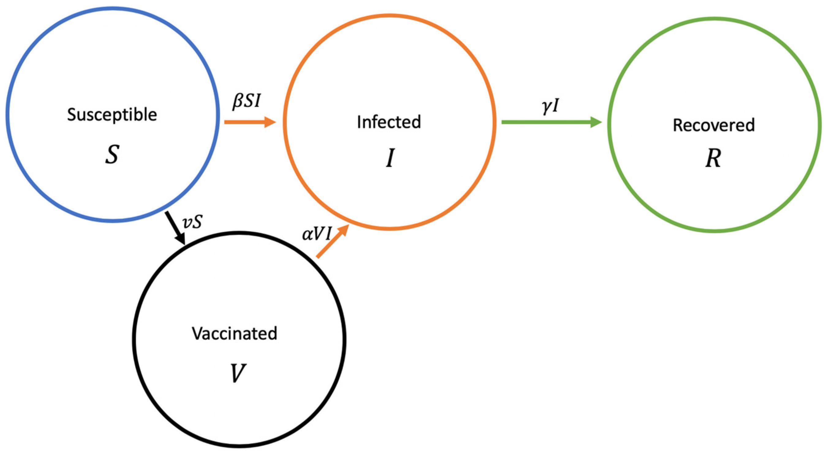
  • We proved the existence and uniqueness of a global solution to a stochastic SIRVI epidemic model incorporating the Ornstein–Uhlenbeck process, and we developed a suitable Lyapunov function to obtain sufficient conditions for persistence in the mean and exponential extinction of infectious disease;
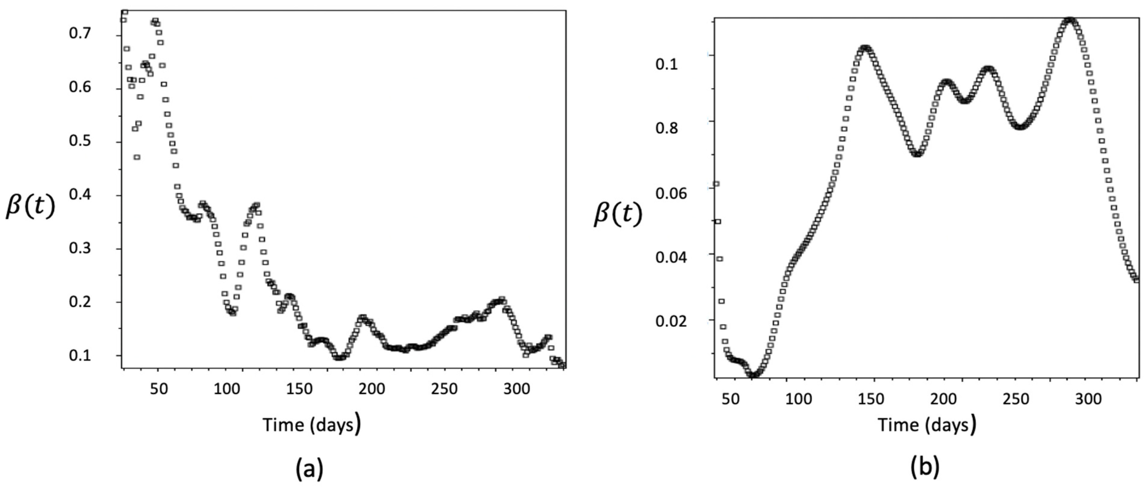
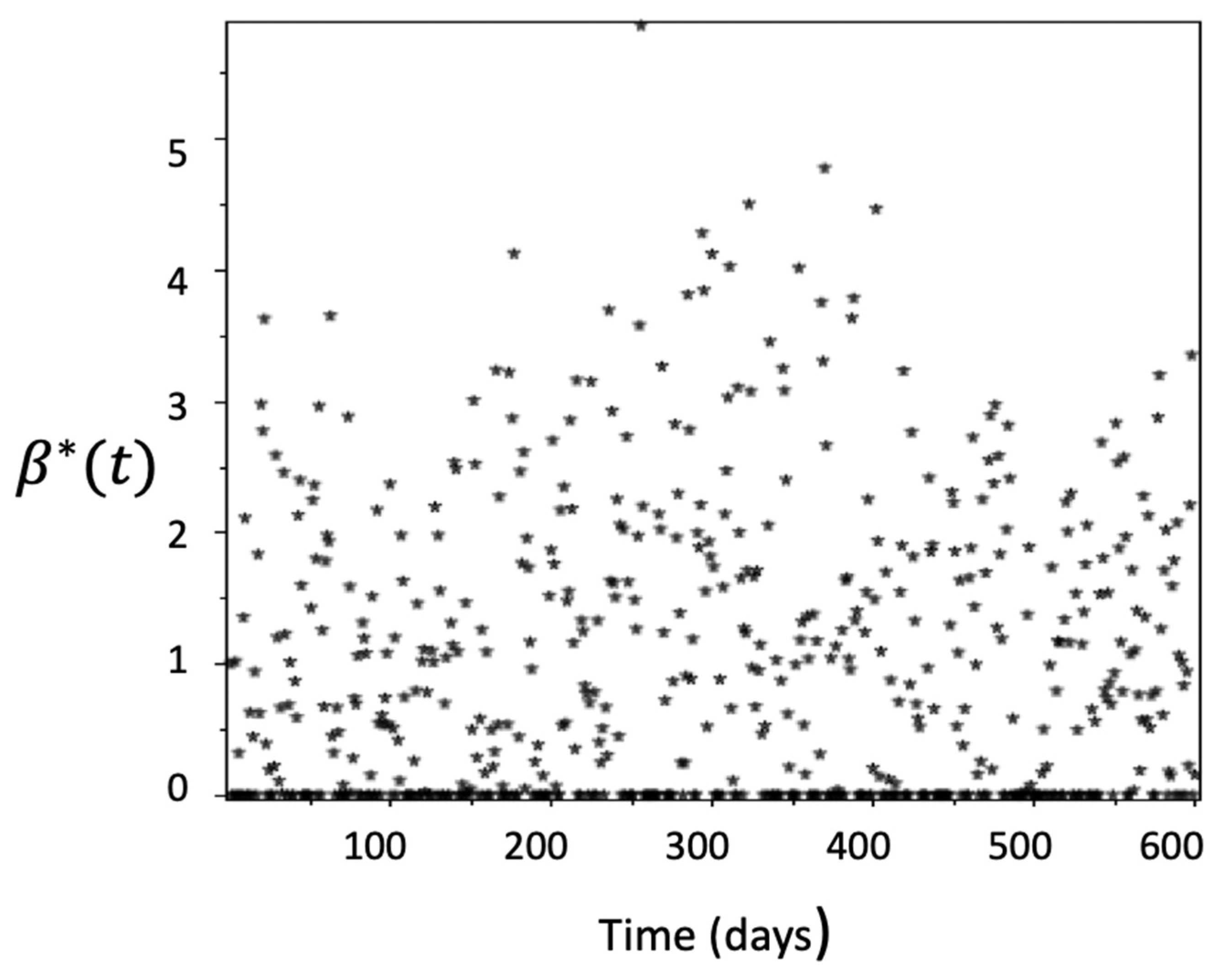
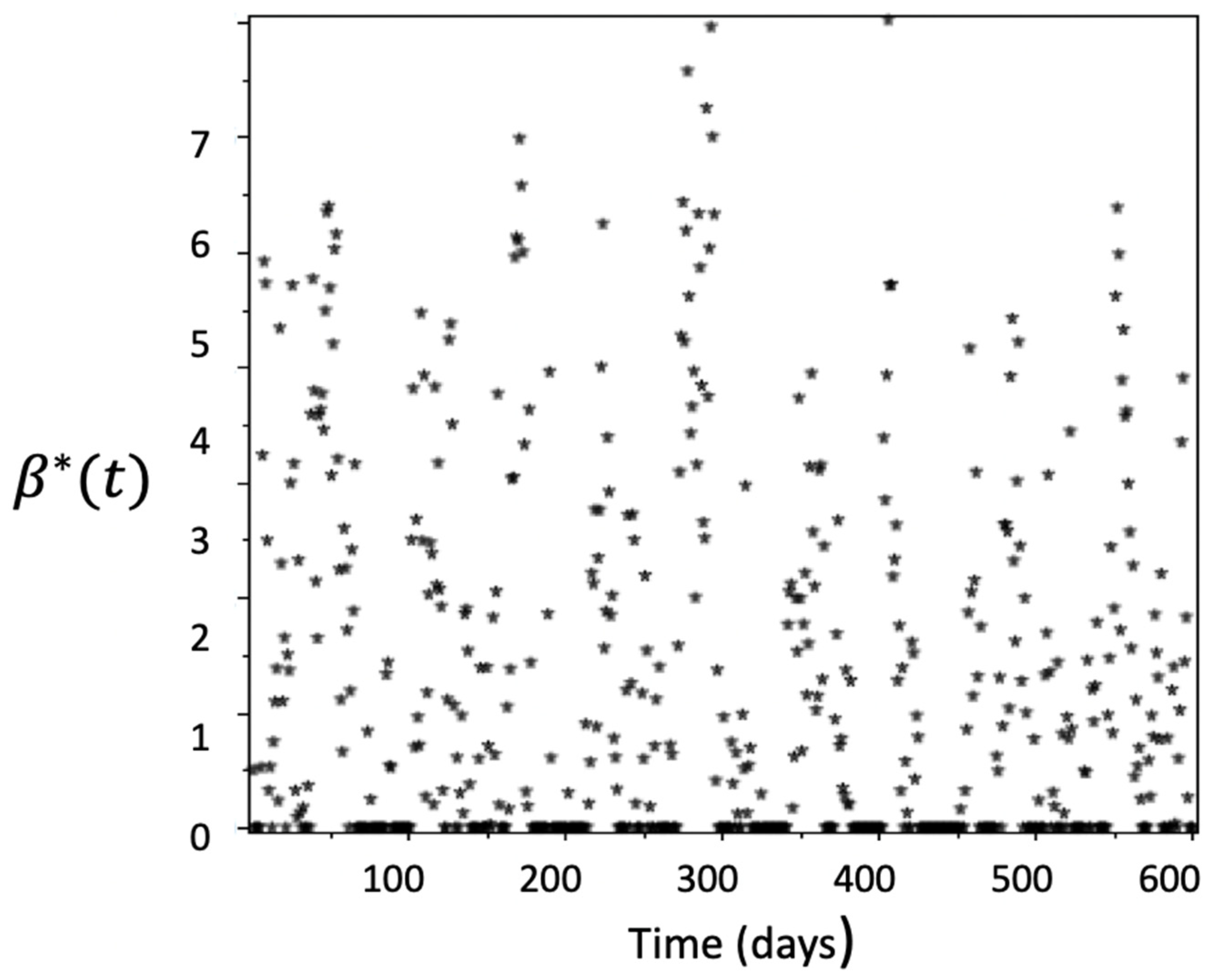
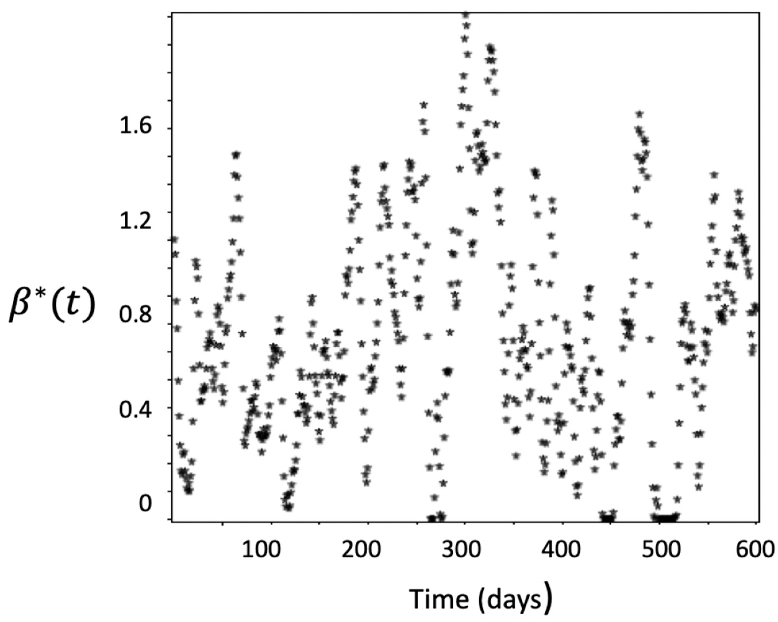
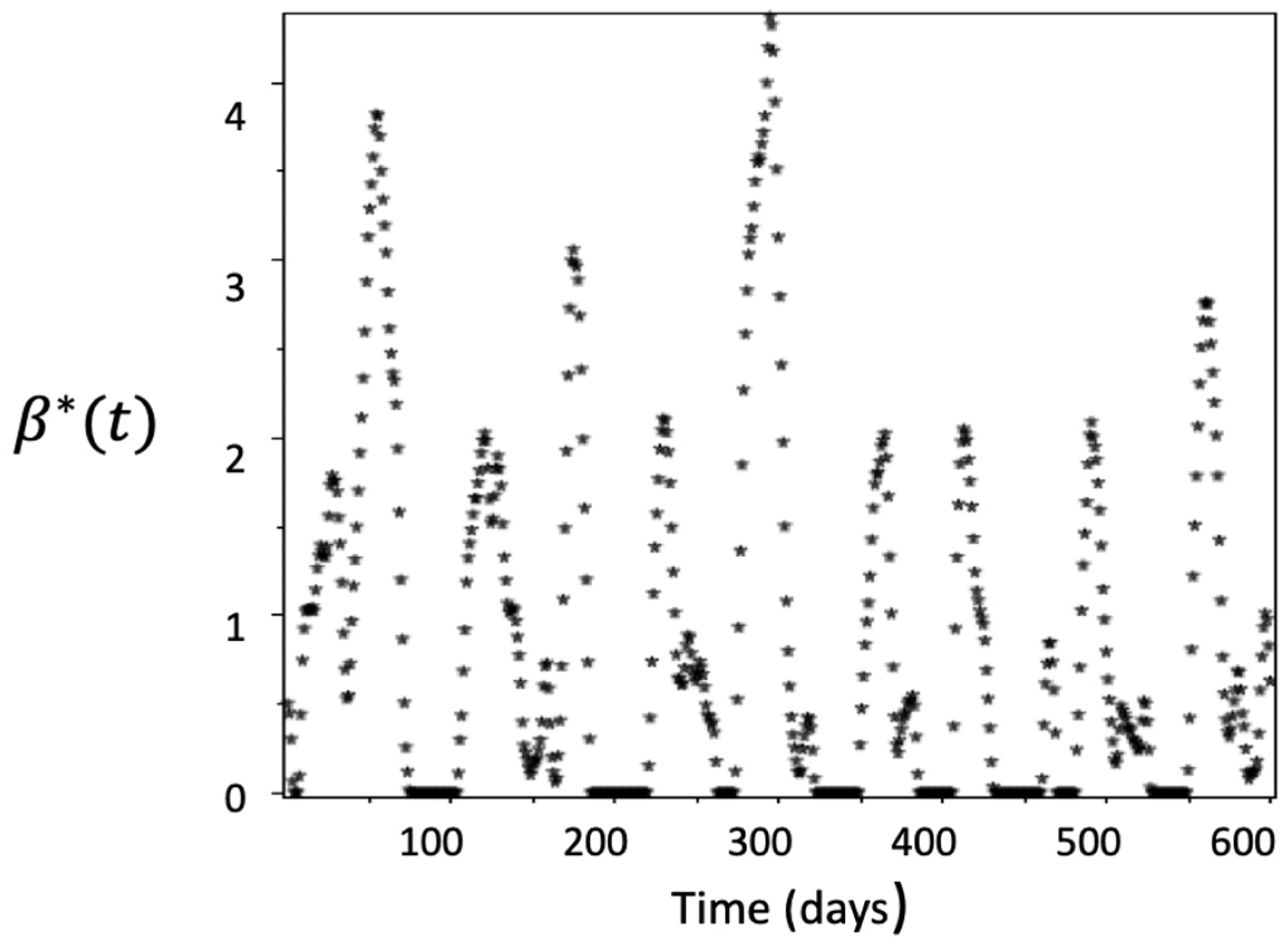
  • The transmission rate is perturbed by the Ornstein–Uhlenbeck process and is numerically solved by using several speed-of-reversion and volatility values. This was compared with the solutions of (23)–(24), and we found that there is no real relationship between the two transmission rates;
  • After using an exponential smoothing technique, we concluded that the transmission rate obtained from the perturbed (from the Ornstein–Uhlenbeck process) system could be represented by a finite linear combination of the Gaussian radial basis function;
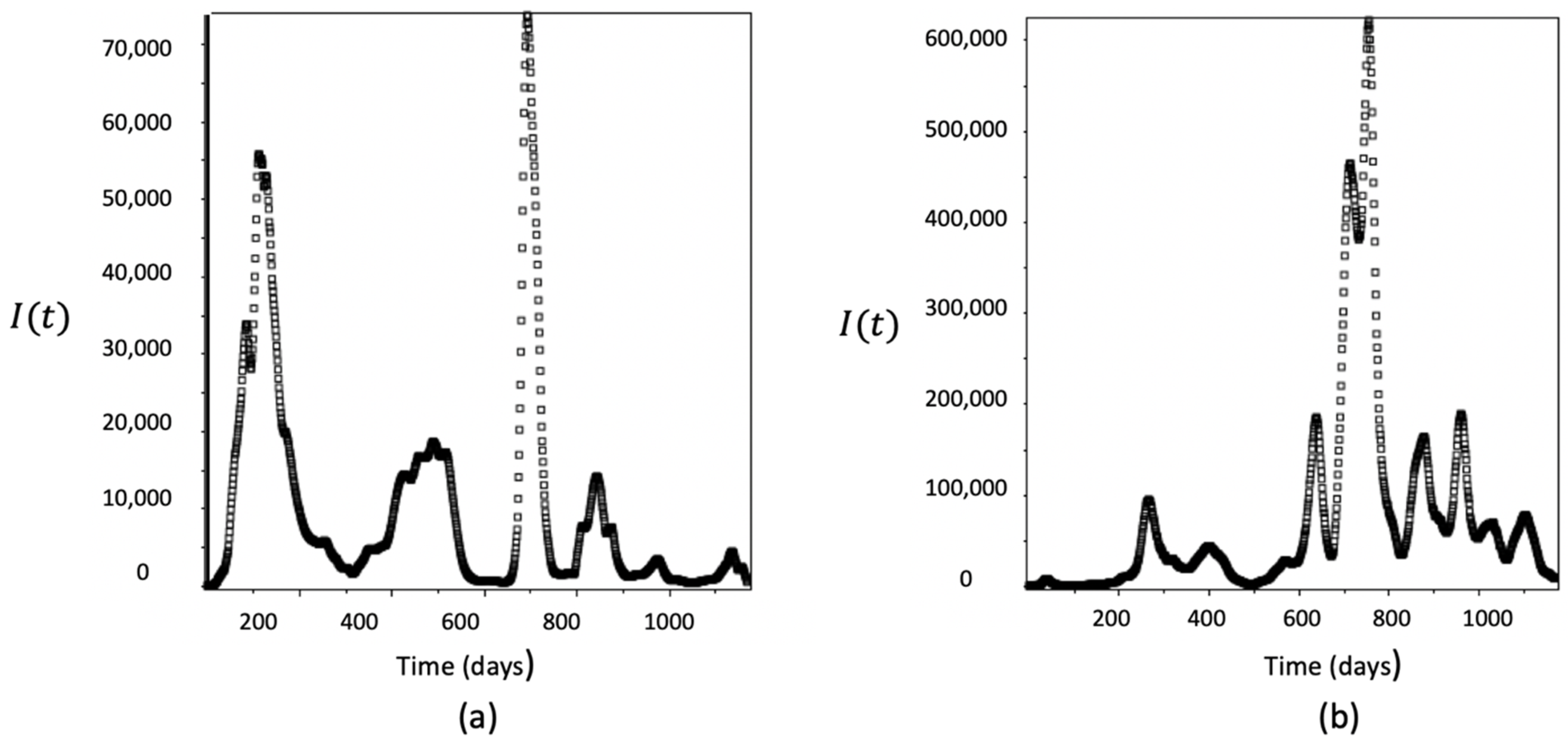
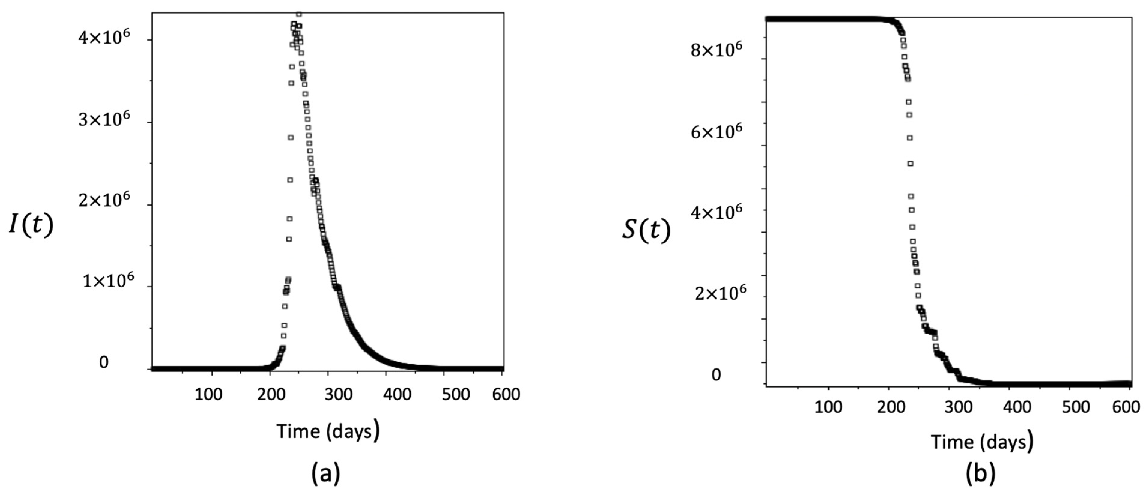
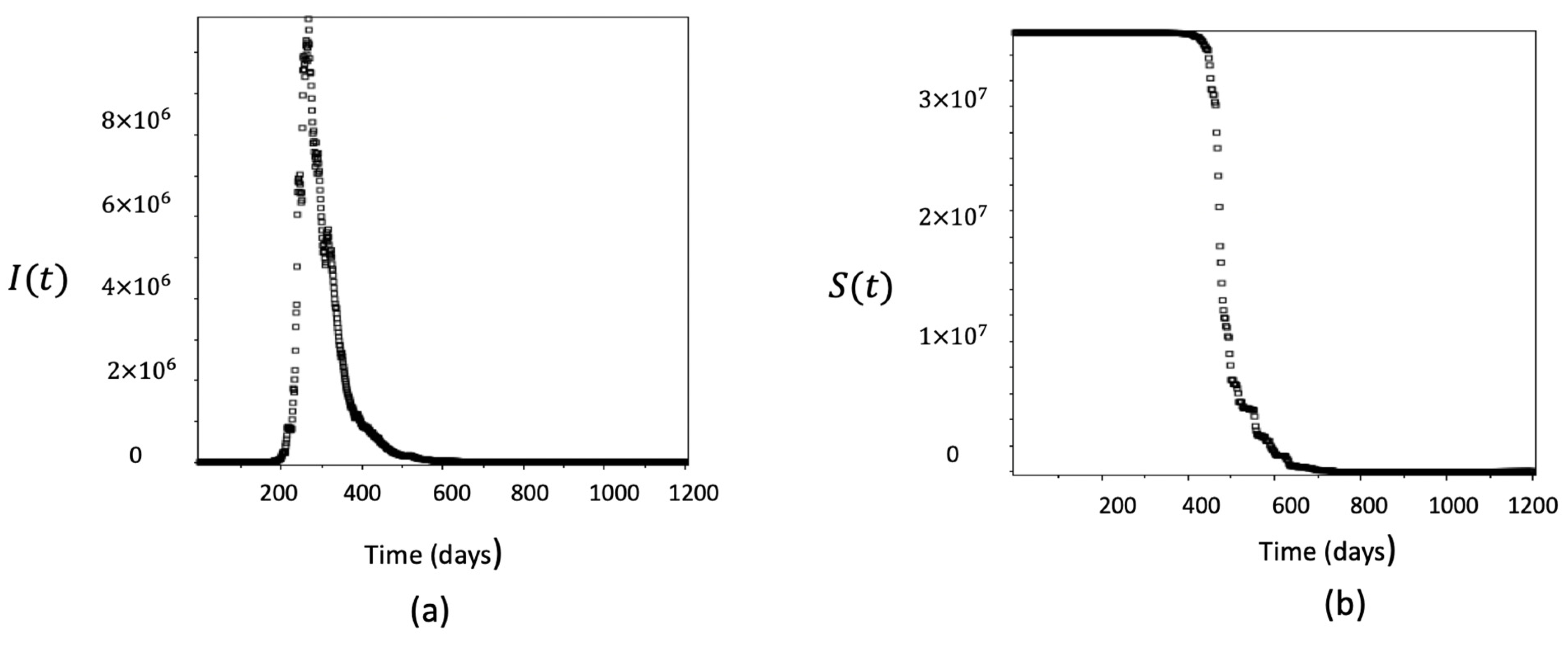
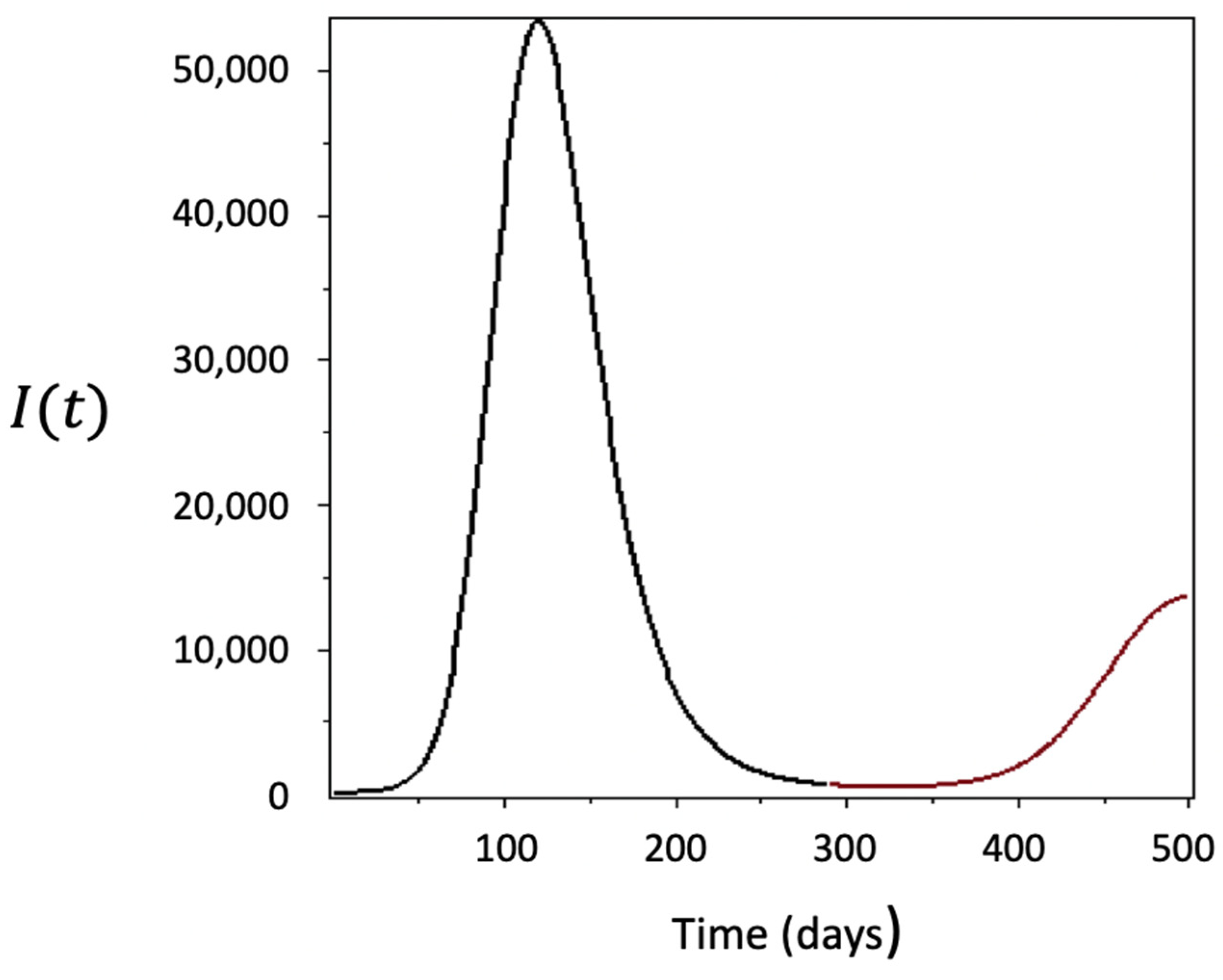
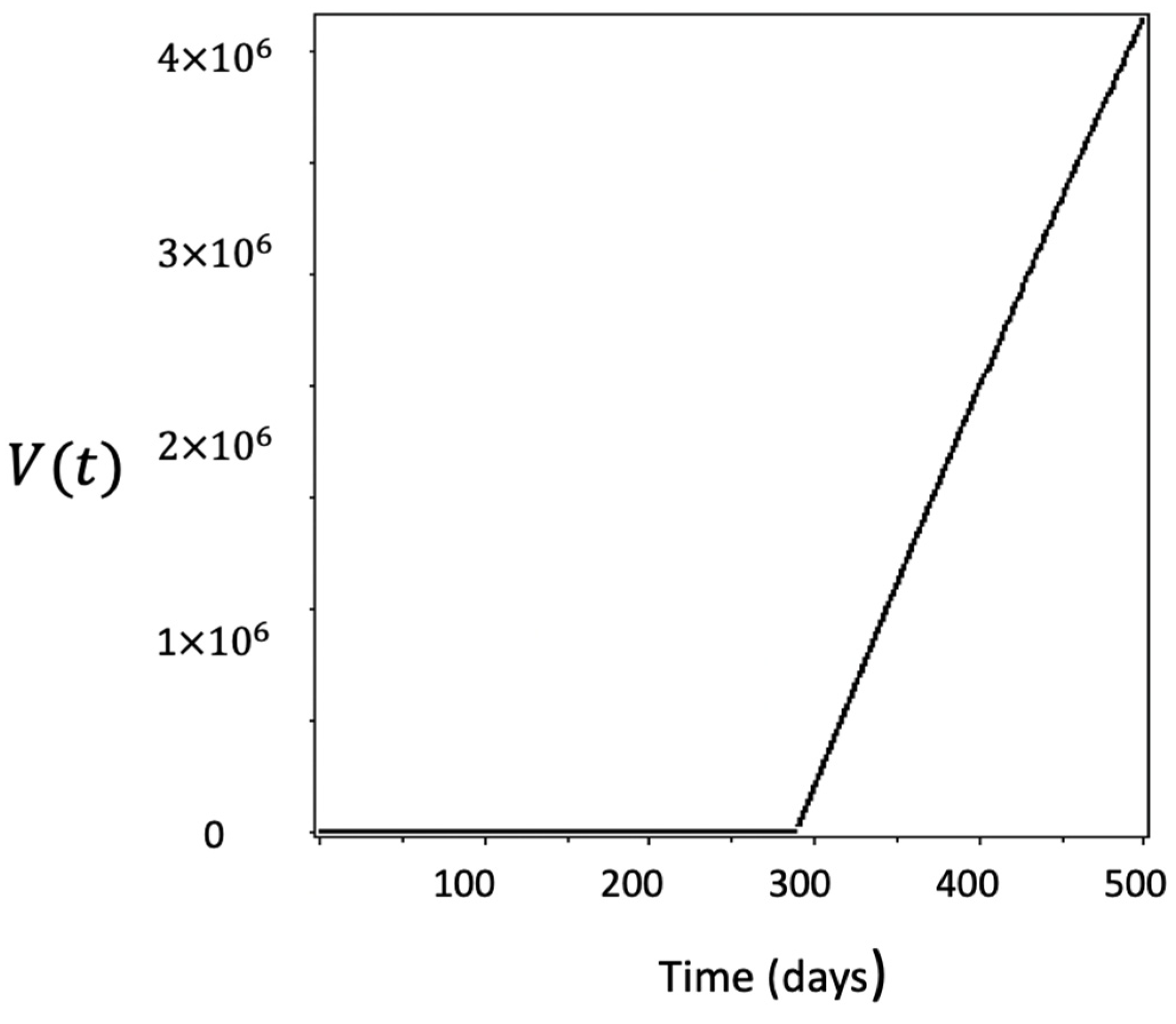
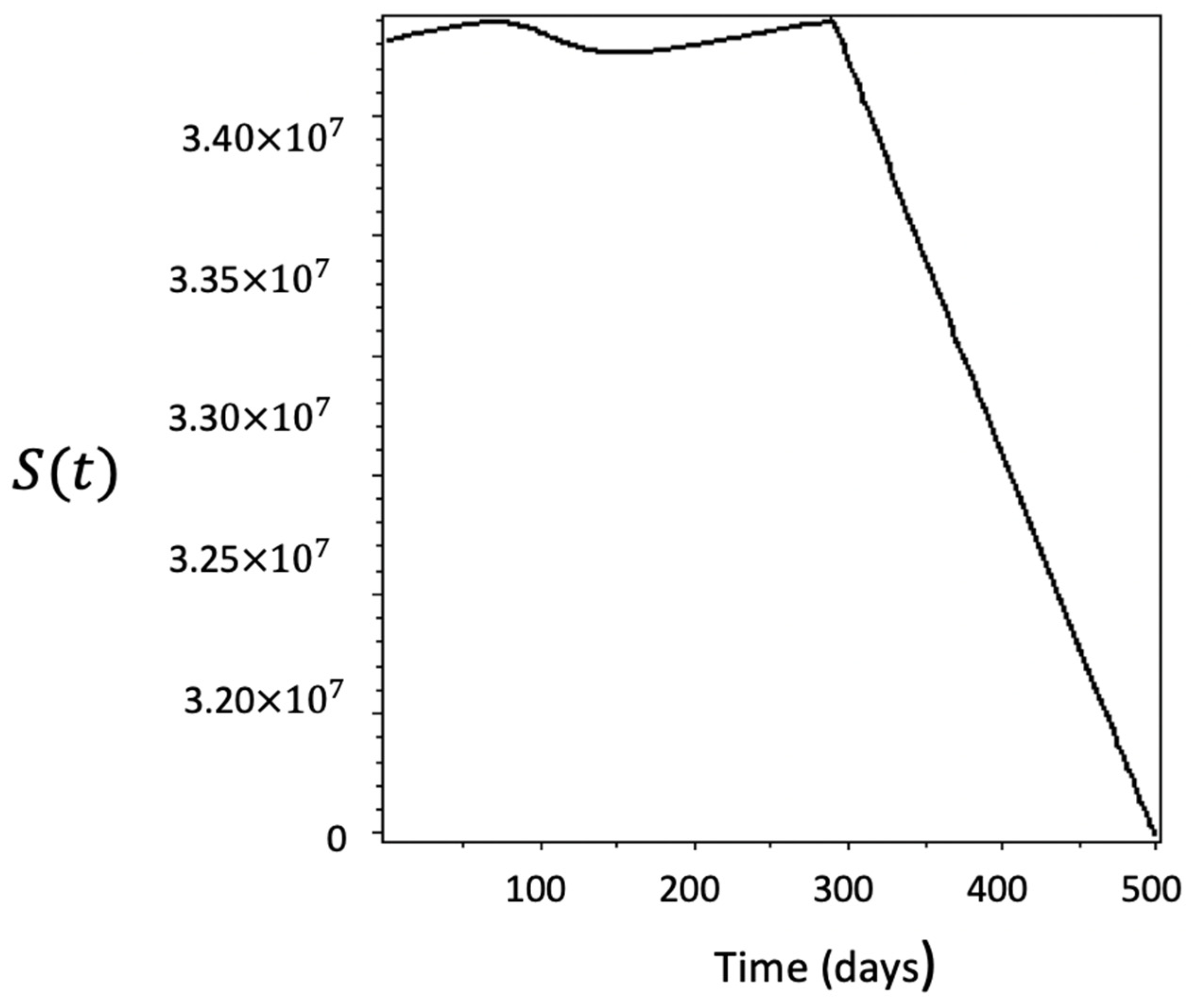
  • The numerical solutions of the stochastic SIRVI epidemic model incorporating the Ornstein–Uhlenbeck process, where the transmission rate is smoothed by using an exponential smoothing technique, predict epidemic waves accurately;
  • The selection of Saudi Arabia and Austria was random, and the method we provided in this paper can be applied to any confirmed daily active cases from any other countries;
  • The theory we developed here can also be used to study any epidemic compartmental models;
  • There are many other parameters involved in epidemic modeling, which are also functions of time. These parameters, such as mortality rate, will be the subject (on the basis of our result) of future research.

Author Contributions

Conceptualization, F.S.A. and F.T.A.; Methodology, F.S.A. and F.T.A.; Software, F.S.A. and F.T.A.; Validation, F.T.A.; Formal analysis, F.T.A.; Writing—original draft, F.S.A. and F.T.A. All authors have read and agreed to the published version of the manuscript.

Funding

This research was funded by the Deputyship for Research & Innovation and the Ministry of Education, Saudi Arabia, through project number IFP-IMSIU202208.

Data Availability Statement

The authors confirm that the data supporting the findings of this study are available within the article.

Acknowledgments

The authors extend their appreciation to the Deputyship for Research & Innovation, Ministry of Education in Saudi Arabia for funding this research work through project number IFP-IMSIU202208.

Conflicts of Interest

The authors declare no conflict of interest.

References

  1. Roberts, M.G.; Heesterbeek, J.A.P. Mathematical models in epidemiology. Math. Model. 2003, 49, 6221. [Google Scholar]
  2. Siettos, C.I.; Russo, L. Mathematical modeling of infectious disease dynamics. Virulence 2013, 4, 295–306. [Google Scholar] [CrossRef] [PubMed]
  3. Krämer, A.; Kretzschmar, M.; Krickeberg, K. (Eds.) Modern Infectious Disease Epidemiology: Concepts, Methods, Mathematical Models, and Public Health; Springer: Berlin/Heidelberg, Germany, 2009; pp. 209–221. [Google Scholar]
  4. Brauer, F. Mathematical epidemiology: Past, present, and future. Infect. Dis. Model. 2017, 2, 113–127. [Google Scholar] [CrossRef] [PubMed]
  5. Kermack, W.O.; McKendrick, A.G. Contributions to the mathematical theory of epidemics I. Bull. Math. Biol. 1991, 53, 33–55. [Google Scholar] [PubMed]
  6. Kermack, W.O.; McKendrick, A.G. Contributions to the mathematical theory of epidemics II. The problem of endemicity. Bull. Math. Biol. 1991, 53, 57–87. [Google Scholar] [PubMed]
  7. Kermack, W.O.; McKendrick, A.G. Contributions to the mathematical theory of epidemics III. Further studies of the problem of endemicity. Bull. Math. Biol. 1991, 53, 89–118. [Google Scholar]
  8. Hethcote, H.W. The Mathematics of Infectious Diseases. SIAM Rev. 2000, 42, 599–653. [Google Scholar] [CrossRef]
  9. Pollard, A.J.; Bijker, E.M. A guide to vaccinology: From basic principles to new developments. Nat. Rev. Immunol. 2020, 21, 83–100. [Google Scholar] [CrossRef]
  10. Rifhat, R.; Teng, Z.; Wang, C. Extinction and persistence of a stochastic SIRV epidemic model with nonlinear incidence rate. Adv. Differ. Equ. 2021, 2021, 200. [Google Scholar] [CrossRef]
  11. Oke, M.O.; Ogunmiloro, O.M.; Akinwumi, C.T.; Raji, R.A. Mathematical Modeling and Stability Analysis of a SIRV Epidemic Model with Non-linear Force of Infection and Treatment. Commun. Math. Appl. 2019, 10, 717–731. [Google Scholar] [CrossRef]
  12. Ishikawa, M. Optimal strategies for vaccination using the stochastic SIRV model. Trans. Inst. Syst. Control Inf. Eng. 2012, 25, 343–348. [Google Scholar] [CrossRef]
  13. Meng, X.; Cai, Z.; Dui, H.; Cao, H. Vaccination strategy analysis with SIRV epidemic model based on scale-free Networks with tunable clustering. IOP Conf. Ser. Mater. Sci. Eng. 2021, 1043, 032012. [Google Scholar] [CrossRef]
  14. Farooq, J.; Bazaz, M.A. A novel adaptive deep learning model of COVİD-19 with focus on mortality reduction strategies. Chaos Solitons Fractals 2020, 138, 110148. [Google Scholar] [CrossRef]
  15. Omae, Y.; Kakimoto, Y.; Sasaki, M.; Toyotani, J.; Hara, K.; Gon, Y.; Takahashi, H. SIRVVD model-based verification of the effect of first and second doses of COVID-19/SARS-CoV-2 vaccination in Japan. Math. Biosci. Eng. 2021, 19, 1026–1040. [Google Scholar] [CrossRef] [PubMed]
  16. Lu, R.; Wei, F. Persistence and extinction for an age-structured stochastic SVIR epidemic model with generalized nonlinear incidence rate. Phys. A Stat. Mech. Its Appl. 2018, 513, 572–587. [Google Scholar] [CrossRef]
  17. Yang, J.; Martcheva, M.; Wang, L. Global threshold dynamics of an SIVS model with waning vaccine-induced immunity and nonlinear incidence. Math. Biosci. 2015, 268, 1–8. [Google Scholar] [CrossRef]
  18. Wen, B.; Teng, Z.; Li, Z. The threshold of a periodic stochastic SIVS epidemic model with nonlinear incidence. Phys. A Stat. Mech. Its Appl. 2018, 508, 532–549. [Google Scholar] [CrossRef]
  19. Turkyilmazoglu, M. An extended epidemic model with vaccination: Weak-immune SIRVI. Phys. A Stat. Mech. Its Appl. 2022, 598, 127429. [Google Scholar] [CrossRef]
  20. Shi, Z.; Zhang, X.; Jiang, D. Dynamics of an avian influenza model with half-saturated incidence. Appl. Math. Comput. 2019, 355, 399–416. [Google Scholar] [CrossRef]
  21. Dai, Y.; Zhou, B.; Jiang, D.; Hayat, T. Stationary distribution and density function analysis of stochastic susceptible-vaccinated-infected-recovered (SVIR) epidemic model with vaccination of newborns. Math. Methods Appl. Sci. 2022, 45, 10991476. [Google Scholar] [CrossRef]
  22. Chang, Z.; Meng, X.; Hayat, T.; Hobiny, A. Modeling and analysis of SIR epidemic dynamics in immunization and cross-infection environments: Insights from a stochastic model. Nonlinear Anal. Model. Control 2022, 27, 740–765. [Google Scholar] [CrossRef]
  23. Lan, G.; Yuan, S.; Song, B. The impact of hospital resources and environmental perturbations to the dynamics of SIRS model. J. Frankl. Inst. 2021, 358, 2405–2433. [Google Scholar] [CrossRef]
  24. Qi, H.; Meng, X. Mathematical modeling, analysis and numerical simulation of HIV: The influence of stochastic environmental fluctuations on dynamics. Math. Comput. Simul. 2021, 187, 700–719. [Google Scholar] [CrossRef]
  25. Allen, E. Environmental variability and mean-reverting processes. Discret. Contin. Dyn. Syst. Ser. B 2016, 21, 2073–2089. [Google Scholar] [CrossRef]
  26. Song, Y.; Zhang, X. Stationary distribution and extinction of a stochastic SVEIS epidemic model incorporating Ornstein–Uhlenbeck process. Appl. Math. Lett. 2022, 133, 108284. [Google Scholar] [CrossRef]
  27. Shi, Z.; Jiang, D. Dynamics and density function of a stochastic differential infectivity epidemic model with Ornstein–Uhlenbeck process. Math. Methods Appl. Sci. 2022, 46, 6245–6261. [Google Scholar] [CrossRef]
  28. Khasminskii, R. Stochastic Stability of Differential Equations; Springer: Berlin, Germany, 2012. [Google Scholar] [CrossRef]
  29. Alshammari, F.S.; Tezcan, E.A. Exploring radial kernel on the novel forced SEYNHRV-S model to capture the second wave of COVID-19 spread and the variable transmission rate. Mathematics 2022, 10, 1501. [Google Scholar] [CrossRef]
  30. Chen, Y.-C.; Lu, P.-E.; Chang, C.-S.; Liu, T.-H. A time-dependent sır model for COVID-19 with undetectable ınfected persons. IEEE Trans. Netw. Sci. Eng. 2020, 7, 3279–3294. [Google Scholar] [CrossRef]
  31. Milstein, G.N. Numerical İntegration of Stochastic Differential Equations, Volume 313 of Mathematics and İts Applications; Translated and Revised from the 1988 Russian Original; Kluwer Academic Publishers Group: Dordrecht, The Netherlands, 1995. [Google Scholar]
Figure 1. The SIRVI epidemic model with main parameters.
Mathematics 11 03876 g001
Figure 2. Active infected individuals (a) Saudi Arabia (b) Austria.
Mathematics 11 03876 g002
Figure 3. Time-dependent transmission rate for (a) Saudi Arabia and (b) Austria.
Mathematics 11 03876 g003
Figure 4. Time-dependent transmission rate perturbed by the Ornstein–Uhlenbeck process, where β * ( t ) = M a x { β ( t ) , 0 } .
Mathematics 11 03876 g004
Figure 5. Time-dependent transmission rate perturbed by the Ornstein–Uhlenbeck process, where β * ( t ) = M a x { β ( t ) , 0 } .
Mathematics 11 03876 g005
Figure 6. Obtained from Figure 3 by using exponential smoothing.
Mathematics 11 03876 g006
Figure 7. Obtained from Figure 3 by using exponential smoothing.
Mathematics 11 03876 g007
Figure 8. Numerical solution of Equation (26) for Austria: (a) infected individual I(t); (b) suspectable population.
Mathematics 11 03876 g008
Figure 9. Numerical solution of Equation (26) for Saudi Arabia: (a) infected individual I(t); (b) susceptible population.
Mathematics 11 03876 g009
Figure 10. Active infected population (numerical solution to (26) with (27)).
Mathematics 11 03876 g010
Figure 11. Plot of vaccinated population.
Mathematics 11 03876 g011
Figure 12. Plot of suspectable population.
Mathematics 11 03876 g012
Disclaimer/Publisher’s Note: The statements, opinions and data contained in all publications are solely those of the individual author(s) and contributor(s) and not of MDPI and/or the editor(s). MDPI and/or the editor(s) disclaim responsibility for any injury to people or property resulting from any ideas, methods, instructions or products referred to in the content.

