Fixed/Preassigned-Time Stochastic Synchronization of Complex-Valued Fuzzy Neural Networks with Time Delay

Abstract

Instead of the separation approach, this paper mainly centers on studying the fixed/preassigned-time (FXT/PAT) synchronization of a type of complex-valued stochastic fuzzy cellular neural networks (CVSFCNNs) with time delay based on the direct method. Firstly, some basic properties of the sign function in complex fields and some generalized FXT/PAT stability lemmas for nonlinear stochastic differential equations are introduced. Secondly, by designing two delay-dependent complex-valued controllers with/without a sign function, sufficient conditions for CVSFCNNs to achieve FXT/PAT synchronization are obtained. Finally, the feasibility of the theoretical results is verified through a numerical example.

1. Introduction

It is well known that Chua and Yang first introduced a fuzzy neural network in 1988 [1,2]. Since then, fuzzy neural networks (FNNs) have aroused high interest among researchers due to their widespread applications in many areas, such as visual microprocessors, image processing, and other fields [3,4]. In practice, the indeterminacy or ambiguity of non-linear dynamic systems is unavoidable. To account for ambiguity, Yang et al. further introduced the so-called fuzzy cellular neural networks (FCNNs) in 1996 [5]. Numerous experiments have shown that FCNNs are an excellent example of processing and pattern recognition. Therefore, studying the dynamic behavior of FCNNs is an interesting and vital research topic in theory and in application. Moreover, researchers have extensively considered the stability and synchronization of various types of FCNNs and have published many excellent papers [6,7,8,9].

As an extension of real-valued neural networks (RVNNs), complex-valued neural networks (CVNNs) were developed by substituting real-valued parameters with complex-valued parameters and, in recent years, have aroused great enthusiasm among scholars. Facts have proven that they can handle many problems, such as symmetry detection and electromagnetic wave imaging [10,11], which cannot be solved in RVNNs. As a result, many scholars have studied the dynamic behavior of CVNNs due to their applications in fields such as secure communication, signal processing, and control systems [12,13,14]. For example, in [14], the FXT synchronization of complex-valued memristive bidirectional associative memory neural networks (BAMNNs) and applications in image encryption and decryption was studied. In [15], the authors mainly studied the FXT synchronization for complex-valued BAMNNs with time delays. Additionally, in [16,17], the finite-time (FNT) and FXT synchronization of CVNNs was studied by the non-separation method. The papers [18,19] discuss the performance of a deep belief network and a multilayer long short-term memory (LSTM)network. However, the networks discussed in these articles are a type of specific neural network structure, which is used for unsupervised learning, feature extraction, and processing sequence data, such as time series or continuous action sequences. In practical applications, CVNNs can also be considered and studied for similar problems. Such research can further explore how to use CVNNs to improve the performance of long-distance iris recognition tasks. Unfortunately, random interference has not been considered in these works. The availability of many natural renewable resources, such as wind and sunlight, will be disrupted to an extent by random disturbances [20]. Therefore, the study of CVNNs with random perturbation has important practical significance.

Additionally, the study of synchronization of nonlinear systems has been highly regarded and extensively studied in the last three decades [21,22,23,24,25,26]. However, in practical applications, the synchronization of complex-valued fuzzy cellular neural networks (CVFCNNs) has broader application prospects than general neural networks (NNs). For example, in communication systems, solving synchronization problems can effectively improve the accuracy and stability of data transmission, thereby improving the performance of communication systems. Secondly, the synchronization ability of CVFCNNs can be used to achieve collaborative operations between multiple control systems, improving the accuracy and robustness of control systems. Therefore, in the context of existing literature and practical applications, studying the synchronization problem of CVFCNNs is a significant related research direction. The settling time (ST) in FNT synchronization depends largely on the initial state; however, in practical applications, we cannot obtain the initial condition in advance. Therefore, to make up for this deficiency, Polyakov proposed the concept of FXT stability in 2012 [27], and the FXT synchronization of NNs in the complex field has been extensively studied [14,15,28,29]. In 2021, Hu et al. introduced an improved FXT stability method [30]. This method shows that the ST of PAT synchronization is not dependent on the initial state of the discussed system or on the values of the controller parameters in question. Nevertheless, up to now, research on the PAT synchronization of CVSFCNNs has not been reported. This has inspired us to undertake relevant research.

Time delay is an automatic characteristic of many dynamic models. It has been recognized that time delays often occur in signal transmission between different neurons. In [15,16,17,31], the FXT synchronization of CVNNs is studied with or without stochastic effects. The article [16], involving discontinuous activation and time-varying delays, mainly studied the problem of synchronization in FNT/FXT for fully complex-variable delayed NNs. The paper [17] developed a non-separation approach and explored the problem of FNT/FXT synchronization for fully complex-valued dynamical networks. In [31], the author mainly studied the FXT/PAT synchronization problem of CVBAM NNs with random disturbances and impulsive effects. Nevertheless, the controllers designed in these articles all contain sign functions. As far as we know, the chattering effect will occur in the system due to the discontinuity of the sign function when synchronization is implemented. Therefore, this encourages us to design a controller that does not contain a sign function, which is also a highlight of this paper.

Considering the above discussions, for CVSFCNNs with time delay, FXT/PAT synchronization has not been fully resolved. Therefore, this paper will deeply explore the FXT/PAT synchronization of CVSFCNNs. The innovations of this paper can be summarized as: (i) Considering the universality of stochastic and time-delay effects in real life, this paper first investigates the stochastic synchronization problem of CVNNs with time delay; (ii) unlike previous works [14,15,32], this paper studies the synchronization of the SFCNNs by using the direct method instead of the separation method. Moreover, the controllers constructed in this article do not contain the sign function, thus effectively avoiding the vibrations caused by the sign function.

The remaining parts of this article are structured as follows. The relevant definitions, assumptions, and essential lemmas are given in Section 2. The primary research process and results of this paper are shown in Section 3. In Section 4, a numerical example is used to prove the correctness of the theoretical results. Finally, Section 5 summarizes this paper and provides the future research directions.

Notations. The symbols $\mathcal{R}$, $\mathcal{C}$, ${\mathcal{R}}^{\mathrm{n}}$, and ${\mathcal{C}}^{\mathrm{n}}$ denote all real numbers, complex numbers, all n-dimensional real vectors, and all n-dimensional complex vectors. For any $s\in \mathcal{C},\overline{s}$ denotes the conjugate of s, and $Re\left(s\right)$ and $Im\left(s\right)$ denote the real and imaginary parts of s, respectively. ${|s|}_2=\sqrt{s\overline{s}}$, while i denotes the imaginary unit with $i^2=-1$.

2. Problem Formulation and Preliminary Description

In the following, we study the case of $\mathrm{m}$-dimensions of CVSFCNNs:

$$\left\{\begin{array}{cc}\hfill d{x}_i\left(t\right)=& [-a_i{x}_i\left(t\right)+\sum _{\ell =1}^{\mathrm{m}}{p}_{i\ell }{f}_{\ell }\left(x_{\ell }\left(t\right)\right)+\sum _{\ell =1}^{\mathrm{m}}{b}_{i\ell }{f}_{\ell }\left(x_{\ell }(t-{\tau }_{\ell }\left(t\right))\right)\hfill \\ & +\sum _{\ell =1}^{\mathrm{m}}{r}_{i\ell }{v}_{\ell }+\underset{\ell =1}{\overset{\mathrm{m}}{\bigwedge }}{\alpha }_{i\ell }{f}_{\ell }\left(x_{\ell }(t-{\tau }_{\ell }\left(t\right))\right)+\underset{\ell =1}{\overset{\mathrm{m}}{\bigwedge }}{T}_{i\ell }{v}_{\ell }\hfill \\ \hfill & +\underset{\ell =1}{\overset{\mathrm{m}}{\bigvee }}{\beta }_{i\ell }{f}_{\ell }\left(x_{\ell }(t-{\tau }_{\ell }\left(t\right))\right))+\underset{\ell =1}{\overset{\mathrm{m}}{\bigvee }}{S}_{i\ell }{v}_{\ell }+I_i]dt\hfill \\ \hfill & +{\sigma }_i\left(x_i\left(t\right),t\right)d\omega \left(t\right),\hfill \\ \hfill x_i\left(t\right)=& x_i^0\in \mathcal{C},i=1,2,\dots ,\mathrm{m},\hfill \end{array}\right.$$

(1)

wherein $x_i\left(t\right)\in \mathcal{C}$ represents the state variables of the ith neuron; $a_i\in \mathcal{C}$ is the self-inhibition of the ith neuron; $f_{\ell }(·)\in \mathcal{C}$ represents the activation functions; ${\tau }_{\ell }\left(t\right)$ is the time-varying delay, which satisfies ${\acute{\tau }}_{\ell }\left(t\right)<{\tau }_1<1$; $p_{i\ell }\in \mathcal{C},b_{i\ell }\in \mathcal{C}$ represent the connection weights; and $r_{i\ell },T_{i\ell },S_{i\ell },{\alpha }_{i\ell }$, and ${\beta }_{i\ell }$ are the elements of the feed-forward template, fuzzy feed-forward minimum template, fuzzy feed-forward maximum template, fuzzy feedback minimum template, and fuzzy feedback maximum template, respectively. ⋀ and ⋁ correspond to the fuzzy AND and OR operations; $I_i\in \mathcal{C}$ and $v_{\ell }\in \mathcal{C}$ are the inputs and bias of the ith neuron; ${\sigma }_i(·,t):\mathcal{C}\times R^{+}\to \mathcal{C}$ denotes the noise intensity functions; and $\omega \left(t\right)\in \mathcal{C}$ represents the one-dimensional Brownian motion defined on a complete probability space $(\mathrm{\Omega },F,P)$ with a natural filtration ${\left\{F_t\right\}}_t\ge 0$ generated by $\omega \left(e\right):0\le e\le t$.

Remark 1.

In CVSFCNNs (1), fuzzy AND and fuzzy OR operations are defined as follows:

$$\begin{array}{cc}\hfill \underset{\ell =1}{\overset{\mathrm{m}}{\bigwedge }}{\alpha }_{i\ell }{f}_{\ell }\left(x_{\ell }\left(t\right)\right)& \le \underset{1\le \ell \le \mathrm{m}}{min}\left\{{\alpha }_{i\ell }{f}_{\ell }\left(x_{\ell }\left(t\right)\right)\right\},\hfill \\ \hfill \underset{\ell =1}{\overset{\mathrm{m}}{\bigvee }}{\beta }_{i\ell }{f}_{\ell }\left(x_{\ell }\left(t\right)\right)& \le \underset{1\le \ell \le \mathrm{m}}{max}\left\{{\beta }_{i\ell }{f}_{\ell }\left(x_{\ell }\left(t\right)\right)\right\},\hfill \end{array}$$

and for fuzzy AND and OR operations, the upper and lower limits are defined as follows [33]:

$$\begin{array}{cc}\hfill sup(A\bigwedge B)& =min(A,B),\hfill \\ \hfill inf(A\bigwedge B)& =A\ast B,\hfill \\ \hfill sup(A\bigvee B)& =max(A,B),\hfill \\ \hfill inf(A\bigvee B)& =A+B-A\ast B.\hfill \end{array}$$

In this article, we investigate drive–response synchronization. The response system corresponding to the drive system (1) is:

$$\left\{\begin{array}{cc}\hfill d{y}_i\left(t\right)=& [-a_i{y}_i\left(t\right)+\sum _{\ell =1}^{\mathrm{m}}{p}_{i\ell }{f}_{\ell }\left(y_{\ell }\left(t\right)\right)+\sum _{\ell =1}^{\mathrm{m}}{b}_{i\ell }{f}_{\ell }\left(y_{\ell }(t-{\tau }_{\ell }\left(t\right))\right)\hfill \\ & +\sum _{\ell =1}^{\mathrm{m}}{r}_{i\ell }{v}_{\ell }+\underset{\ell =1}{\overset{\mathrm{m}}{\bigwedge }}{\alpha }_{i\ell }{f}_{\ell }\left(y_{\ell }(t-{\tau }_{\ell }\left(t\right))\right)+\underset{\ell =1}{\overset{\mathrm{m}}{\bigwedge }}{T}_{i\ell }{v}_{\ell }\hfill \\ \hfill & +\underset{\ell =1}{\overset{\mathrm{m}}{\bigvee }}{\beta }_{i\ell }{f}_{\ell }\left(y_{\ell }(t-{\tau }_{\ell }\left(t\right))\right))+\underset{\ell =1}{\overset{\mathrm{m}}{\bigvee }}{S}_{i\ell }{v}_{\ell }+I_i+u_i\left(t\right)]dt\hfill \\ \hfill & +{\sigma }_i\left(y_i\left(t\right),t\right)d\omega \left(t\right),\hfill \\ \hfill y_i\left(t\right)=& y_i^0\in \mathcal{C},i=1,2,\dots ,\mathrm{m},\hfill \end{array}\right.$$

(2)

wherein $y_i\left(t\right)$ represents the state variable of the response system (2), $u_i\left(t\right)$ represents the control scheme, and $y_i^0\in \mathcal{C}$ represents the initial state of system (2).

If we set $e_i\left(t\right)=y_i\left(t\right)-x_i\left(t\right)$, then we can obtain the following error system:

$$\left\{\begin{array}{cc}\hfill d{e}_i\left(t\right)=& [-a_i{e}_i\left(t\right)+\sum _{\ell =1}^{\mathrm{m}}{p}_{i\ell }{f}_{\ell }\left(e_{\ell }\left(t\right)\right)+\sum _{\ell =1}^{\mathrm{m}}{b}_{i\ell }{f}_{\ell }\left(e_{\ell }(t-{\tau }_{\ell }\left(t\right))\right)\hfill \\ & +\underset{\ell =1}{\overset{\mathrm{m}}{\bigwedge }}{\alpha }_{i\ell }{f}_{\ell }\left(e_{\ell }(t-{\tau }_{\ell }\left(t\right))\right)+\underset{\ell =1}{\overset{\mathrm{m}}{\bigvee }}{\beta }_{i\ell }{f}_{\ell }\left(e_{\ell }(t-{\tau }_{\ell }\left(t\right))\right))+u_i]dt\hfill \\ \hfill & +{\sigma }_i\left(e_i\left(t\right),t\right)d\omega \left(t\right),\hfill \\ \hfill e_i\left(t\right)=& e_i^0\in \mathcal{C},i=1,2,\dots ,\mathrm{m},\hfill \end{array}\right.$$

(3)

where $f\left(e_{\ell }\left(t\right)\right)=f_{\ell }\left(y_{\ell }\left(t\right)\right)-f_{\ell }\left(x_{\ell }\left(t\right)\right)$.

Below, we introduce the relevant presuppositions and then use these methods to derive the main results of the system studied in this article.

Assumption 1.

Noise function ${\sigma }_i(t,·)$ has a positive number ${\eta }_i$, making the following inequality hold true:

$$\frac{1}{2}{\sigma }_i(t,f\left(t\right))\overline{{\sigma }_i(t,f\left(t\right))}\le \sum _{i=1}^{\mathrm{m}}{\eta }_i{|f\left(t\right)|}_2^2.$$

Definition 1

([34]). System (1) is said to be synchronized with system (2) in FXT if there exists a fixed settling time $T_0$ that is independent of the initial synchronization error such that ${lim}_{t\to T_0}E\left(e_i\left(t\right)\right)=0$, and $e_i\left(t\right)\equiv 0$ for $t>T_0$, $i=1,2,\dots ,\mathrm{m}$.

Definition 2

([35]). For any $\kappa \in \mathcal{C},\left[\kappa \right]=sign\left(Re\right(\kappa \left)\right)+isign\left(Im\right(\kappa \left)\right)$ is said to be the sign function of κ.

Definition 3

([36]). For any suitable cone $\Xi \in {\mathcal{R}}^{\mathrm{n}}$, the partial ordering relation derived by Ξ in $R^n$ can be defined as follows:

(i) 

$f⪰h\iff f-h\in \Xi$,

(ii) 

$f\succ h\iff f-h\in int\Xi$,

where the interior of Ξ is represented by $int\Xi$.

Remark 2.

The above method can conveniently determine the “size” of any two vectors. Since a complex vector can be regarded as a two-dimensional real vector, Definition 3 can also be used to compare the "size" of complex numbers. For instance, for any two different complex numbers $z_1=a+bi,z_2=c+di$, define the following relationships:

(i) 

If $a>(<)c$ and $b\ne d$, then $z_1\succ (\prec )z_2$,

(ii) 

If $a>(<)c,b=d$, or $a=c,b>(<)d$, then $z_1⪰(⪯)z_2$,

(iii) 

If $a=c$ and $b=d$, then $z_1=z_2$.

Lemma 1

([35]). If there exists a C-regular function $V\left(z\left(t\right)\right):{\mathcal{R}}^{\mathrm{n}}\to \mathcal{R}$, and the inequality

$$\pounds V\left(z\left(t\right)\right)\le kV\left(z\left(t\right)\right)-\chi V^{\varrho }\left(z\left(t\right)\right)-\psi V^{\rho }\left(z\left(t\right)\right),z\left(t\right)\in R^{\mathrm{n}}\backslash \left\{0\right\}$$

holds true, where $\chi >0,\psi >0$, $0\le \rho <1<\varrho$, then the origin of system (3) is FXT stable in probability, and its ST can be reckoned as $E\left[T(e_0,\omega )\right]<T_{max}$, where

$${\displaystyle T_{max}\triangleq \left\{\begin{array}{ccc}{T}_{max}^1=\hfill & {\displaystyle \frac{1}{k\lambda (1-\varrho )}ln\left(1-\frac{k}{\psi }{\left(\frac{\psi }{\chi }\right)}^{\lambda }\right),}\hfill & {\displaystyle k<0,}\hfill \\ T_{max}^2=\hfill & {\displaystyle \frac{\pi }{(\varrho -\rho )\psi }{\left(\frac{\psi }{\chi }\right)}^{\lambda }csc\left(\lambda \pi \right),}\hfill & {\displaystyle k=0,}\hfill \\ T_{max}^3=\hfill & {\displaystyle \frac{\pi csc\left(\lambda \pi \right)}{\chi (\varrho -\rho )}{\left(\frac{\chi }{\psi -k}\right)}^{1-\lambda }I\left(\frac{\chi }{\gamma },\lambda ,1-\lambda \right)}\hfill & \\ \hfill & {\displaystyle +\frac{\pi csc\left(\lambda \pi \right)}{\psi (\varrho -\rho )}{\left(\frac{\psi }{\chi -k}\right)}^{\lambda }I\left(\frac{\psi }{\gamma },1-\lambda ,\lambda \right),}\hfill & {\displaystyle 0<k<min\{\chi ,\psi \},}\hfill \end{array}\right.}$$

and where $\lambda =\frac{(1-\rho )}{(\varrho -\rho )}$, $\gamma =\chi +\psi -k$. In particular, when $\varrho +\rho =2$, ST can be more accurately estimated as $T(z_0,\omega )<{\tilde{T}}_{max}$, where

$${\displaystyle {\tilde{T}}_{max}\triangleq \left\{\begin{array}{ccc}{T}_{max}^4=\hfill & {\displaystyle \frac{1}{\varrho -1}\frac{2}{\sqrt{\vartheta }}\left(\frac{\pi }{2}+arctan\left(\frac{k}{\sqrt{\vartheta }}\right)\right),}\hfill & {\displaystyle -2\sqrt{\chi \psi }<k<2\sqrt{\chi \psi }}\hfill \\ T_{max}^5=\hfill & {\displaystyle \frac{2}{k(\varrho -1)},}\hfill & {\displaystyle k=-2\sqrt{\chi \psi },}\hfill \\ T_{max}^6=\hfill & {\displaystyle \frac{1}{(\varrho -1)\sqrt{-\vartheta }}ln\frac{k+\sqrt{-\vartheta }}{k-\sqrt{-\vartheta }},}\hfill & {\displaystyle k<-2\sqrt{\chi \psi },}\hfill \end{array}\right.}$$

and where $\vartheta =4\chi \psi -k^2$.

Lemma 2

([35]). If there exists a C-regular function $V\left(z\left(t\right)\right):{\mathcal{R}}^{\mathrm{n}}\to \mathcal{R}$ satisfying the inequality

$$\pounds V\left(z\left(t\right)\right)\le \frac{\overline{T}}{T_p}\left(kV\left(z\left(t\right)\right)-\chi V^{\varrho }\left(z\left(t\right)\right)-\psi V^{\rho }\left(z\left(t\right)\right)\right),z\left(t\right)\in R^{\mathrm{n}}\backslash \left\{0\right\},$$

then the error system (3) is PAT stable in probability within a PAT $T_p>0$, where

$${\displaystyle \overline{T}\triangleq \left\{\begin{array}{cc}{\displaystyle T_{max},}\hfill & {\displaystyle if\varrho +\rho \ne 2,}\hfill \\ {\displaystyle {\tilde{T}}_{max},}\hfill & if\varrho +\rho =2.\hfill \end{array}\right.}$$

Lemma 3

([17]). For any $\kappa \in \mathcal{C},h\left(t\right)\in co\left(\right[r\left(t\right)\left]\right)$, the following inequality holds:

(1) 

$\kappa +\overline{\kappa }=2Re\left(\kappa \right)\le 2{|\kappa |}_2$,

(2) 

$\overline{\left[r\right(t\left)\right]}r\left(t\right)+\left[r\left(t\right)\right]\overline{r\left(t\right)}\ge 2{|r\left(t\right)|}_2$,

(3) 

$\overline{r\left(t\right)}h\left(t\right)+r\left(t\right)\overline{h\left(t\right)}\ge 2{|r\left(t\right)|}_2$.

Lemma 4

([37]). If $e_1,e_2,\cdots ,e_{\mathrm{m}}\ge 0,0<\epsilon \le 1,ϵ>1$, then

$$\sum _{s=1}^{\mathrm{m}}{e}_s^{\epsilon }\ge {\left(\sum _{s=1}^{\mathrm{m}}{e}_s\right)}^{\epsilon },\sum _{s=1}^{\mathrm{m}}{e}_s^{ϵ}\ge {\mathrm{m}}^{1-ϵ}{\left(\sum _{s=1}^{\mathrm{m}}{e}_s\right)}^{ϵ}.$$

Lemma 5.

Let ${\alpha }_{i\ell },{\beta }_{i\ell }\in \mathcal{C},f_{\ell }:\mathcal{C}\to \mathcal{C}$ be continuous functions, $i,\ell =1,2,\dots ,\mathrm{m}$, then

$$\overline{e_i\left(t\right)}\underset{\ell =1}{\overset{\mathrm{m}}{\bigwedge }}{\alpha }_{i\ell }{f}_{\ell }\left(e_{\ell }\left(t\right)\right)+e_i\left(t\right)\underset{\ell =1}{\overset{\mathrm{m}}{\bigwedge }}\overline{{\alpha }_{i\ell }{f}_{\ell }\left(e_{\ell }\left(t\right)\right)}\le {\left|e_i\left(t\right)\right|}_2^2+\sum _{\ell =1}^{\mathrm{m}}{\left|{\alpha }_{i\ell }\right|}_2^2{\left|f_{\ell }(e_{\ell }\left(t\right)\right|}_2^2,$$

$$\overline{e_i\left(t\right)}\underset{\ell =1}{\overset{\mathrm{m}}{\bigvee }}{\beta }_{i\ell }{f}_{\ell }\left(e_{\ell }\left(t\right)\right)+e_i\left(t\right)\underset{\ell =1}{\overset{\mathrm{m}}{\bigvee }}\overline{{\beta }_{i\ell }{f}_{\ell }\left(e_{\ell }\left(t\right)\right)}\le {\left|e_i\left(t\right)\right|}_2^2+\sum _{\ell =1}^{\mathrm{m}}{\left|{\beta }_{i\ell }\right|}_2^2{\left|f_{\ell }(e_{\ell }\left(t\right)\right|}_2^2.$$

In particular,

$${\left|f_{\ell }\left(e_{\ell }\left(t-{\tau }_{\ell }\left(t\right)\right)\right)\right|}_2^2\le L_{2\ell }{\left|e_{\ell }\left(t-{\tau }_{\ell }\left(t\right)\right)\right|}_2^2,$$

where $L_{2\ell }$ is a constant number.

Proof. 

For $\ell =1,2,\dots ,\mathrm{m}$, let the function take its maximum value $f_k\left(e_k\left(t\right)\right)$ when $\ell =k$; its conjugate value is $\overline{f_k\left(e_k\left(t\right)\right)}$. Then, based on (1) of Lemma 3, we have

$$\begin{array}{cc}\hfill \overline{e_i\left(t\right)}{\alpha }_{ik}{f}_k\left(e_k\left(t\right)\right)+e_i\left(t\right)\overline{{\alpha }_{ik}{f}_k\left(e_k\left(t\right)\right)}& \le 2{\left|e_i\left(t\right)\overline{{\alpha }_{ik}{f}_k\left(e_k\left(t\right)\right)}\right|}_2\hfill \\ & \le {\left|e_i\left(t\right)\right|}_2^2+{\left|{\alpha }_{ik}{f}_k\left(e_k\left(t\right)\right)\right|}_2^2\hfill \\ & \le {\left|e_i\left(t\right)\right|}_2^2+{\left|{\alpha }_{ik}\right|}_2^2{\left|f_k\left(e_k\left(t\right)\right)\right|}_2^2\hfill \end{array}$$

for $k\in \ell =\{1,2,\dots ,\mathrm{m}\}$, and the fuzzy AND operation ⋀ satisfies

$$\overline{e_i\left(t\right)}\underset{\ell =1}{\overset{\mathrm{m}}{\bigwedge }}{\alpha }_{i\ell }{f}_{\ell }\left(e_{\ell }\left(t\right)\right)+e_i\left(t\right)\underset{\ell =1}{\overset{\mathrm{m}}{\bigwedge }}\overline{{\alpha }_{i\ell }{f}_{\ell }\left(e_{\ell }\left(t\right)\right)}\le {\left|e_i\left(t\right)\right|}_2^2+\sum _{\ell =1}^{\mathrm{m}}{\left|{\alpha }_{i\ell }\right|}_2^2{\left|f_{\ell }(e_{\ell }\left(t\right)\right|}_2^2.$$

Similarly, it can be proven that

$$\begin{array}{cc}\hfill \overline{e_i\left(t\right)}{\beta }_{ik}{f}_k\left(e_k\left(t\right)\right)+e_i\left(t\right)\overline{{\beta }_{ik}{f}_k\left(e_k\left(t\right)\right)}& \le 2{\left|e_i\left(t\right)\overline{{\beta }_{ik}{f}_k\left(e_k\left(t\right)\right)}\right|}_2\hfill \\ & \le {\left|e_i\left(t\right)\right|}_2^2+{\left|{\beta }_{ik}{f}_k\left(e_k\left(t\right)\right)\right|}_2^2\hfill \\ & \le {\left|e_i\left(t\right)\right|}_2^2+{\left|{\beta }_{ik}\right|}_2^2{\left|f_k\left(e_k\left(t\right)\right)\right|}_2^2\hfill \end{array}$$

for $k\in \ell =\{1,2,\dots ,\mathrm{m}\}$, and the fuzzy OR operation ⋁ satisfies

$$\overline{e_i\left(t\right)}\underset{\ell =1}{\overset{\mathrm{m}}{\bigvee }}{\beta }_{i\ell }{f}_{\ell }\left(e_{\ell }\left(t\right)\right)+e_i\left(t\right)\underset{\ell =1}{\overset{\mathrm{m}}{\bigvee }}\overline{{\beta }_{i\ell }{f}_{\ell }\left(e_{\ell }\left(t\right)\right)}\le {\left|e_i\left(t\right)\right|}_2^2+\sum _{\ell =1}^{\mathrm{m}}{\left|{\beta }_{i\ell }\right|}_2^2{\left|f_{\ell }(e_{\ell }\left(t\right)\right|}_2^2.$$

□

3. Main Results

3.1. FXT Synchronization

In this part, based on the above descriptions, we obtain sufficient conditions for FXT synchronization with the error system (3). For this, the control scheme in the response system (2) is constructed as follows:

$$u_i\left(t\right)=-\left[e_i\left(t\right)\right]\left({\xi }_i|e_i{\left(t\right)|}_2^{{\theta }_1}+{\zeta }_i{|e_i\left(t\right)|}_2^{{\theta }_2}\right),$$

(4)

where ${\xi }_i,{\zeta }_i,d_{i\ell }>0$, ${\theta }_1$, and ${\theta }_2$ are real numbers such that $0\le {\theta }_2<1<{\theta }_1$.

Denote

$$\begin{array}{c}\hfill k_i=2+{\eta }_i-Re\left(a_i\right)+\frac{1}{2}\sum _{\ell =1}^{\mathrm{m}}\left(|p_{\ell i}{|}_2^2{L}_{2i}+\frac{2d_{i\ell }}{1-{\tau }_1}\right),\end{array}$$

and then we have the following results.

Theorem 1.

Under Assumption 1, if the following inequality holds,

$$\left\{\begin{array}{c}k<min\{\chi ,\psi \},\hfill \\ \frac{1}{2}(|b_{i\ell }{|}_2^2+|{\alpha }_{i\ell }{|}_2^2+|{\beta }_{i\ell }{|}_2^2)L_{2\ell }\le d_{i\ell },\hfill \end{array}\right.$$

(5)

then under the controller (4), the drive–response systems (1) and (2) achieve FXT synchronization in probability, and the ST is estimated by:

$$\begin{array}{ccc}\hfill T_{max}^3=& {\displaystyle \frac{\pi csc\left(\lambda \pi \right)}{\chi ({\theta }_1-{\theta }_2)}{\left(\frac{\chi }{\psi -k}\right)}^{1-\lambda }I\left(\frac{\chi }{\gamma },\lambda ,1-\lambda \right)}\hfill & \\ \hfill & {\displaystyle +\frac{\pi csc\left(\lambda \pi \right)}{\psi ({\theta }_1-{\theta }_2)}{\left(\frac{\psi }{\chi -k}\right)}^{\lambda }I\left(\frac{\psi }{\gamma },1-\lambda ,\lambda \right),}\hfill \end{array}$$

where the parameters $\chi ={min}_i\left\{{\xi }_i\right\}{2}^{\frac{{\theta }_1+1}{2}}{\mathrm{m}}^{\frac{1-{\theta }_1}{2}},\lambda =\frac{1-{\theta }_2}{{\theta }_1-{\theta }_2},\psi ={min}_i\left\{{\zeta }_i\right\}{2}^{\frac{1+{\theta }_2}{2}},$ and $k={max}_i\left\{k_i\right\},\gamma =\chi +\psi -k$.

Proof. 

Due to the discontinuity of the controller (4), according to the theory of non-smooth analysis [16],

$$u_i\left(t\right)\in -co\left(\left[e_i\left(t\right)\right]\right)\left({\xi }_i|e_i{\left(t\right)|}_2^{{\theta }_1}+{\zeta }_i{|e_i\left(t\right)|}_2^{{\theta }_2}\right).$$

Similar to [38], there exists ${\delta }_i\left(t\right)\in co\left(\left[e_i\left(t\right)\right]\right)$, and (4) equals

$$u_i\left(t\right)=-{\delta }_i\left(t\right)\left({\xi }_i|e_i{\left(t\right)|}_2^{{\theta }_1}+{\zeta }_i{|e_i\left(t\right)|}_2^{{\theta }_2}\right).$$

Next, construct the Lyapunov function as

$$V\left(t\right)=\frac{1}{2}\sum _{i=1}^{\mathrm{m}}\overline{e_i\left(t\right)}{e}_i\left(t\right)+\sum _{i=1}^{\mathrm{m}}\sum _{\ell =1}^{\mathrm{m}}\frac{d_{i\ell }}{(1-{\tau }_1)}{\int }_{t-{\tau }_{\ell }\left(t\right)}^t\overline{e_i\left(s\right)}{e}_i\left(s\right)ds.$$

Along the orbit of the error system (3), $\pounds V\left(t\right)$ is obtained as:

$$\begin{array}{cc}\hfill \pounds V\left(t\right)\le & \sum _{i=1}^{\mathrm{m}}\left(-Re\left(a_i\right)\right){|e_i\left(t\right)|}_2^2+\frac{1}{2}\sum _{i=1}^{\mathrm{m}}(e_i\left(t\right)\sum _{\ell =1}^{\mathrm{m}}\overline{p_{i\ell }{f}_{\ell }\left(e_{\ell }\left(t\right)\right)}\hfill \\ \hfill & +\overline{e_i\left(t\right)}\sum _{\ell =1}^{\mathrm{m}}{p}_{i\ell }{f}_{\ell }\left(e_{\ell }\left(t\right)\right))+\frac{1}{2}\sum _{i=1}^{\mathrm{m}}(e_i\left(t\right)\sum _{\ell =1}^{\mathrm{m}}\overline{b_{i\ell }{f}_{\ell }\left(e_{\ell }(t-{\tau }_{\ell }\left(t\right))\right)}\hfill \\ \hfill & +\overline{e_i\left(t\right)}\sum _{\ell =1}^{\mathrm{m}}{b}_{i\ell }{f}_{\ell }\left(e_{\ell }(t-{\tau }_{\ell }\left(t\right))\right))+\frac{1}{2}\sum _{i=1}^{\mathrm{m}}(e_i\left(t\right)\underset{\ell =1}{\overset{\mathrm{m}}{\bigwedge }}\overline{{\alpha }_{i\ell }{f}_{\ell }\left(e_{\ell }(t-{\tau }_{\ell }\left(t\right))\right)}\hfill \\ \hfill & +\overline{e_i\left(t\right)}\underset{\ell =1}{\overset{\mathrm{m}}{\bigwedge }}{\alpha }_{i\ell }{f}_{\ell }\left(e_{\ell }(t-{\tau }_{\ell }\left(t\right))\right))+\frac{1}{2}\sum _{i=1}^{\mathrm{m}}(e_i\left(t\right)\underset{\ell =1}{\overset{\mathrm{m}}{\bigvee }}\overline{{\beta }_{i\ell }{f}_{\ell }\left(e_{\ell }(t-{\tau }_{\ell }\left(t\right))\right))}\hfill \\ \hfill & +\overline{e_i\left(t\right)}\underset{\ell =1}{\overset{\mathrm{m}}{\bigvee }}{\beta }_{i\ell }{f}_{\ell }\left(e_{\ell }(t-{\tau }_{\ell }\left(t\right))\right))-\frac{1}{2}\sum _{i=1}^{\mathrm{m}}{\xi }_i\left(e_i\left(t\right)\overline{{\delta }_i\left(t\right)}+\overline{e_i\left(t\right)}{\delta }_i\left(t\right)\right){|e_i\left(t\right)|}_2^{{\theta }_1}\hfill \\ \hfill & -\frac{1}{2}\sum _{i=1}^{\mathrm{m}}{\zeta }_i\left(e_i\left(t\right)\overline{{\delta }_i\left(t\right)}+\overline{e_i\left(t\right)}{\delta }_i\left(t\right)\right){|e_i\left(t\right)|}_2^{{\theta }_2}\hfill \\ \hfill & +\sum _{i=1}^{\mathrm{m}}\sum _{\ell =1}^{\mathrm{m}}\frac{d_{i\ell }}{1-{\tau }_1}\overline{e_i\left(t\right)}{e}_i\left(t\right)-\sum _{i=1}^{\mathrm{m}}\sum _{\ell =1}^{\mathrm{m}}\frac{d_{i\ell }}{1-{\tau }_1}\overline{e_i(t-{\tau }_{\ell }\left(t\right))}{e}_i(t-{\tau }_{\ell }\left(t\right))(1-{\acute{\tau }}_{\ell }\left(t\right))\hfill \\ \hfill & +\frac{1}{2}trace\left[{\sigma }_i^T(t,e_i\left(t\right))\overline{{\sigma }_i(t,e_i\left(t\right))}\right].\hfill \end{array}$$

(6)

Based on Lemma 5, we obtain:

$$\begin{array}{cc}\hfill & \frac{1}{2}\sum _{i=1}^{\mathrm{m}}\left(e_i\left(t\right)\sum _{\ell =1}^{\mathrm{m}}\overline{p_{i\ell }{f}_{\ell }\left(e_{\ell }\left(t\right)\right)}+\overline{e_i\left(t\right)}\sum _{\ell =1}^{\mathrm{m}}{p}_{i\ell }{f}_{\ell }\left(e_{\ell }\left(t\right)\right)\right)\hfill \\ \hfill & \le \frac{1}{2}\sum _{i=1}^{\mathrm{m}}\left(|e_i{\left(t\right)|}_2^2+\sum _{\ell =1}^{\mathrm{m}}|p_{i\ell }{|}_2^2{|f_{\ell }\left(e_{\ell }\left(t\right)\right)|}_2^2\right)\hfill \\ \hfill & \le \frac{1}{2}\sum _{i=1}^{\mathrm{m}}\left(|e_i{\left(t\right)|}_2^2+\sum _{\ell =1}^{\mathrm{m}}|p_{i\ell }{|}_2^2{L}_{2\ell }{|e_{\ell }\left(t\right)|}_2^2\right)\hfill \\ \hfill & \le \frac{1}{2}\sum _{i=1}^{\mathrm{m}}\left(|e_i{\left(t\right)|}_2^2+\sum _{\ell =1}^{\mathrm{m}}|p_{\ell i}{|}_2^2{L}_{2i}{|e_i\left(t\right)|}_2^2\right),\hfill \end{array}$$

(7)

$$\begin{array}{cc}\hfill & \frac{1}{2}\sum _{i=1}^{\mathrm{m}}\left(e_i\left(t\right)\sum _{\ell =1}^{\mathrm{m}}\overline{b_{i\ell }{f}_{\ell }\left(e_{\ell }(t-{\tau }_{\ell }\left(t\right))\right)}+\overline{e_i\left(t\right)}\sum _{\ell =1}^{\mathrm{m}}{b}_{i\ell }{f}_{\ell }\left(e_{\ell }(t-{\tau }_{\ell }\left(t\right))\right)\right)\hfill \\ \hfill & \le \frac{1}{2}\sum _{i=1}^{\mathrm{m}}\left(|e_i{\left(t\right)|}_2^2+\sum _{\ell =1}^{\mathrm{m}}|b_{i\ell }{|}_2^2{|f_{\ell }\left(e_{\ell }(t-{\tau }_{\ell }\left(t\right))\right)|}_2^2\right)\hfill \\ \hfill & \le \frac{1}{2}\sum _{i=1}^{\mathrm{m}}\left(|e_i{\left(t\right)|}_2^2+\sum _{\ell =1}^{\mathrm{m}}|b_{i\ell }{|}_2^2{L}_{2\ell }{|e_{\ell }(t-{\tau }_{\ell }\left(t\right))|}_2^2\right).\hfill \end{array}$$

(8)

Additionally, we have:

$$\begin{array}{cc}\hfill & \frac{1}{2}\sum _{i=1}^{\mathrm{m}}\left(e_i\left(t\right)\underset{\ell =1}{\overset{\mathrm{m}}{\bigwedge }}\overline{{\alpha }_{i\ell }{f}_{\ell }\left(e_{\ell }(t-{\tau }_{\ell }\left(t\right))\right)}+\overline{e_i\left(t\right)}\underset{\ell =1}{\overset{\mathrm{m}}{\bigwedge }}{\alpha }_{i\ell }{f}_{\ell }\left(e_{\ell }(t-{\tau }_{\ell }\left(t\right))\right)\right)\hfill \\ \hfill & \le \frac{1}{2}\sum _{i=1}^{\mathrm{m}}|e_i{\left(t\right)|}_2^2+\frac{1}{2}\sum _{i=1}^{\mathrm{m}}\sum _{\ell =1}^{\mathrm{m}}|{\alpha }_{i\ell }{|}_2^2{|f_{\ell }\left(e_{\ell }(t-{\tau }_{\ell }\left(t\right))\right)|}_2^2,\hfill \\ \hfill & \le \frac{1}{2}\sum _{i=1}^{\mathrm{m}}|e_i{\left(t\right)|}_2^2+\frac{1}{2}\sum _{i=1}^{\mathrm{m}}\sum _{\ell =1}^{\mathrm{m}}|{\alpha }_{i\ell }{|}_2^2{L}_{2\ell }{|e_{\ell }(t-{\tau }_{\ell }\left(t\right))|}_2^2.\hfill \end{array}$$

(9)

The following inequality is obtained in the same way:

$$\begin{array}{cc}\hfill & \frac{1}{2}\sum _{i=1}^{\mathrm{m}}\left(e_i\left(t\right)\underset{\ell =1}{\overset{\mathrm{m}}{\bigvee }}\overline{{\beta }_{i\ell }{f}_{\ell }\left(e_{\ell }(t-{\tau }_{\ell }\left(t\right))\right)}+\overline{e_i\left(t\right)}\underset{\ell =1}{\overset{\mathrm{m}}{\bigvee }}{\beta }_{i\ell }{f}_{\ell }\left(e_{\ell }(t-{\tau }_{\ell }\left(t\right))\right)\right)\hfill \\ \hfill & \le \frac{1}{2}\sum _{i=1}^{\mathrm{m}}|e_i{\left(t\right)|}_2^2+\frac{1}{2}\sum _{i=1}^{\mathrm{m}}\sum _{\ell =1}^{\mathrm{m}}|{\beta }_{i\ell }{|}_2^2{L}_{2\ell }{|e_{\ell }(t-{\tau }_{\ell }\left(t\right))|}_2^2.\hfill \end{array}$$

(10)

Based on Assumption 1, one has:

$$\begin{array}{cc}\hfill & \frac{1}{2}trace\left[{\sigma }_i^T(t,e_i\left(t\right))\overline{{\sigma }_i(t,e_i\left(t\right))}\right]\le \sum _{i=1}^{\mathrm{m}}{\eta }_i{|e_i\left(t\right)|}_2^2.\hfill \end{array}$$

(11)

Inserting the above inequalities (7)–(11) into (6), we can obtain:

$$\begin{array}{cc}\hfill \pounds V\left(t\right)& \le \sum _{i=1}^{\mathrm{m}}\left[2+{\eta }_i-Re\left(a_i\right)+\frac{1}{2}\sum _{\ell =1}^{\mathrm{m}}\left(|p_{\ell i}{|}_2^2{L}_{2i}+\frac{2d_{i\ell }}{1-{\tau }_1}\right)\right]{|e_i\left(t\right)|}_2^2\hfill \\ \hfill & +\frac{1}{2}\sum _{i=1}^{\mathrm{m}}\sum _{\ell =1}^{\mathrm{m}}\left[(|b_{i\ell }{|}_2^2+|{\alpha }_{i\ell }{|}_2^2+|{\beta }_{i\ell }{|}_2^2)L_{2\ell }-\frac{1-{\acute{\tau }}_{\ell }\left(t\right)}{1-{\tau }_1}2d_{i\ell }\right]{|e_{\ell }(t-{\tau }_{\ell }\left(t\right))|}_2^2\hfill \\ \hfill & -\sum _{i=1}^{\mathrm{m}}{\xi }_i|e_i{\left(t\right)|}_2^{{\theta }_1+1}-\sum _{i=1}^{\mathrm{m}}{\zeta }_i{|e_i\left(t\right)|}_2^{{\theta }_2+1}.\hfill \end{array}$$

(12)

Further, from Lemma 4, we have:

$$\begin{array}{cc}\hfill \sum _{i=1}^{\mathrm{m}}{\left|e_i\left(t\right)\right|}_2^{{\theta }_1+1}& \ge {\mathrm{m}}^{\frac{1-{\theta }_1}{2}}{\left(\sum _{i=1}^{\mathrm{m}}{|e_i\left(t\right)|}_2^2\right)}^{\frac{1+{\theta }_1}{2}}=2^{\frac{1+{\theta }_1}{2}}{\mathrm{m}}^{\frac{1-{\theta }_1}{2}}{V}^{\frac{1+{\theta }_1}{2}}\left(t\right).\hfill \end{array}$$

(13)

$$\begin{array}{cc}\hfill \sum _{i=1}^{\mathrm{m}}{|e_i\left(t\right)|}_2^{{\theta }_2+1}& \ge {\left(\sum _{i=1}^{\mathrm{m}}{|e_i\left(t\right)|}_2^2\right)}^{\frac{{\theta }_2+1}{2}}=2^{\frac{{\theta }_2+1}{2}}{V}^{\frac{{\theta }_2+1}{2}}\left(t\right).\hfill \end{array}$$

(14)

From (13)–(14), we can obtain:

$$\begin{array}{cc}\hfill \pounds V\left(t\right)& \le \sum _{i=1}^{\mathrm{m}}{k}_i{|e_i\left(t\right)|}_2^2-\underset{i}{min}\left\{{\xi }_i\right\}{2}^{\frac{{\theta }_1+1}{2}}{\mathrm{m}}^{\frac{1-{\theta }_1}{2}}{V}^{\frac{{\theta }_1+1}{2}}\left(t\right)-\underset{i}{min}\left\{{\zeta }_i\right\}{2}^{\frac{1+{\theta }_2}{2}}{V}^{\frac{1+{\theta }_2}{2}}\left(t\right)\hfill \\ \hfill & =kV\left(t\right)-\chi V^{\frac{{\theta }_1+1}{2}}\left(t\right)-\psi V^{\frac{1+{\theta }_2}{2}}\left(t\right),\hfill \end{array}$$

where $k={max}_i\left\{k_i\right\},\chi ={min}_i\left\{{\xi }_i\right\}{2}^{\frac{{\theta }_1+1}{2}}{\mathrm{m}}^{\frac{1-{\theta }_1}{2}},$ and $\psi ={min}_i\left\{{\zeta }_i\right\}{2}^{\frac{1+{\theta }_2}{2}}$. Therefore, according to Definition 1 and Lemma 1, drive–response systems (1) and (2) realize the FXT synchronization in probability, and the settling time is defined in Lemma 1. □

Corollary 1.

Under Assumption 1, assume that ${\theta }_1+{\theta }_2=2$ in control scheme (4). If $k<2\sqrt{\chi \psi }$, where the χ and ψ have been defined in Theorem 1, then the FXT synchronization between drive–response systems (1) and (2) can be achieved within ${\tilde{T}}_{max}$ under the delay-dependent controller (4), where ${\tilde{T}}_{max}$ is defined in Lemma 1.

As we can see, controller (4) contains the sign function but, to our knowledge, the sign function in the control strategy will lead to unexpected flutter, which will affect the settling time of synchronization errors. Therefore, in the following, we can achieve FXT synchronization by constructing a novel controller without the sign function:

$$u_i\left(t\right)=\left\{\begin{array}{c}-e_i\left(t\right)\left({\xi }_i\frac{|e_i{\left(t\right)|}_2^{2{\theta }_1}}{|e_i{\left(t\right)|}_2^2}+{\zeta }_i\frac{|e_i{\left(t\right)|}_2^{2{\theta }_2}}{|e_i{\left(t\right)|}_2^2}+\frac{{\sum }_{\ell =1}^{\mathrm{m}}{d}_{i\ell }{|e_{\ell }(t-{\tau }_{\ell }\left(t\right))|}_2^2}{|e_i{\left(t\right)|}_2^2}\right),{|e_i\left(t\right)|}_2\ne 0,\hfill \\ 0,|e_i{\left(t\right)|}_2=0,\hfill \end{array}\right.$$

(15)

where ${\xi }_i,{\zeta }_i,d_{i\ell }>0$, and ${\theta }_1$ and ${\theta }_2$ are real numbers such that $0\le {\theta }_2<1<{\theta }_1$. Then, we can draw a corollary similar to Theorem 1.

Corollary 2.

Under Assumption 1, presuming the inequality (5) in Theorem 1 holds, then the error system between the drive–response systems (1) and (2) can achieve FXT synchronization under a delay-dependent controller (15).

Proof. 

Construct the Lyapunov function as follows:

$$V\left(t\right)=\frac{1}{2}\sum _{i=1}^{\mathrm{m}}\overline{e_i\left(t\right)}{e}_i\left(t\right).$$

Following the trajectory of the error system (3), $\pounds V\left(t\right)$ is obtained as:

$$\begin{array}{cc}\hfill \pounds V\left(t\right)=& \sum _{i=1}^{\mathrm{m}}\left(-Re\left(a_i\right)\right){|e_i\left(t\right)|}_2^2+\frac{1}{2}\sum _{i=1}^{\mathrm{m}}(e_i\left(t\right)\sum _{\ell =1}^{\mathrm{m}}\overline{p_{i\ell }{f}_{\ell }\left(e_{\ell }\left(t\right)\right)}\hfill \\ \hfill & +\overline{e_i\left(t\right)}\sum _{\ell =1}^{\mathrm{m}}{p}_{i\ell }{f}_{\ell }\left(e_{\ell }\left(t\right)\right))+\frac{1}{2}\sum _{i=1}^{\mathrm{m}}(e_i\left(t\right)\sum _{\ell =1}^{\mathrm{m}}\overline{b_{i\ell }{f}_{\ell }\left(e_{\ell }(t-{\tau }_{\ell }\left(t\right))\right)}\hfill \\ \hfill & +\overline{e_i\left(t\right)}\sum _{\ell =1}^{\mathrm{m}}{b}_{i\ell }{f}_{\ell }\left(e_{\ell }(t-{\tau }_{\ell }\left(t\right))\right))+\frac{1}{2}\sum _{i=1}^{\mathrm{m}}(e_i\left(t\right)\underset{\ell =1}{\overset{\mathrm{m}}{\bigwedge }}\overline{{\alpha }_{i\ell }{f}_{\ell }\left(e_{\ell }(t-{\tau }_{\ell }\left(t\right))\right)}\hfill \\ \hfill & +\overline{e_i\left(t\right)}\underset{\ell =1}{\overset{\mathrm{m}}{\bigwedge }}{\alpha }_{i\ell }{f}_{\ell }\left(e_{\ell }(t-{\tau }_{\ell }\left(t\right))\right))+\frac{1}{2}\sum _{i=1}^{\mathrm{m}}(e_i\left(t\right)\underset{\ell =1}{\overset{\mathrm{m}}{\bigvee }}\overline{{\beta }_{i\ell }{f}_{\ell }\left(e_{\ell }(t-{\tau }_{\ell }\left(t\right))\right)}\hfill \\ \hfill & +\overline{e_i\left(t\right)}\underset{\ell =1}{\overset{\mathrm{m}}{\bigvee }}{\beta }_{i\ell }{f}_{\ell }\left(e_{\ell }(t-{\tau }_{\ell }\left(t\right))\right))-\frac{1}{2}\sum _{i=1}^{\mathrm{m}}{\xi }_i\left(e_i\left(t\right)\overline{e_i\left(t\right)}+\overline{e_i\left(t\right)}{e}_i\left(t\right)\right)\frac{|e_i{\left(t\right)|}_2^{2{\theta }_1}}{|e_i{\left(t\right)|}_2^2}\hfill \\ \hfill & -\frac{1}{2}\sum _{i=1}^{\mathrm{m}}{\zeta }_i\left(e_i\left(t\right)\overline{e_i\left(t\right)}+\overline{e_i\left(t\right)}{e}_i\left(t\right)\right)\frac{|e_i{\left(t\right)|}_2^{2{\theta }_2}}{|e_i{\left(t\right)|}_2^2}\hfill \\ \hfill & -\frac{1}{2}\sum _{i=1}^{\mathrm{m}}\sum _{\ell =1}^{\mathrm{m}}\left(e_i\left(t\right)\overline{e_i\left(t\right)}+\overline{e_i\left(t\right)}{e}_i\left(t\right)\right)\frac{d_{i\ell }{|e_{\ell }(t-{\tau }_{\ell }\left(t\right))|}_2^2}{|e_i{\left(t\right)|}_2^2}\hfill \\ \hfill & +\frac{1}{2}trace\left[{\sigma }_i^T(t,e_i\left(t\right))\overline{{\sigma }_i(t,e_i\left(t\right))}\right].\hfill \end{array}$$

(16)

From (3) of Lemma 3 and inequalities (8)–(12), we can obtain:

$$\begin{array}{cc}\hfill \pounds V\left(t\right)& \le \sum _{i=1}^{\mathrm{m}}\left[2+{\eta }_i-Re\left(a_i\right)+\frac{1}{2}\sum _{\ell =1}^{\mathrm{m}}{|p_{\ell i}|}_2^2{L}_{2i}\right]{|e_i\left(t\right)|}_2^2\hfill \\ \hfill & +\frac{1}{2}\sum _{i=1}^{\mathrm{m}}\sum _{\ell =1}^{\mathrm{m}}\left[(|b_{i\ell }{|}_2^2+|{\alpha }_{i\ell }{|}_2^2+|{\beta }_{i\ell }{|}_2^2)L_{2\ell }-2d_{i\ell }\right]{|e_{\ell }(t-{\tau }_{\ell }\left(t\right))|}_2^2\hfill \\ \hfill & -\sum _{i=1}^{\mathrm{m}}{\xi }_i|e_i{\left(t\right)|}_2^{2{\theta }_1}-\sum _{i=1}^{\mathrm{m}}{\zeta }_i{|e_i\left(t\right)|}_2^{2{\theta }_2}.\hfill \end{array}$$

(17)

According to Lemma 4, we can obtain:

$$\begin{array}{cc}\hfill \pounds V\left(t\right)& \le \sum _{i=1}^{\mathrm{m}}{k}_i{|e_i\left(t\right)|}_2^2-\underset{i}{min}\left\{{\xi }_i\right\}{2}^{{\theta }_1}{\mathrm{m}}^{1-{\theta }_1}{V}^{{\theta }_1}\left(t\right)-\underset{i}{min}\left\{{\zeta }_i\right\}{2}^{{\theta }_2}{V}^{{\theta }_2}\left(t\right)\hfill \\ \hfill & =kV\left(t\right)-\chi V^{{\theta }_1}\left(t\right)-\psi V^{{\theta }_2}\left(t\right),\hfill \end{array}$$

where $k={max}_i\left\{k_i\right\},\chi ={min}_i\left\{{\xi }_i\right\}{2}^{{\theta }_1}{\mathrm{m}}^{1-{\theta }_1},$ and $\psi ={min}_i\left\{{\zeta }_i\right\}{2}^{{\theta }_2}$. □

Remark 3.

As shown in [14,15,16,17,28,29,30,31], the authors consider the FNT/FXT synchronization of CVNNs. However, we found that the above literature did not consider random phenomena. In the realization of the FNT/FXT synchronization of the system under consideration, random influence is inevitable. Therefore, this paper investigates the FXT/PAT synchronization problem for a type of CVFCNNs with random perturbations.

Remark 4.

The FXT synchronization of CVNNs without time delay was extensively explored in [17,31,35,39]. However, in many artificial or natural systems, time delay is inevitable due to factors such as communication distance. Therefore, considering the inevitability of time delay in practice, we mainly discuss the FXT/PAT synchronization of the system with time delay by designing a more straightforward controller. The first and second items in the controllers are designed to ensure that the system achieves FXT/PAT synchronization. In contrast, the third item is designed to skillfully deal with the time delay appearing in the system under consideration.

3.2. PAT Synchronization

In this section, in order to achieve PAT synchronization between drive–response systems (1) and (2), we construct the following new controller based on control scheme (4):

$$u_i\left(t\right)=-\frac{\overline{T}}{T_p}\left[e_i\left(t\right)\right]\left({\xi }_i|e_i{\left(t\right)|}_2^{{\theta }_1}+{\zeta }_i{|e_i\left(t\right)|}_2^{{\theta }_2}\right),$$

(18)

where ${\xi }_i,{\zeta }_i>0$, $T_p$ is PAT given in advance, and ${\theta }_1$ and ${\theta }_2$ are real numbers such that $0\le {\theta }_2<1<{\theta }_1$, with $\overline{T}$ defined in Lemma 1.

Theorem 2.

Under the basic Assumption 1, presuming that the control parameters ${\xi }_i,{\zeta }_i,$ and $d_{i\ell }$ satisfy inequality (5), then drive–response systems (1) and (2) can achieve PAT synchronization in portability within $T_p$ through the delay-dependent controller (18).

Proof. 

First, the construction of the Lyapunov function is as follows:

$$V_1\left(t\right)=\frac{1}{2}\sum _{i=1}^{\mathrm{m}}\overline{e_i\left(t\right)}{e}_i\left(t\right)+\sum _{i=1}^{\mathrm{m}}\sum _{\ell =1}^{\mathrm{m}}\frac{d_{i\ell }}{(1-{\tau }_1)}{\int }_{t-{\tau }_{\ell }\left(t\right)}^t\overline{e_i\left(s\right)}{e}_i\left(s\right)ds.$$

Then, using the proof of Theorem 1, we can easily obtain the following inequality:

$$\begin{array}{cc}\hfill \pounds V\left(t\right)\le & \sum _{i=1}^{\mathrm{m}}\left[2+{\eta }_i-Re\left(a_i\right)+\frac{1}{2}\sum _{\ell =1}^{\mathrm{m}}\left(|p_{\ell i}{|}_2^2{L}_{2i}+\frac{d_{i\ell }}{1-{\tau }_1}\right)\right]{|e_i\left(t\right)|}_2^2\hfill \\ \hfill & +\frac{1}{2}\sum _{i=1}^{\mathrm{m}}\sum _{\ell =1}^{\mathrm{m}}\left[(|b_{i\ell }{|}_2^2+|{\alpha }_{i\ell }{|}_2^2+|{\beta }_{i\ell }{|}_2^2)L_{2\ell }-\frac{1-{\acute{\tau }}_{\ell }\left(t\right)}{1-{\tau }_1}2d_{i\ell }\right]{|e_{\ell }(t-{\tau }_{\ell }\left(t\right))|}_2^2\hfill \\ \hfill & -\frac{\overline{T}}{T_p}\left(\sum _{i=1}^{\mathrm{m}}{\xi }_i|e_i{\left(t\right)|}_2^{{\theta }_1+1}+\sum _{i=1}^{\mathrm{m}}{\zeta }_i{|e_i\left(t\right)|}_2^{{\theta }_2+1}\right).\hfill \end{array}$$

From Lemma 4, it is not difficult to obtain

$$\begin{array}{cc}\hfill \pounds V\left(t\right)\le & \sum _{i=1}^{\mathrm{m}}{k}_i{|e_i\left(t\right)|}_2^2-\frac{\overline{T}}{T_p}(\underset{i}{min}\left\{{\xi }_i\right\}{\mathrm{m}}^{\frac{1-{\theta }_1}{2}}{2}^{\frac{1+{\theta }_1}{2}}{\left(\sum _{i=1}^{\mathrm{m}}{|e_i\left(t\right)|}_2^2\right)}^{\frac{{\theta }_1+1}{2}}\hfill \\ \hfill & +\underset{i}{min}\left\{{\zeta }_i\right\}{2}^{\frac{1+{\theta }_2}{2}}{\left(\sum _{i=1}^{\mathrm{m}}{|e_i\left(t\right)|}_2^2\right)}^{\frac{{\theta }_2+1}{2}})\hfill \\ \hfill \le & kV\left(t\right)-\chi \frac{\overline{T}}{T_p}{\left[V\left(t\right)\right]}^{\frac{{\theta }_1+1}{2}}-\psi \frac{\overline{T}}{T_p}{\left[V\left(t\right)\right]}^{\frac{{\theta }_2+1}{2}}\hfill \\ \hfill \le & \left\{\begin{array}{cc}\hfill & \frac{\overline{T}}{T_p}\left[-\chi V^{\varrho }\left(t\right)-\psi V^{\rho }\left(t\right)\right],\mathrm{when}k\le 0,\hfill \\ \hfill & \frac{\overline{T}}{T_p}\left[kV\left(t\right)-\chi V^{\varrho }\left(t\right)-\psi V^{\rho }\left(t\right)\right],\mathrm{when}k>0\mathrm{and}{T}_p\le \overline{T},\hfill \end{array}\right.\hfill \end{array}$$

where $\chi ={min}_i\left\{{\xi }_i\right\}{\mathrm{m}}^{\frac{1-{\theta }_1}{2}}{2}^{\frac{1+{\theta }_1}{2}}$, $k={max}_i{k}_i$, $\psi ={min}_i\left\{{\zeta }_i\right\}{2}^{\frac{1+{\theta }_2}{2}}$, $\varrho =\frac{{\theta }_1+1}{2},$ and $\rho =\frac{{\theta }_2+1}{2}$. □

Therefore, based on Lemma 1, drive–response systems (1) and (2) achieve PAT synchronization specified by a probability within $T_p$ through a delay-dependent controller (18).

Corollary 3.

Under the basic Assumption 1, if $T_p\le \overline{T}$ and control parameters ${\xi }_i,{\zeta }_i,$ and $d_{i\ell }$ satisfy inequality (5), then under the controller

$$u_i\left(t\right)=\left\{\begin{array}{c}-\frac{\overline{T}}{T_p}\left({\xi }_i\frac{e_i\left(t\right){|e_i\left(t\right)|}_2^{2{\theta }_1}}{|e_i{\left(t\right)|}_2^2}+{\zeta }_i\frac{e_i\left(t\right){|e_i\left(t\right)|}_2^{2{\theta }_2}}{|e_i{\left(t\right)|}_2^2}\right)\hfill \\ -e_i\left(t\right)\frac{{\sum }_{\ell =1}^{\mathrm{m}}{d}_{i\ell }{|e_{\ell }(t-{\tau }_{\ell }\left(t\right))|}_2^2}{|e_i{\left(t\right)|}_2^2},{|e_i\left(t\right)|}_2\ne 0,\hfill \\ 0,|e_i{\left(t\right)|}_2=0,\hfill \end{array}\right.$$

(19)

the drive–response systems (1) and (2) can achieve PAT synchronization in $T_p$, where $\overline{T}$ is defined in Lemma 1.

Remark 5.

Papers [14,15,32] investigated FXT/exponential synchronization of a class of CVNNs. Unfortunately, these papers divided the whole system into two real-valued systems, which not only complicates the computations but also increases the dimensions of the system, making it particularly challenging for quaternion-valued neural networks. Therefore, in this paper, to avoid these difficulties, we adopted a direct approach. It is evident from the computation process that this method brings more convenience to our calculations. Additionally, the controllers designed in these papers all involve the sign function, which is known to introduce chattering effects to our system during the synchronization process. Although the paper [40] uses a non-separable method to realize the FXT/PAT synchronization with time-varying delay by designing a controller with an unsigned function, their controller consisted of four components. In this paper, we cleverly avoid the chattering effect induced by the sign function by designing a continuous controller comprised of only three terms to achieve FXT/PAT synchronization. From this perspective, our paper demonstrates more innovation.

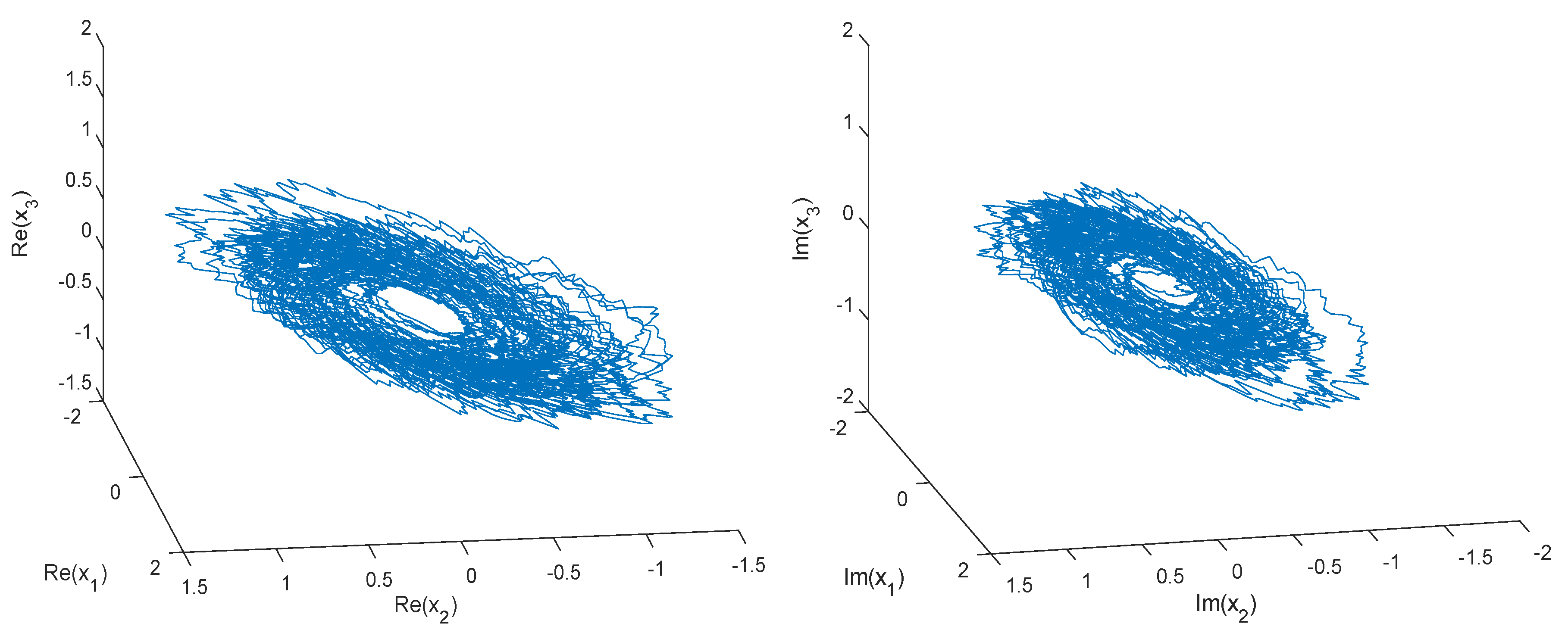
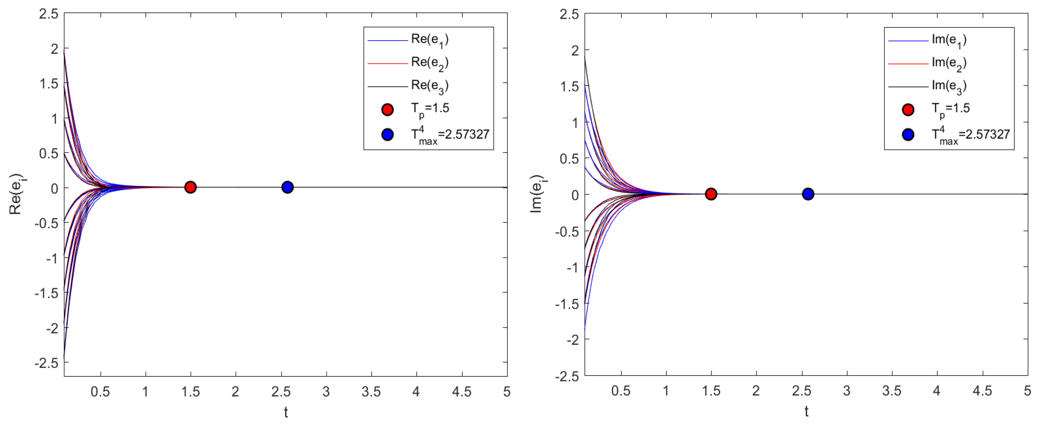
4. Numerical Results

In this section, we demonstrate the feasibility of the theoretical results of the previous section by numerical simulation with MATLAB 2023. The code used in this paper can be found in Appendix A.

Example 1.

For $\mathrm{m}=3$, consider the following CVSFCNNs with time delay:

$$\begin{array}{cc}\hfill d{x}_i\left(t\right)=[& -a_i{x}_i\left(t\right)+\sum _{\ell =1}^3{p}_{i\ell }{f}_{\ell }\left(x_{\ell }\left(t\right)\right)+\sum _{\ell =1}^3{b}_{i\ell }{f}_{\ell }\left(x_{\ell }(t-{\tau }_{\ell }\left(t\right))\right)+\sum _{\ell =1}^3{r}_{i\ell }{v}_{\ell }\hfill \\ \hfill & +\underset{\ell =1}{\overset{3}{\bigwedge }}{\alpha }_{i\ell }{f}_{\ell }\left(x_{\ell }(t-{\tau }_{\ell }\left(t\right))\right)+\underset{\ell =1}{\overset{3}{\bigwedge }}{T}_{i\ell }{v}_{\ell }+\underset{\ell =1}{\overset{3}{\bigvee }}{\beta }_{i\ell }{f}_{\ell }\left(x_{\ell }(t-{\tau }_{\ell }\left(t\right))\right)\hfill \\ \hfill & +\underset{\ell =1}{\overset{3}{\bigvee }}{S}_{i\ell }{v}_{\ell }+I_i]dt+{\sigma }_i\left(x_i\left(t\right),t\right)d\omega \left(t\right),\hfill \end{array}$$

(20)

where $f_1\left(u\right)=f_2\left(u\right)=f_3\left(u\right)=0.06\ast (tanh\left(Re\left(u\right)\right)+itanh\left(Im\left(u\right)\right))$. Other parameters of system (20) are as follows: $p_{11}=0.1+0.21i$, $p_{12}=-0.52+1.25i$, $p_{13}=1.52-1.4i$, $p_{21}=-0.45+3.15i$, $p_{22}=-0.42+0.16i$, $p_{23}=0.94-1.56i$, $p_{31}=-0.41+1.51i$, $p_{32}=-2.05+2.15i$, $p_{33}=1.55-1.96i$, $b_{11}=-0.4-0.75i$, $b_{12}=1.67+1.92i$, $b_{13}=2.07-1.72i$, $b_{21}=-1.08+5.15i$, $b_{22}=0.19+0.36i$, $b_{23}=1.31-1.36i$, $b_{31}=-1.04+1.51i$, $b_{32}=-1.48+3.15i$, $b_{33}=-0.35+0.81$, ${\alpha }_{11}=0.35+1.51i$, ${\alpha }_{12}=-1.69+0.1i$, ${\alpha }_{13}=0.3+0.16i$, ${\alpha }_{21}=-1.86+0.7i$, ${\alpha }_{22}=-0.62+0.36i$, ${\alpha }_{23}=0.21-1.32i$, ${\alpha }_{31}=0.1-0.26i$, ${\alpha }_{32}=-1.66+1.4i$, ${\alpha }_{33}=0.37-1.21i$, ${\beta }_{11}=0.67-1.92i$, ${\beta }_{12}=0.57-0.56i$, ${\beta }_{13}=0.78-0.61i$, ${\beta }_{21}=0.38-4.03i$, ${\beta }_{22}=0.97-1.48i$, ${\beta }_{23}=0.87-0.16i$, ${\beta }_{31}=0.25-0.46$, ${\beta }_{32}=0.64-0.19i$, ${\beta }_{33}=0.82-0.32i$, $a_1=1.68-0.9i$, $a_2=1.48-0.67i$, $a_3=1.54-0.45i$, and $I_i=1,{\sigma }_i=2+0.26i$ for $i=1,2,3$. The initial condition of system (20) is taken as $x_1\left(\theta \right)=0.6-0.3i,x_2\left(\theta \right)=-1.2+0.8i$, and $x_3\left(\theta \right)=-0.4+0.8i$. The MATLAB numerical simulation of system (20) under the above parameters is shown in Figure 1. It is not difficult to find that system (20) has a chaotic attractor.

The response system corresponding to CVSFCNNs (20) is:

$$\begin{array}{cc}\hfill d{y}_i\left(t\right)=[& -a_i{y}_i\left(t\right)+\sum _{\ell =1}^3{p}_{i\ell }{f}_{\ell }\left(y_{\ell }\left(t\right)\right)+\sum _{\ell =1}^3{b}_{i\ell }{f}_{\ell }\left(y_{\ell }(t-{\tau }_{\ell }\left(t\right))\right)+\sum _{\ell =1}^3{r}_{i\ell }{v}_{\ell }\hfill \\ \hfill & +\underset{\ell =1}{\overset{3}{\bigwedge }}{\alpha }_{i\ell }{f}_{\ell }\left(y_{\ell }(t-{\tau }_{\ell }\left(t\right))\right)+\underset{\ell =1}{\overset{3}{\bigwedge }}{T}_{i\ell }{v}_{\ell }+\underset{\ell =1}{\overset{3}{\bigvee }}{\beta }_{i\ell }{f}_{\ell }\left(y_{\ell }(t-{\tau }_{\ell }\left(t\right))\right)\hfill \\ \hfill & +\underset{\ell =1}{\overset{3}{\bigvee }}{S}_{i\ell }{v}_{\ell }+I_i+u_i\left(t\right)]dt+{\sigma }_i\left(y_i\left(t\right),t\right)d\omega \left(t\right),\hfill \end{array}$$

(21)

where $a_i,p_{i\ell },b_{i\ell },f_{\ell },{\alpha }_{i\ell },{\beta }_{i\ell },{\sigma }_i,$ and $I_i$ are defined as in system (20).

First, consider the FXT synchronization of the drive–response systems (20) and (21) under the controllers (4) and (15). Through simple calculation, we can obtain $L_i=1,{\eta }_i=2.8$. Therefore, the basic Assumption 1 is satisfied. By choosing $d_{11}=2.37$, $d_{12}=4.51$, $d_{13}=3.21,d_{21}=9.37$, $d_{22}=1.54,d_{23}=1.16$, $d_{31}=1.3,d_{32}=8.34$, $d_{33}=1.17,{\xi }_1=9.1$, ${\xi }_2=13.8,{\xi }_3=14.4$, ${\zeta }_1=7.1,{\zeta }_2=11.2$, ${\zeta }_3=12.7$, ${\theta }_1=1.4$, and ${\theta }_2=0.7$, it is not difficult to calculate $k=max\left\{k_i\right\}=10.1899$, and then the inequality (5) in Theorem 1 is also satisfied. Hence, according to Theorem 1, the drive–response systems (20) and (21) realize FXT synchronization in ST $T_{max}^3=1.8046$. The time evaluation of synchronization error between systems (20) and (21) is shown in Figure 2. For controller (15), if we choose $L_i=1,{\xi }_1=10.5,{\xi }_2=11.6,{\xi }_3=13.7,{\zeta }_1=6.1,{\zeta }_2=10.7,{\zeta }_3=11.9,{\theta }_1=1.3$, and ${\theta }_2=0.9$, then the drive–response systems (20) and (21) also realize FXT synchronization in ST $T_{max}^3=1.65202$. The time evaluation of synchronization error between systems (20) and (21) under controller (15) is shown in Figure 3.

Next, consider the PAT synchronization of systems (20) and (21) under controllers (18) and (19). Choosing $T_p=1.5,{\theta }_1=1.1$, and ${\theta }_2=0.9$, inequality (5) is also satisfied. Hence, according to Theorem 2, the drive–response systems (20) and (21) realize PAT synchronization at $T_p=1.5$. The time evaluation of synchronization errors between systems (20) and (21) is shown in Figure 4. It is not difficult to see that when ${\theta }_1+{\theta }_2=2$, the system achieves synchronization within the predefined time $T_p=1.5$, which is even smaller than the fixed-time $T_{max}^4=2.57327$. For controller (19), if we choose $T_p=1.2,{\theta }_1=1.1$, and ${\theta }_2=0.9$, then the drive–response systems (20) and (21) realize PAT synchronization at $T_p=1.2$. Figure 5 shows the time evaluation of synchronization error between systems (20) and (21) under controller (19). It is not difficult to see from Figure 5 that when ${\theta }_1+{\theta }_2=2$, the system achieves synchronization within the predefined time $T_p=1.2$, which is even smaller than the fixed-time $T_{max}^4=1.43329$.

Remark 6.

In the above Example, since FXT/PAT synchronization is not affected by the system’s initial condition and controller parameters, parameter values can be randomly selected as needed to meet the conditions of the theorem. Therefore, in this example, we first select specific parameter values as initial values based on previous research or literature. Then, through repeated experiments and optimization, these parameter values are adjusted to achieve the best simulation effect.

Remark 7.

By comparing Figure 1 and Figure 2, Figure 3, Figure 4 and Figure 5, it can be seen that, without a controller, the system will not reach a synchronous state (as shown in Figure 1, which presents a chaotic state). However, after adding a controller, the drive–response system reaches the same state after a period of time (see Figure 2, Figure 3 and Figure 4). Therefore, the controller designed in this article plays an important role in achieving FXT/PAT synchronization.

Remark 8.

In [41], Pang et al. realized the FXT synchronization of CVNNs in FXT $T_{max}=2.7662$ by designing a controller without the sign function; however, the controller designed in [41] consists of a linear term and three nonlinear terms. In this article, by removing the linear term, we construct controller (15), which is composed of only three nonlinear terms without the sign function, and which realizes the FXT synchronization of the studied system within $T_{max}^3=1.65202$ (see Figure 3). Obviously, the convergence time obtained in this article is much faster than [41]. Therefore, the controller constructed in this paper has more advantages than [41].

Remark 9.

The solid blue and red circles in the numerical figures represent time intervals during which the system achieves synchronization. For example, from Figure 2 and Figure 3, it can be observed that the system achieves synchronization within $T_{max}^3$. From Figure 4 and Figure 5, it can be inferred that the system achieves synchronization within a specified time interval $T_p$. In particular, it can be seen that when ${\theta }_1+{\theta }_2=2$, $T_p$ is smaller than $T_{max}^4$ (see Figure 4 and Figure 5). This representation allows us to easily determine whether the system achieves synchronization within a certain time interval and identify the specific time periods of synchronization.

5. Conclusions and Prospect

This paper investigates the synchronization problem of CVSFCNNs with time delays and adopts a non-separation approach for the study. Unlike previous research [14,15,32,40,41], the constructed controllers in these studies do not include the sign function, thus effectively avoiding the occurrence of chattering phenomena. Through theoretical analysis and system simulation, the effectiveness and superiority of the non-separable control method are validated. Experimental results demonstrate that our proposed approach achieves faster synchronization time compared to previous studies [41]. Therefore, this research provides a novel method for addressing the synchronization problem of CVFNNs with time delays, with significant theoretical and practical implications.

Prospect: In practical production and in life, many problems require processing higher-dimensional data, not limited to 2D or 3D. For example, fields such as autonomous driving, color image classification and forensics, and human motion recognition require processing of four-dimensional or higher-dimensional data. Therefore, we need to explore how to use four-dimensional or higher-dimensional data to solve these problems. This may involve the development of new mathematical models and algorithms, as well as the expansion and improvement of existing technologies. By studying and exploring these new research directions, we can better solve practical problems and promote the development of mathematics and neural networks. Therefore, in the future, we will focus on researching how to process and analyze four-dimensional or higher-dimensional data to solve practical production and life problems.

References

1. Chua, L.; Yang, L. Cellular Neural Networks: Theory. IEEE Trans. Circuits Syst. 1988, 35, 1257–1272. [Google Scholar] [CrossRef]
2. Chua, L.; Yang, L. Cellular Neural Networks: Applications. IEEE Trans. Circuits Syst. 1988, 35, 1273–1290. [Google Scholar] [CrossRef]
3. Klaus, M. Cellular neural networks and visual computing. Int. J. Bifurc. Chaos 2003, 13, 1–6. [Google Scholar]
4. Duan, S.; Hu, X.; Wang, L.; Gao, S.; Li, C. Hybrid memristor/RTD structure-based cellular neural networks with applications in image processing. Neural Comput. Appl. 2013, 25, 291–296. [Google Scholar] [CrossRef]
5. Yang, T.; Yang, L.; Wan, C.; Chua, L. Fuzzy Cellular Neural Networks: Theory. In Proceeding of the 1996 Fourth IEEE international workshop on cellular neural networks and their applications proceedings (CNNA-96), Seville, Spain, 24–26 June 1996; IEEE: Piscataway, NJ, USA, 1996; pp. 181–186. [Google Scholar]
6. Yao, X.; Liu, X.; Zhong, S. Exponential stability and synchronization of Memristor-based fractional-order fuzzy cellular neural networks with multiple delays. Neurocomputing 2021, 419, 239–250. [Google Scholar] [CrossRef]
7. Muhammadhaji, A.; Abdurahman, A. General decay synchronization for fuzzy cellular neural networks with time-varying delays. Int. J. Nonlinear Sci. Numer. Simul. 2019, 20, 551–560. [Google Scholar] [CrossRef]
8. Haider, K.; Ahmed, A. Fuzzy-cellular neural network for face recognition HCI Authentication. J. Phys. Conf. Ser. 2018, 1003, 012033. [Google Scholar]
9. Gang, Y. New results on the stability of fuzzy cellular neural networks with time-varying leakage delays. Neural Comput. Appl. 2014, 25, 1709–1715. [Google Scholar]
10. Ceylan, M.; Ceylan, R.; Kara, S. Application of complex discrete wavelet transform in classification of Doppler signals using complex-valued artificial neural network. Artif. Intell. Med. 2008, 44, 65–76. [Google Scholar] [CrossRef]
11. Valle, M. Complex-valued recurrent correlation neural networks. IEEE Trans. Neural Netw. Learn. Syst. 2014, 23, 1600–1612. [Google Scholar] [CrossRef]
12. Pande, A.; Thakur, A.K.; Roy, S. Complex-Valued Neural Network in Signal Processing: A Study on the Effectiveness of Complex Valued Generalized Mean Neuron Model. Proc. World Acad. Sci. Eng. Technol. 2008, 27, 240–245. [Google Scholar]
13. Hirose, A. Complex-Valued Neural Networks: Advances and Applications; John Wiley & Sons: Hoboken, NJ, USA, 2013. [Google Scholar] [CrossRef]
14. Guo, Y.; Luo, Y.; Wang, W.; Luo, X.; Ge, C.; Kurths, J.; Yuan, M.; Gao, Y. Fixed-time synchronization of complex-valued memristive BAM neural network and applications in image encryption and decryption. Int. J. Control Autom. Syst. 2019, 18, 462–476. [Google Scholar] [CrossRef]
15. Zhang, Z.; Guo, R.; Liu, X.; Zhong, M.; Lin, C.; Chen, B. Fixed-time synchronization for complex-valued BAM neural networks with time delays. Asian J. Control 2019, 23, 298–314. [Google Scholar] [CrossRef]
16. Feng, L.; Yu, J.; Hu, C.; Yang, C.; Jiang, H. Nonseparation method-based finite/fixed-time synchronization of fully complex-valued discontinuous neural networks. IEEE Trans. Cybern. 2021, 51, 3212–3223. [Google Scholar] [CrossRef]
17. Xiong, K.; Yu, J.; Hu, C.; Jiang, H. Synchronization in finite/fixed time of fully complex-valued dynamical networks via nonseparation approach. J. Frankl. Inst. 2020, 357, 473–493. [Google Scholar] [CrossRef]
18. Shirke, D.; Raja, C. Optimization driven deep belief network using chronological monarch butterfly optimization for iris recognition at-a-distance. Int. J. Knowl.-Based Intell. Eng. Syst. 2022, 26, 17–35. [Google Scholar] [CrossRef]
19. Ramezanpanah, Z.; Mallem, M.; Davesne, F. Autonomous gesture recognition using multi-layer LSTM networks and laban movement analysis. Int. J. Knowl.-Based Intell. Eng. Syst. 2023, 26, 1–9. [Google Scholar] [CrossRef]
20. Giebel, S.; Rainer, M. Stochastic processes adapted by neural networks with application to climate, energy, and finance. Appl. Math. Comput. 2011, 218, 1003–1007. [Google Scholar] [CrossRef]
21. Shi, Y.; Zhu, P. Finite-time synchronization of stochastic memristor-based delayed neural networks. Neural Comput. Appl. 2016, 29, 293–301. [Google Scholar] [CrossRef]
22. Liu, M.; Wu, H. Stochastic finite-time synchronization for discontinuous semi-Markovian switching neural networks with time delays and noise disturbance. Neurocomputing 2018, 310, 246–264. [Google Scholar] [CrossRef]
23. Zhang, W.; Yang, X.; Li, C. Fixed-time stochastic synchronization of complex networks via continuous control. IEEE Trans. Cybern. 2019, 49, 3099–3104. [Google Scholar] [CrossRef] [PubMed]
24. Xu, Y.; Wu, X.; Mao, B.; Lu, J.; Xie, C. Fixed-time synchronization in the pth moment for time-varying delay stochastic multilayer networks. IEEE Trans. Syst. Man Cybern. Syst. 2020, 52, 1135–1144. [Google Scholar] [CrossRef]
25. Wang, L.; Zhang, C. Exponential Synchronization of Memristor-Based Competitive Neural Networks With Reaction-Diffusions and Infinite Distributed Delays. IEEE Trans. Neural Netw. Learn. Syst. 2022, 1–14. [Google Scholar] [CrossRef] [PubMed]
26. Wang, L.; He, H.; Zeng, Z. Global Synchronization of Fuzzy Memristive Neural Networks with Discrete and Distributed Delays. IEEE Trans. Fuzzy Syst. 2019, 28, 2022–2034. [Google Scholar] [CrossRef]
27. Polyakov, A. Nonlinear feedback design for fixed-time stabilization of linear control systems. IEEE Trans. Autom. Control 2012, 57, 2106–2110. [Google Scholar] [CrossRef]
28. Feng, L.; Hu, C.; Yu, J.; Jiang, H.; Wen, S. Fixed-time Synchronization of Coupled Memristive Complex-valued Neural Networks. Chaos Solitons Fractals 2021, 148, 110993. [Google Scholar] [CrossRef]
29. Wang, S.; Zhang, Z.; Lin, C.; Chen, J. Fixed-time synchronization for complex-valued BAM neural networks with time-varying delays via pinning control and adaptive pinning control. Chaos Solitons Fractals 2021, 153, 111583. [Google Scholar] [CrossRef]
30. Hu, C.; He, H.; Jiang, H. Fixed/Preassigned-Time Synchronization of Complex Networks via Improving Fixed-Time Stability. IEEE Trans. Cybern. 2020, 51, 2882–2892. [Google Scholar] [CrossRef]
31. You, J.; Abdurahman, A.; Sadik, H. Fixed/predefined-time synchronization of complex-valued stochastic BAM neural networks with stabilizing and destabilizing impulse. Mathematics 2022, 10, 4384. [Google Scholar] [CrossRef]
32. Li, X.; Zhang, W.; Fang, J.; Li, H. Event-triggered exponential synchronization for complex-valued memristive neural networks with time-varying delays. IEEE Trans. Neural Netw. Learn. Syst. 2020, 31, 4104–4116. [Google Scholar] [CrossRef]
33. Zadeh, L.A. Fuzzy Sets. Inf. Control 1965, 8, 338–353. [Google Scholar] [CrossRef]
34. Cui, W.; Wang, Z.; Jin, W. Fixed-time synchronization of Markovian jump fuzzy cellular neural networks with stochastic disturbance and time-varying delays. Fuzzy Sets Syst. 2021, 411, 68–84. [Google Scholar] [CrossRef]
35. Abudusaimaiti, M.; Abdurahman, A.; Jiang, H.; Hu, C. Fixed/predefined-time synchronization of fuzzy neural networks with stochastic perturbations. Chaos Solitons Fractals 2022, 154, 111596. [Google Scholar] [CrossRef]
36. Chen, S.; Li, H.; Kao, Y.; Zhang, L.; Hu, C. Finite-time stabilization of fractional-order fuzzy quaternion-valued BAM neural networks via direct quaternion approach. J. Frankl. Inst. 2021, 358, 7650–7673. [Google Scholar] [CrossRef]
37. Zhang, Y.; Zhuang, J.; Xia, Y.; Bai, Y.; Cao, J.; Gu, L. Fixed-time synchronization of the impulsive memristor-based neural networks. Commun. Nonlinear Sci. Numer. Simul. 2019, 77, 40–53. [Google Scholar] [CrossRef]
38. Akyol, K. Comparing of deep neural networks and extreme learning machines based on growing and pruning approach. Expert Syst. Appl. 2020, 140, 112875. [Google Scholar] [CrossRef]
39. Deng, H.; Bao, H. Fixed-time synchronization of quaternion-valued neural networks. Phys. A Stat. Mech. Its Appl. 2019, 527, 121351. [Google Scholar] [CrossRef]
40. Zhang, J.; Ma, X.; Li, Y.; Gan, Q.; Wang, C. Synchronization in fixed/preassigned-time of delayed fully quaternion-valued memristive neural networks via non-separation method. Commun. Nonlinear Sci. Numer. Simul. 2022, 113, 106581. [Google Scholar] [CrossRef]
41. Pang, M.; Zhang, Z.; Wang, X.; Wang, Z.; Lin, C. Fixed/preassigned-time synchronization of high-dimension-valued fuzzy neural networks with time-varying delays via nonseparation approach. Knowl.-Based Syst. 2022, 255, 109774. [Google Scholar] [CrossRef]
Figure 1. The chaotic attractor of real and imaginary parts of system (20).
Mathematics 11 03769 g001
Figure 2. Evaluation of real and imaginary parts of synchronization errors under controller (4) with ( θ 1 , θ 2 ) = ( 1.4 , 0.7 ) .
Mathematics 11 03769 g002
Figure 3. Evaluation of real and imaginary parts of synchronization errors under controller (15) with ( θ 1 , θ 2 ) = ( 1.3 , 0.9 ) .
Mathematics 11 03769 g003
Figure 4. Evaluation of real and imaginary parts of synchronization errors under controller (18) with ( θ 1 , θ 2 ) = ( 1.1 , 0.9 ) .
Mathematics 11 03769 g004
Figure 5. Evaluation of real and imaginary parts of synchronization errors under controller (19) with ( θ 1 , θ 2 ) = ( 1.1 , 0.9 ) .
Mathematics 11 03769 g005
Disclaimer/Publisher’s Note: The statements, opinions and data contained in all publications are solely those of the individual author(s) and contributor(s) and not of MDPI and/or the editor(s). MDPI and/or the editor(s) disclaim responsibility for any injury to people or property resulting from any ideas, methods, instructions or products referred to in the content.