Article

Assessing the Compatibility of Railway Station Layouts and Mixed Heterogeneous Traffic Patterns by Optimization-Based Capacity Estimation

1
State Key Laboratory of Advanced Rail Autonomous Operation, Beijing Jiaotong University, Beijing 100044, China
2
China Railway Design Corporation, Tianjin 300142, China
*
Author to whom correspondence should be addressed.
Mathematics 2023, 11(17), 3727; https://doi.org/10.3390/math11173727
Submission received: 1 August 2023 / Revised: 28 August 2023 / Accepted: 28 August 2023 / Published: 30 August 2023

Abstract

:
The operations performance of a railway station depends on the compatibility of its layout and the traffic pattern. It is necessary to determining an adaptable station layout for a railway station in accordance with its complex traffic pattern during the design phase. This paper assesses the railway station layout from a capacity perspective. In particular, this paper addresses an optimization-based capacity estimation approach for the layout variants of a railway station (i.e., the number of siding tracks and the structure of the connections in between) considering the traffic pattern variants. A mixed integer programming model for microscopic timetable compression is applied to calculate the occupation rate of the given traffic pattern with flexible route choices and train orders. A novel “schedule-and-fix” heuristic algorithm is proposed to solve large-scale instances efficiently. In the case study, we evaluate the performance of the schedule-and-fix method compared with the benchmark solvers Gurobi and CP-SAT. Applying the proposed method, we compare the capacity performances of the two station design schemes, i.e., one with a flyover and the other without. The result shows that, for the given instance, building a flyover gains capacity benefits as it reduces the potential conflict in the throat area. However, the level of benefit depends on the combination of trains. It is necessary to build the flyover when the proportion of turn-around trains is more than 70% from the perspective of station capacity.

1. Introduction

1.1. The Compatibility of Station Layouts and Traffic Patterns

The continuous growth of infrastructure investment in developing countries plays a significant role in their economic growth. Railway is a rapid, sustainable, and long-distance transportation system, attracting much attention in the field of infrastructure investment. Similar to typical infrastructure investments, railway infrastructure investments are costly and require extensive research on the designs in the planning phases. Railway stations have sophisticated layouts for operating complex and time-consuming train movements; thus the layout have significant impacts on the performance of the station, e.g., the number of tracks next to passenger platforms, the connection between station tracks, the length of the track used, and the connectivity between the tracks and the adjacent segments.
For improving the operation efficiency of stations, the layouts should be properly designed according to the traffic patterns (i.e., the combinations of various types of trains). This task is particularly challenging when the traffic pattern in the station is complex. For stations connecting more than one railway line, trains running towards different directions are scheduled within the same time slot. These trains might have temporal and spatial conflicts which prevent them being operated simultaneously and reduce the operation performance. An optimized layout design of the station can resolve the conflicts to a large extent by setting up flexible connection between the siding tracks and the open track sections to increase the capacity of the station. Therefore, analyzing the compatibility of the station layout and the traffic pattern is the key step for evaluating the design of the station layout.
An essential evaluation metric of the station layout from the operation perspective is the station capacity. Station capacity, defined as the maximum number of trains that can arrive at/depart from the station in a specific time interval [1], is an essential performance index justifying if the design scheme satisfies the predicted traffic demand (i.e., the required number of trains operated in the station). Various factors determine station capacity, including the number of siding tracks and the signal system’s performance. Furthermore, the connection between siding tracks to open track segments significantly impacts the station capacity as well. However, the well-designed connections resolve the potential conflicts of train movements and therefore improve the capacity. For example, building a flyover at the throat area (i.e., the area with many switches connecting the open track segments and siding tracks) can resolve the conflict between the arrival and departure operation, therefore increasing the station capacity. As shown in Figure 1, the layout shown in Figure 1b with a flyover avoids the arrival and departure conflicts shown in Figure 1a. Therefore, a higher capacity can be achieved.
However, the construction of a flyover is a costly project. The land acquisition and demolition for land utilization require a considerable budget. The design, building, and maintenance of the flyover also need a long-term financial outlay from the railway infrastructure manager. Furthermore, many issues concerning land use planning, such as environmental impact assessment (EIA) and public welfare evaluation, should be carefully investigated to maximize the profit of constructing the railway station. For example, it would be uneconomical to use the layout of Figure 1b instead of Figure 1a if the potential conflicts were infrequent, since the capacity improvement from flyover construction is not fully utilized in practice. Therefore, capacity estimation of stations is necessary to determine the station performance applying particular layouts. The compatibility of the station layout design and its traffic pattern, which impacts the efficiency of the infrastructure investment, is determined by the performance under specific traffic patterns.
The accuracy of the capacity estimation is determined by the infrastructure and train movement modeling, the applied operation parameters, and the solution algorithm. In this paper, we apply a timetable compression method for estimating the station capacity. Specifically, based on the initially designed timetable with specific traffic patterns, we apply a mathematical model to compress the timetable and calculate the makespan (i.e., the shortest time for finishing all train operations), which implicitly tells the maximum number of scheduled trains with such traffic patterns in a certain period. The capacity estimation method proposed in this paper helps estimate the station performance under complicated mixed train traffic and decide the best capacity improvement measures. The level of the station capacity improvement from building a flyover can be quantitively estimated by this proposed method. The result can be used to determine if a station layout is worth building from the aspect of train traffic management.
The remainder of the paper is organized as follows. Section 1.2 summarizes the literature associated with the railway station capacity estimation, followed by the contribution statements of this paper in Section 1.3. Section 2 describes the modeling of the railway station infrastructure, train movements, and the occupation rules of the resources. Based on the description of Section 2, Section 3 proposes a mixed integer programming model and corresponding solution method for timetable compression, considering the flexible route choices and train orders. One can compute the occupation rate of the derived compressed timetable to estimate the railway capacity under certain mixed traffic combinations. Section 4 provides the results and discussions of a series of case studies displaying the performance of the solution method and showing the variation of the station capacity applying different design schemes, train combinations, as well as operational parameters. The applied methodology and the central finding of this paper are concluded in Section 5.

1.2. Literature Review of Station Capacity Estimation

Railway infrastructure capacity is typically defined as the total number of possible paths in a defined time window, considering the actual path mix or known developments, respectively, and the IM (infrastructure manager)’s assumptions about nodes, individual lines, or parts of the network with respect to market-oriented quality [1]. As part of the railway infrastructure, the railway station inherits the capacity concept, which can be derived as the maximum number of scheduled trains operated in the station within a defined time window with given train combinations and other extra operation requirements. Khadem-Sameni et al. [2] introduce the problems and the current challenges of railway capacity in Britain.

Capacity Estimation Methods

Typical capacity estimation methods for railway stations include analytical, simulation, timetable compression, and optimization methods.
(1)
Analytical method
Analytical methods use mathematical formulations to calculate the station capacity with some input information directly. In general, the input of the analytical method is less than in the timetable-related method, which enables the method to be applied in the infrastructure design phase when detailed data is missing. However, the accuracy of the result derived from the analytical method depends on the parameters. Malavasi et al. [3] analyze three classical analytical methods for station capacity estimation, namely the Potthoff method, Probabilistic method, and Deutsche Bahn method, and compare the computational results of the three methods in two stations. Wang et al. [4] provide a capacity enhancement measurement by transforming the existing fixed train-approaching locking section into a variable mode. An analytical formulation for calculating the theoretical capacity is applied to estimate the level of capacity enhancement. Veselý [5] proposes an analytical method for calculating the railway station capacity.
Some research applies queueing theory for modeling the stochastic procedures of the operation within stations. Bychkov et al. [6] apply a queuing network to describe the operation of railway stations. The yards of a railway station are modeled as nodes of a queuing network, and the train operations are modeled as flows in the network. A simulation approach is applied to solve the model. Yuan and Hansen [7] estimate the knock-on delays of trains caused by route conflicts and late transfer connections by a stochastic analytical model. The model is applied for optimizing the station capacity utilization of The Hague Holland Spoor by setting an appropriately scheduled buffer time. Corriere et al. [8] investigate the impact of reliability on station capacity and propose a logic fuzzy model to estimate the theoretical station capacity considering the frequency of accidents.
(2)
Simulation method
Microscopic simulation is commonly used for estimating the station capacity, especially when the uncertainty of train operation is considered. Han et al. [9] present a railway station Infrastructures Representing Model (IRM) for fixed equipment. An analytical method based on the occupation time of switch groups and tracks is applied to compute the overall station capacity. Furthermore, a microscopic simulation method is also applied to estimate the capacity of a passenger station. Zhong et al. [10] use a mesoscopic simulation method for analyzing and calculating the carrying capacity of railway passenger stations, where the arrival time distribution of trains is considered in the generation of train movements. Bulíček et al. [11] propose an idea to increase the station capacity by adding a switch point area. They use an analytical and a mesoscopic simultaneous stochastic simulation model to verify the effectiveness of the capacity increment measurement. Three infrastructure variants are evaluated. The microscopic simulation method can describe and perform the station operations in a very detailed manner, but it requires sophisticated input data (e.g., track layout, parameters of the signaling system, and train timetable), which limit its implementation in the infrastructure designing phase.
(3)
Data-driven approaches
The realistic historical operation data of stations can be used for analyzing the practical capacity utilization. The train delay and the occupation rate of track circuits and platforms can reveal the bottleneck of the station capacity. Armstrong and Preston [12] study the relationship between capacity provision (utilization) and service quality using a data-driven method. Historic timetables and delay data are used to investigate the relationships to determine an appropriate station capacity utilization level. Yuan and Hansen [13] conducted an empirical investigation based on historical data to estimate the station capacity utilization of the Hague HS station. They concluded that the buffer times between trains and their distribution affect the propagation of train delays.
(4)
Extended UIC Code 406 timetable compression method
The timetable compression method is a well-known capacity estimation method mentioned and recommended by the UIC code 406 leaflet. The station capacity is denoted by the capacity occupation rate of a compressed timetable, where the slack times between trains are removed as much as possible. The original UIC Code 406 timetable compression method is used to determine the capacity of railway sections on a macroscopic level. Necessary modifications, including the topology description of the station, the train movement description, and the resource occupation rules, are required when applying the method on stations (typically microscopic level). Landex [14] uses a series of capacity estimation methods, i.e., an adapted UIC 406 capacity method, an analytical method, and an optimization method for analyzing and improving the station capacity. These methods consider the probability of conflicts and train arrival delays. Johansson and Weik [15] proposed a UIC 406-based method at the station level for long-term infrastructure planning. The method is timetable-independent as the workflow consists of a pattern train generation and a timetable generation procedure. Zhong et al. [16] compare a combination–reconstruction (ComRec) method, a triangular-gap-problem method, and a max-plus algebra method for generating compressed timetables and show that these three methods are equivalent. Kavička et al. [17] apply the software tool MesoRail based on the UIC 406 method to calculate the occupation rate of railway stations. Lindner [18] analyzes the problem when applying the UIC 406 method and concludes that the UIC 406 compression method can only offer significant results if the user evaluates an infrastructure that ensures conflict-free station areas. Gašparík [19] developed a conceptual framework for an easier evaluation of occupation time in the train traffic diagram based on UIC 406.
Note that in the UIC Code 406 leaflet [1] and its updated version [20], the adaptability of the timetable compression method applied to the station is not discussed and verified. Many issues must be tackled when applying the timetable compression method at the station level, such as the train route choice, the train order determination, and the occupancy rules of track circuits.
(5)
Optimization approach
Optimization approaches build mathematical programming models to directly solve the station capacity, which can be categorized into timetable-independent and timetable-dependent methods based on the role of timetables.
Timetable-independent optimization approaches describe railway traffic in a macroscopic manner, neglecting details of traffic patterns on timetables. The capacity estimation results are regarded as “absolution capacity” or “theoretical capacity”. These methods are useful in the infrastructure planning phase when the traffic pattern of the station is not determined. Sameni et al. [21] apply a DEA method to investigate the technical efficiency and service effectiveness of railway stations. Various impact factors, including the number of platforms, the fraction of through lines, and the number of trains with scheduled stops, are ranked according to their contribution to the evaluation indices. Jovanović et al. [22] propose a two-stage optimization approach to estimate the theoretical capacity without predetermined timetables, where the first stage determines the compatible route sets, and the second stage determines the optimum sequence of the route sets. The conflicts of routes are described as a graph coloring problem, and the total follow-up time is minimized by a traveling salesman problem.
Timetable-dependent optimization approaches often conduct timetable saturation, i.e., schedule a fully saturated timetable using the trains from a given train pool. The station capacity is then regarded as the total number of scheduled trains in the saturated timetable. Ignatov and Naumov [23] apply an MIP model to insert additional trains to a basic timetable considering random delays for increasing railway station capacity. Sels et al. [24] propose an optimum track allocation problem for trains to estimate the station capacity. It considers the actual, current, as well as future train set scenarios with increasing traffic. The module is fully integrated with the software named Infrabel. Guo et al. [25] solve the station carrying capacity problem and consider train set utilization constraints. The minimum turn-around time of trains, the capacity of vehicle depots, as well as the entering and exiting procedure, are considered. Dollevoet et al. [26] include the capacities (i.e., the platform assignment) of the stations when developing a train delay management model. Javadian et al. [27] develop an optimization formulation and a simulated annealing algorithm to determine the capacity of rail yards.
The above methods are compared in Table 1.
In the above research, the capacity estimation in the stations with complex structures is considered difficult. The analytical method has unknown parameters for describing the capacity loss due to the traffic pattern, which is difficult to calibrate. These parameters also vary from station to station. The improved UIC 406 methods can only investigate the station capacity with a certain traffic pattern and are not able to explore the impact of different traffic patterns on the capacity variation. The timetable saturation methods have solution efficiency issues and are difficult to apply in large-scale problems, especially for those with heavy traffic. These drawbacks limit the application of the station capacity estimation method in realistic railway station design tasks.

1.3. Contribution Statements

To our knowledge, although many studies investigate the station capacity estimation problem differently, there is still a knowledge gap between the theory and the practice. In particular, train timetable compression methods considering flexible track assignments, route choices, and train operation orders are significantly less, as modeling the complex train movements with multiple stages (i.e., shunting, arrival, departure, and turn-around in between) and the corresponding resource occupations are difficult. Furthermore, the effective solution methods for solving the large-scale capacity estimation optimization model are still in shortage and need further development.
Therefore, we propose a mixed integer programming model and an associated solution algorithm to compress the given timetable while allowing flexible route choice and train order modification. The contributions of this paper are as follows.
  • A mixed integer programming model is proposed for estimating the station capacity considering the heterogeneous traffic within the station for infrastructure construction decision-making purposes. The model considers flexible route choices and train orders of occupying track circuits at a microscopic level, where the train operations with the uncertain number of multiple movements can be described.
  • A novel “schedule-and-fix” heuristic approach for solving large-scale problems is applied. Compared with MIP solver Gurobi and CP-SAT, the proposed heuristic can obtain feasible solutions very effectively with remarkable qualities.
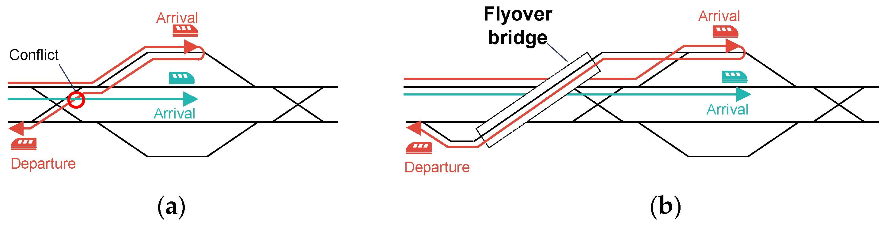
  • From a capacity perspective, this research investigates two typical station layouts (i.e., with or without flyover for departure trains). The flyover is considered necessary to build when the proportion of turn-around trains exceeds 70%. The capacity improvement difference of building a flyover by various train combinations and operation parameters is evaluated.
In general, our proposed timetable-based station capacity estimation method can overcome the drawback of the UIC 406 method to investigate the station capacity with flexible route choices and train sequences. The proposed heuristic method shows the potential of solving the large-scale problem in an acceptable short time, which enables the application of the method in the station design task.

2. Modeling the Microscopic Train Operation for Stations

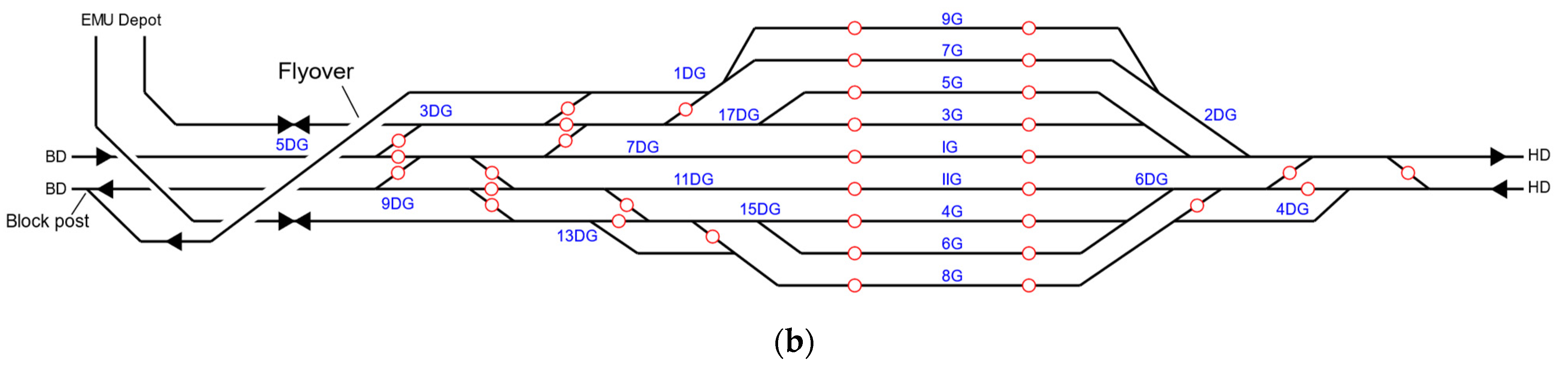
2.1. Modeling the Station Layout and Signal Facilities

2.1.1. Rail Sections within a Station

A railway station consists of many branching rail sections, which allow trains to drive between the borders of the station and their dwelling tracks. In order to describe the routes that train traverses, we need to build the topological model of the rail sections within stations. Four types of equipment can split rails into sections, including home signals, departure signals, switches, and insulation joints. The splitting of the rail sections within a station can be referred to in Figure 2.
The entire layout of a station can be described as an undirected network G ( N , L ) , where N is the node set, and L is the link set. A rail section can be regarded as an undirected link of the network, denoted by l L . A splitter can be regarded as a node of the network, denoted by n N .

2.1.2. Cells within a Station

Rail sections are clustered into cells according to the track circuit design of the interlocking system. A cell is denoted by c , and the cell set of the entire station is C , where c C . The link set L c includes the rail sections that belong to cell c . For example, in Figure 2, the rail sections in the red dashed rectangle form a cell, as they belong to the same track circuit. Note that according to the principle of interlocking system design, a rail section can and can only belong to one cell, namely c C L c = .
According to the working mechanism of the interlocking system, a cell can be used by at most one train at a specific moment. Therefore, the concept of “cell” plays a critical role in detecting and resolving the conflict of train traffic in a station.

2.2. Heterogeneous Train Movement Modeling

We assume that a train cannot be separated in the station. A train can only enter from a border node and leave the station at the other border node. In between, the train can only stop at the siding track for a duration. In other words, a train cannot stop at any rail section except for the siding track.

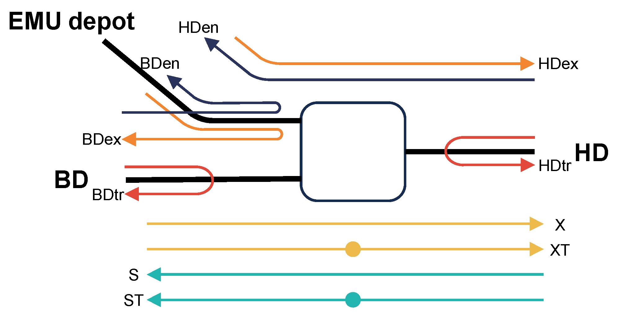
2.2.1. Train Arrival, Departure, and Dwell Movements

Only three types of train movements can happen in stations, namely arrival, departure, and dwell movement, as shown in Figure 3. We use e to denote a train movement and use three movement sets, namely E A , E D , and E W to include all arrival, departure, and dwell movements separately. Each movement has its beginning and ending time, which can be represented by a m and d m , respectively.
  • Arrival movement: An arrival movement implies that the train enters from the corresponding arrival border of the station and runs towards a siding track.
  • Departure movement: A departure movement implies that the train leaves from the siding track and runs towards the border node for its departure.
  • Dwell movement: Although no displacement of the train happens when a train dwells at the siding track, we still propose a unique movement to describe the train dwelling for unification purposes. A dwell movement denotes the train stop at a siding track for a specific duration. Note that if the train passes through the station without stopping, the dwell movement can be regarded as a dummy movement with a 0-time duration.
The movement chain with multiple arrival, departure, and dwell movements can describe the heterogeneous train traffic within different directions and train types, as well as the route choice within the station.

2.2.2. Route Assignment of the Movements

Each movement must be assigned an associated train route to finish its physical displacement. For each movement m , we generate the possible train route set R m according to the starting and ending point matching, the operation facility requirements (e.g., the train with boarding and alighting operation must select a dwell route with a platform), and other conditions.
For train route set generation, we propose a tag-matching method. On the one hand, the route matching tag 𝓉 is a descriptive string. For example, if a dwell route can only serve short coupling trains because of the length limitation, it would be marked “SHORT” as a tag. For train route r , we define a route-matching tag set T r in which the descriptive pattern of the route is included. On the other hand, for train movement m , we define an allow route matching tag set T m a l l o w and a deny route matching tag set T m d e n y . The movement m is possible to select the train route r only when all allow matching tags in T m a l l o w are in T r , and no deny matching tag in T m d e n y is in T r at the same time. Therefore, we can generate the train candidate route set R m by the following formulation.
R m = r R T m allow T r T r T m deny =

2.3. Cell Occupation Rules of Movements

A train movement m occupies a series of track circuits included in the cell set C m in a predetermined sequence. The cell set C m is generated by the following formulation.
C m = c C r | r R m
Note that only the cells on the selected route are occupied. The starting and ending occupation time of a cell by a movement is determined by the working principle and the performance of the interlocking system, as well as the train length and dynamic performance.
In this paper, we assume the station applies a so-called “route-lock-section-release” interlocking mechanism (Lu et al. [28]). Under this principle, all corresponding cells begin to be occupied simultaneously once the route is established. However, the cells are released (occupation ends) once the train leaves. In other words, the cells occupied by a movement are released one after another by a specific sequence. The detailed parameter estimation method can be referred to in Hansen and Pachl [29]. Based on the working principle of the interlocking system, the preoccupation and release time of the track circuit can be calculated according to the operation procedure of interlocking systems, the length of tracks, the breaking distance, and the velocity of trains. The concrete preoccupation and release time of different movements can be calculated. In this paper, we assume that the length and the arrival and departure velocity of trains are known, which means that we can calculate the relative time of the starting and ending time of cell occupation with the beginning and ending time of the movement. Therefore, analytical or simulation methods can estimate the cell occupation time.
Note that the passing through (without stopping) movement is regarded as a special dwell movement, i.e., the dwell movement with 0 dwell duration. A passing-through train’s arrival and departure speeds are significantly different from the train with stoppings. Furthermore, the station route establishment procedure is also different (For the train passing through without stopping, the arrival and departure routes are simultaneously established).

3. Timetable Compression Model for Station Capacity Estimation

3.1. Mathematical Model for Timetable Compression

We propose a combinatorial optimization model to compress a timetable for the capacity estimation purpose. Specifically, we build a mixed integer programming model minimizing the makespan of the timetable, subject to the train route selection, movement duration, cell occupancy constraints, as well as other side constraints. The notations used in the mathematical programming are listed in Table 2 and Table 3.
The objective function is to minimize the summation of the finishing time d m of all movements. This objective implies that the optimum solution ensures a “compressed” station train schedule with the minimum makespan.
Model 1
min f F   m M f   d m
Subject to:
(1) Movement duration constraint
d m a m δ m m i n f F , m M f
d m a m δ m m a x f F , m M f
(2) Train conservation constraint
d m = a g ( m ) f F , m M f , g m m n u l l
(3) Train route connection constraint
r 2 R g m   1 η r 1 , r 2 × x g m , r 2 + 1 x m , r 1 × Q 0 f F , m M f , g m m n u l l , r 1 R m
r 2 R g m   1 η r 1 , r 2 × x g m , r 2 1 x m , r 1 × Q f F , m M f , g m m n u l l , r 1 R m
(4) Movement time window constraint
d m ¯ l m d e p d m d m ¯ + h m d e p f F , m M f
a m ¯ l m a r r a m a m ¯ + h m a r r f F , m M f
(5) Route selection constraint
r R m   x m , r = 1 f F , m M f
(6) Cell occupation time constraint
s m , c + Q × 1 x m , r a m + θ r , c f F , m M f , r R m , c C r
s m , c a + θ r , c + Q × 1 x m , r f F , m M f , r R m , c C r
e m , c + Q × 1 x m , r d + β r , c f F , m M f , r R m , c C r
e m , c d + β r , c + Q × 1 x m , r f F , m M f , r R m , c C r
(7) Cell occupation conflict constraint
1 y c , m 1 , m 2 × Q + s m 2 , c e m 1 , c f 1 F , f 2 F f 1 , m 1 M f 1 , m 2 M f 2 , c C m 1 C m 2
y c , m 1 , m 2 + y c , m 2 , m 1 = 1 f 1 F , f 2 F f 1 , m 1 M f 1 , m 2 M f 2 , c C m 1 C m 2
(8) Variable domain constraint
x m , r 0 , 1 f F , m M f , r R m
y c , m 1 , m 2 0 , 1 f 1 F , f 2 F f 1 , m 1 M f 1 , m 2 M f 2 , c C m 1 C m 2
a m , d m R f F , m M f
s m , c , e m , c R f F , m M f , c C m
The objective function of Formulation (3) is to minimize the total finishing time of all movements of the given train, implying that the timetable is compressed. Constraints (4) and (5) are movement duration constraints, indicating that the duration of a movement should be between a given min–max range. Constraint (6) is the train movement conservation constraint between two consecutive movements, implying that a movement’s beginning time is identical to its previous movement’s ending time. Constraint (7) and (8) are train route connection constraints, ensuring that the starting position of a movement is identical to the ending position of its previous movement. Constraint (9) and (10) ensure that a movement happens within a given time window. Constraint (11) is the route selection constraint, implying any movement can and can only choose one route to operate. Constraints (12) to (15) are used for cell occupation time calculation, specifying the cells’ starting and ending occupation time for each movement. Constraints (16) and (17) are the conflict avoidance constraints, making sure that the occupancy times of a cell are without overlapping. Constraints (18) to (21) are variable domain constraints.

3.2. Solution Method

The model is a complex mixed-integer programming model. In this study, we apply two MIP solvers, namely Gurobi and CP-SAT from Google OR-Tools, to obtain the solution performance benchmarks. Gurobi is a MILP solver that applies exact algorithms, including branch-and-bound, cutting plane, etc., while CP-SAT is a constraint programming solver handling the MILP model with heuristic solution approaches. Note that the selection of the MIP solver is in accordance with the research habits of our research team. As the model is interpreted in a standard format, the researcher and developer can select any solvers that support MIP models. The detailed code of the model building and solution codes can be referred to in the git repository [30].
The station capacity estimation model is a large-scale combinatorial problem, and it is not easy to solve directly by MILP solvers. In order to solve the model efficiently, a fast heuristic strategy for decomposing the original problem into multiple phases of subproblems is necessary. Particularly, in this paper, we introduce a schedule-and-fix heuristic approach, which is a train-by-train iterative optimization method, to decompose the original problem into a multiple-phase optimization problem to eliminate the solution space. Only one train is scheduled in each iteration. After each iteration, the scheduled trains, as well as the binary variables, including the route choice variable x m , r and the movement variable y c , m 1 , m 2 are fixed. Thus, in the next iteration, a train can be ‘inserted’ into the timetable derived from the last iteration. Note that the time-related variables a m , d m , s m , c , and e m , c remain flexible and can be changed during the iterations. The detailed algorithm of the schedule-and-fix approach is shown in Algorithm 1.
Algorithm 1: the schedule-and-fix solution approach
Input: The elements, sets, and parameters listed in Table 2.
Output: The optimized solution of Model 1 ( X ).
1:Initialization. Let candidate train set F 0 cand to contain all trains and let the scheduling train set F 0 . Let the iteration index i 1 . Fixed variable set V x and V y . Global solution X .
2:While the candidate train set F i 1 c
3:  Randomly select a train f * F 0 .
4:  Let F i cand F i 1 cand f * , and F i F i 1 f * .
5:  Build the Model 1(i) with F F i .
6:  Add additional variable fixing constraints, according to
   x m , r = x m , r * f F , m M f , r R m , x m , r * V x ,
   y c , m 1 , m 2 = y c , m 1 , m 2 * f 1 F , f 2 F f 1 , m 1 M f 1 , m 2 M f 2 , c C m 1 C m 2 , y c , m 1 , m 2 * V y .
7:  Solve Model 1(i) by an MIP solver and obtain the solution X i .
8:  Update the global solution X = X i with the solution of Model 1(i). Mark the solution value x m , r * and y c , m 1 , m 2 * to V x and V y , respectively.
9:Output solution X , and terminate the algorithm.
For variable x m , r , the program adds additional variable fixing constraints directly. However, for variable y c , m 1 , m 2 , adding the corresponding variable fixing constraints will result in an enormous model size, which makes building and solving the model time consuming. Therefore, we replace the “adding variable fixing constraint” strategy by a “redundant constraint removing” strategy. Specifically, we first check if the variable y c , m 1 , m 2 is fixed (i.e., y c , m 1 , m 2 * V y ). If variable y c , m 1 , m 2 is fixed, the corresponding variable y c , m 1 , m 2 is skipped. Furthermore, we apply the following constraint to replace the corresponding Constraint (16) if y c , m 1 , m 2 * = 1 .
s m 2 , c e m 1 , c f 1 F , f 2 F f 1 , m 1 M f 1 , m 2 M f 2 , c C m 1 C m 2
Meanwhile, the corresponding Constraint (17) is also neglected. Therefore, the number of binary variables y c , m 1 , m 2 and associated constraints (16) and (17) can be remarkably reduced to accelerate the model-building and solving process.

4. Case Study

4.1. Numerical Experiments

The MILP model is composed in Python 3.9.6, applying the Google OR-Tools toolkit module (version 9.6). The MILP solver is set to be Gurobi (version 9.5.0) and CP-SAT embedded in Google OR-Tools, respectively. This program is run on a personal computer with Windows 11 running on AMD R9-5900 CPU and 64 GB internal memory.
The data applied in the case study is a newly designed station on a newly built high-speed railway. The names of lines and stations are anonymized here for confidentiality reasons. The station is equipped with nine tracks. In particular, seven tracks (namely 9G, 7G, 5G, 3G, 4G, 6G, and 8G) are located next to passenger platforms, allowing passengers to embark and alight. The other two tracks (IG and IIG) connect the mainlines outside the station and only serve the trains passing through without stopping. An EMU depot is connected to the station by two extended tracks as well at the left side of the station in Figure 4. The left and right side of the station connects to the direction of BD and HD, respectively.
In the design stage, there are two design schemes that are considered and should be further estimated in terms of investment and capacity, as shown in Figure 4. Scheme-1 (“S1” for short), shown in Figure 4a, is the simplified scheme without the flyover for a turn-around at the left side. The turn-around trains from BD to BD might have conflicts with the arrival trains from HD to BD. Scheme-2 (“S2” for short), shown in Figure 4b, on the contrary, designs a flyover for train turn-around on the left side. With this flyover, the turn-around trains can depart from the station from track 9G and 7G without interfering with the arrival trains from HD to BD. These trains would run towards the mainline at a block post (i.e., a signal control point) with a switch outside the station.
Intuitively, in Scheme-2, the flyover for turn-around trains can avoid the conflict between the arrival trains from BD so as to increase the station capacity. In the numerical experiment, we will estimate the capacity variation by applying the turn-around flyover quantitatively.
We apply a default heterogeneous train composition, as shown in Figure 5. There are ten types of trains with different running directions. The trains granted “HDex” and “BDex” are the departure trains leaving the depot and bound for the HD and BD directions, respectively. The trains granted “HDen” and “BDen” are the termination trains from the HD and BD directions, respectively, going back to the depot. The trains granted “BDtr” and “HDtr” are the turn-around trains. They change the running direction in the current station. The trains granted “X” and “S” are trains passing through without stopping, while the trains granted “XT” and “ST” are trains passing through with intermediate stops in the current station.
The interlocking system of the station applies a “route-lock-section-release” mechanism. Particularly, the track circuits on a route might release asynchronously. The track circuits of the arrival route located on the outer side might release earlier than the inner side, and the track circuits of the departure route located on the outer side might also release later than the inner side. In the case study, we apply realistic technical data, including the minimum preoccupation and release time, the turn-around time, and the stop time with regard to the existing railway lines using the same signal system. The brief arrival and departure headway aggregated from the cell occupation time is shown in Table 4. The detailed preoccupation and release time of the routes can be referred to in Appendix B. The minimum and maximum required dwell time is shown in Table 5.

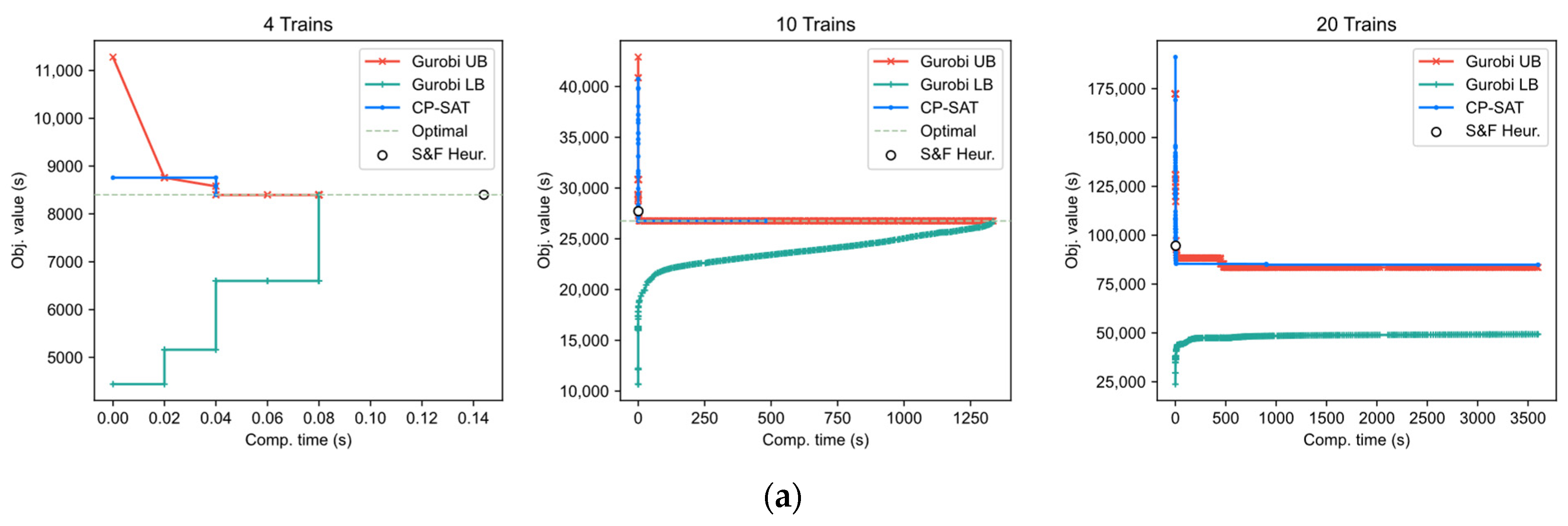
4.1.1. Computational Performance Comparison

We first conduct a series of numerical experiments concerning the solution quality and efficiency of the model applied. Specifically, we compare the computational performance (i.e., solution times, objective values, and convergence procedure) of the Gurobi solver, CP-SAT solver, and the schedule-and-fix applying the Gurobi solver (namely Gurobi-fixing) with regard to different numbers of scheduled trains.
(1)
Solution quality analysis
A series of train combination instances of the model with different numbers of trains (from 2 to 20, the combination of trains can be referred to in Appendix A) for station design Scheme-1 and -2 are generated artificially to test the solution time and objective value using different solution methods. The computational time of the instances is reported in Table 6. In Table 6, the computational time is recorded in the solution program, including the data loading, model generation, model solution, and data output. The objective value is the true objective value derived from the solver. The MIP gap reported is defined as (Upper bound–Lower bound)/Lower bound.
From Table 6, we can conclude that the model is of computational difficulties as both the commercial solver Gurobi and the open-source solver CP-SAT cannot obtain optimal solutions within 3600 s even if the number of trains is less than 20. For the Gurobi solver, the MIP gaps of the instances of 20 trains are greater than 40% for both Scheme-1 and Scheme-2. On the contrary, the schedule-and-fix heuristic approach proposed in this paper is shown to be very outstanding in terms of computational efficiency compared to the solvers. It takes less than 4 s to obtain feasible solutions for the 20-trains cases. For the small instances (the number of the train is less than or equal to 6), the objective values remain the same as the Gurobi and CP-SAT solvers, which means the optimal solution is obtained by applying the schedule-and-fix approach. However, with the amount of train growth, the objective values are worse than the ones obtained from solvers, as the heuristic nature of the schedule-and-fix approach might be stuck in the local optima in each single-train scheduling iteration. Despite this, the superior computational efficiency of the schedule-and-fix heuristic helps to accelerate the practical-scale experiments. In the following experiments, unless otherwise stated, the reported solution results are derived from the algorithm applying the schedule-and-fix heuristic approach.
From the comparison between Scheme-1 and Scheme-2, the computational times and MIP gaps of Scheme-1 usually perform better than the ones of Scheme-2, as Scheme-1 is without a flyover, and the number of candidate routes is less than Scheme-2. This phenomenon shows that the computational efficiency and quality are influenced by the number of trains and the complexity of the station layout.
(2)
Convergence procedures of the applied methods
The convergence of the instances with 4, 10, and 20 trains from Gurobi, CP-SAT, and schedule-and-fix heuristics are displayed in Figure 6. Among them, the red and green curve shows the upper and lower bound obtained from Gurobi, respectively, while the blue curve shows the current best feasible solution obtained from CP-SAT. The final solutions obtained from the schedule-and-fix heuristic (“S&F Heur.” for short) are displayed using a black dot.
From the convergence process, we can investigate the solution procedure using different methods in-depth. The corresponding instances of Scheme-1 and Scheme-2 generally show similar convergence trends. The optimal solutions are reported for 4-train and 10-train cases, as the Gurobi and CP-SAT can obtain optimal solutions within 3600 s. Gurobi and CP-SAT obtain good quality feasible solutions in very few seconds, while most of the time, the solvers update the lower bound to prove the optimality of the solutions. For the large-scale instances (40-train instances), the lower bounds are difficult to improve using the Gurobi solver.

4.1.2. Sensitivity of Parameters on Computation

(1)
Different objective functions
There are two objective functions for compressing the timetable: only minimizing the movement ending time and simultaneously minimizing the movement starting and ending time. We compare these two objective functions in terms of computational time and solution quality. The computational times, objective values, occupation rate, and the maximum number of trains of the solutions are reported in Table 7.
In Table 7, “Min d” denotes the objective function of Formulation (3), while “Min d + a” denotes the following objective function. The computational time is recorded in the solution program, and the objective value is derived from the solver. The occupation rate and capacity are calculated based on the values of the decision variables.
min f F   m M f   d m + a m
From Table 7, the study found that, in general, there is no essential difference in the quality of the solutions obtained by the two objective functions. The difference of occupation rates of corresponding instances is less than 1% except for instance S2–26. We consider the solution error due to the non-optimality results in this difference. Therefore, we apply the objective function of minimizing the total ending time of the movements in the following experiments.
(2)
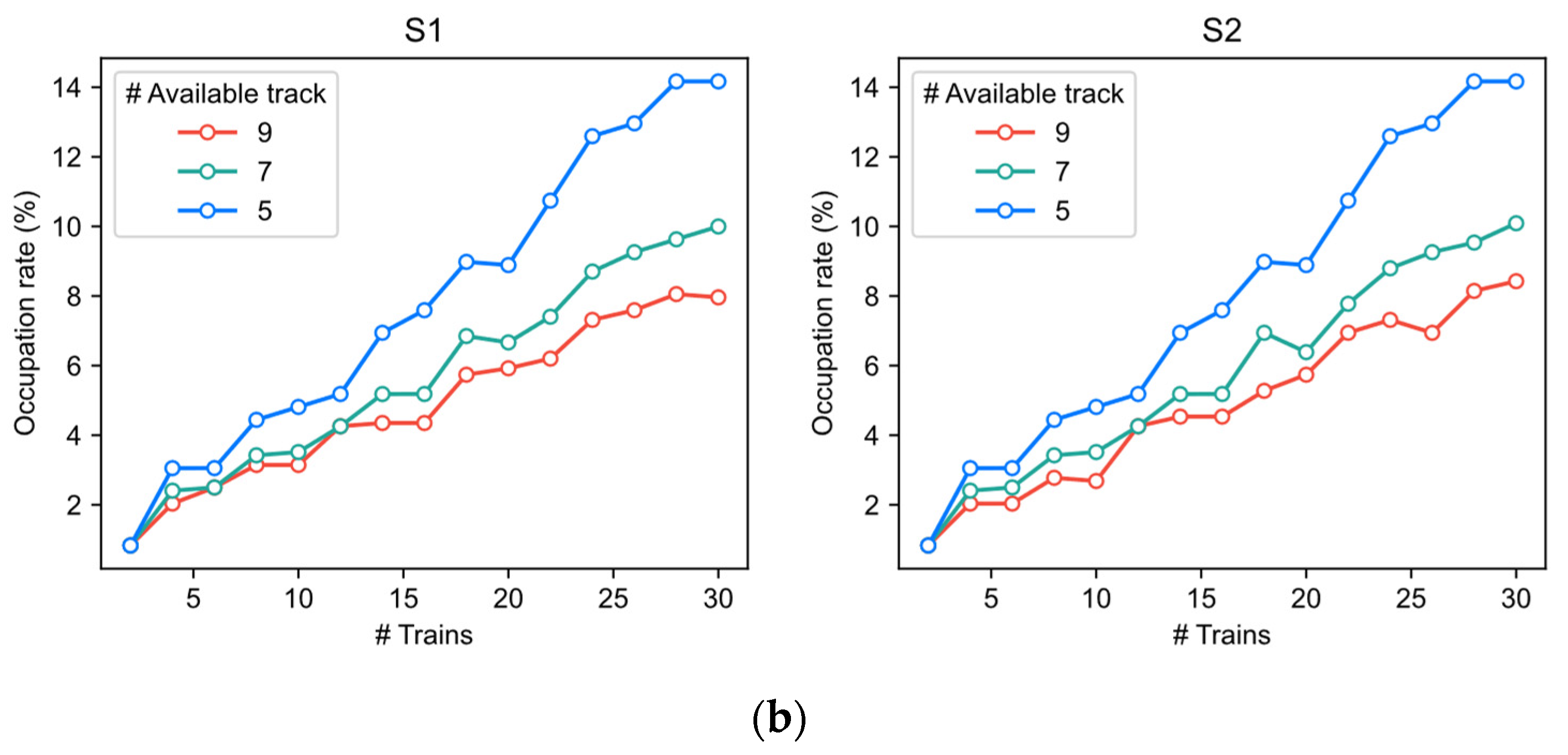
Number of available siding tracks
One major impact factor of station layout on station capacity is the number of available siding tracks, as the siding tracks provide room for train operation (i.e., passenger boarding and alighting, train turn-around, and making necessary technical inspections before going back to or after exiting from the depot). To evaluate the impact of the number of siding tracks on station capacity, we conduct three station layout variants with 9, 7, and 5 available siding tracks, and calculate the corresponding occupation rate with a different number of trains. The computational times and the occupation rates are reported in Figure 7.
Figure 7a shows that the computational time increases exponentially with the number of trains growing. With more siding tracks, the solution space of the instance would be larger, resulting in longer computational time even though the schedule-and-fix heuristic is applied. Specifically, the instance of Scheme-2 usually takes longer computational time than the corresponding instance (with the same trains and available siding tracks) of Scheme-1, as in Scheme-2, the trains departing from track 7G and 9G can choose to leave the station via the flyover or not. This flexibility of route choice enlarges the solution space, thus increasing the solution difficulties.
Concerning the occupation rate, it increases with the number of trains in general. However, the curves show a zig-zag pattern instead of a smooth linear one, as not only the number but the combination of trains influence the occupation rate. Moreover, for the instances that the number of trains is over 15, when the number of available tracks decreases from 9 to 7, the drop in the occupation rate is greater than the one when the number of available track decrease from 7 to 5. One reason for this phenomenon is that fewer available tracks might result in a severe capacity shortage, especially when more trains are scheduled.
(3)
The occupancy rate with the train number growth and the bottleneck
We analyze the growth in occupation rates of different station areas by train numbers. The growing trends of the occupation rates with the growth in train numbers are shown in Figure 8.
In Figure 8, when the train number is less than 10, the differences of occupation rate in the throat and siding track area are not noticeable, which proves that the station layout is designed reasonably in terms of capacity utilization to some extent. When the train number is greater than 20, the siding track area has a higher occupation rate than the throat areas, implying that the siding tracks are likely to be the bottleneck of the station capacity. For the throat areas, the occupation rate of the left throat is slightly higher than that of the right throat, as the left throat has a more complex structure for train arrival, departure, exiting from, and entering to depot. Therefore, the left throat might have more potential conflicts, especially when the number of turn-around trains and exiting/entering depot trains grows.

4.2. The Real-Life Case Study Analysis

In this section, we apply real-life instances with 198 trains operated in the station with the schedule-and-fix heuristic. The train combination is determined according to the operation plan design document. The capacity estimation result reported in this section can be regarded as a reference for flyover building decisions from the perspective of train operations.

4.2.1. Overall Solutions

(1)
Capacity estimation result
In this experiment, we compare two working mechanisms of the signal system, namely route-lock-route-release (RLRR for short) and route-lock-section-release (RLSR for short). Intuitively, the RLSR has less occupation time and thus can achieve higher station capacity. With a given station layout and certain train combinations, we quantitatively estimate the capacity increment of such signal system upgrades.
From Table 8, we can observe that RLSR can gain 8.25% and 8.62% capacity enhancement for Scheme-1 and Scheme-2, respectively. The compressed timetables of Scheme-1 and Scheme-2 following the RLSR mechanism are displayed in Figure 9. The horizontal axis of the figures is the time horizon, while the vertical axis represents the cells of the station. Each colored rectangle indicates a train movement occupying the associated cell in a certain period. Remarkably, the blue, yellow, and green rectangles represent arrival, dwelling, and departure movement, respectively. The train names of the movements are displayed on the corresponding dwelling rectangles.
For Scheme-1, the cell 1DG, 3DG, 7DG, 13DG, 15DG, and 17DG serve both arrival and departure movement, while other cells in the throat areas only serve a single type of movement. Without the flyover, the turn-around trains granted “BDtr” can use siding tracks 9G, 7G, 5G, and 3G for stopping. However, the departure routes of these tracks toward the BD direction occupy 7DG, which might conflict with the arrival movement from the BD direction. For Scheme-2, with the flyover, the turn-around train granted “BDtr” can use siding tracks 9G and 7G. Therefore, the departure movements of these trains only occupy 1DG and are free from conflict with the arrival trains. This spatial conflict resolution measure reduces the signal’s waiting time, increasing the station capacity.
(2)
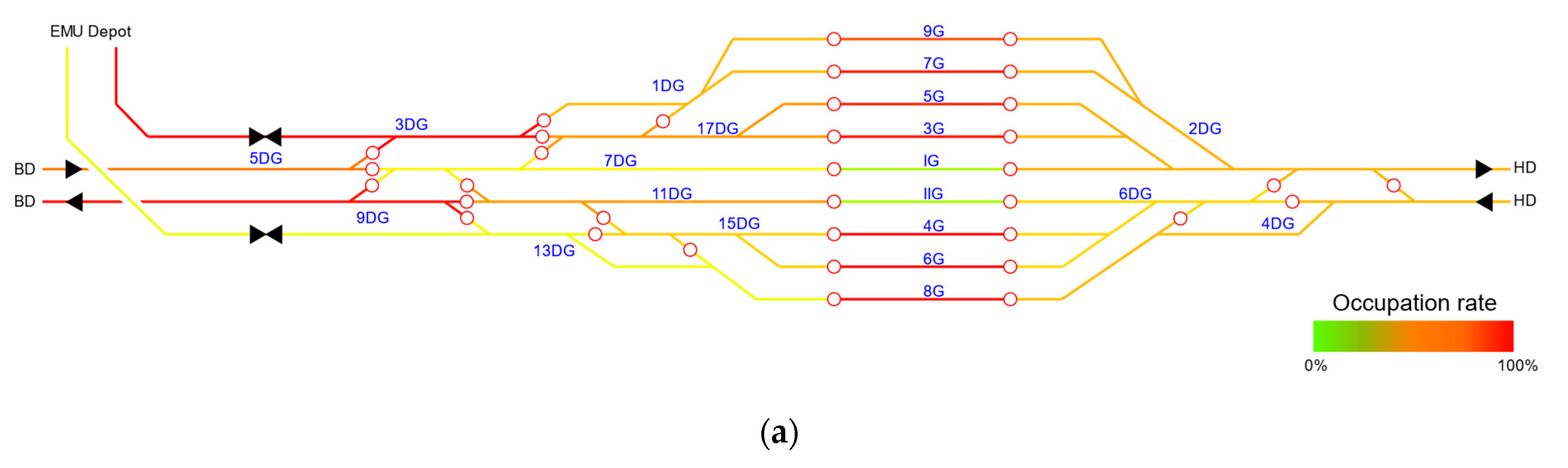
Occupation rates of track circuits
In order to display the difference of the occupation rate, we generate heat graphs displaying the occupation rate using the colors spectrum on the station layout, shown in Figure 10.
The bar charts comparing the occupation rate of different areas are displayed in Figure 11, Figure 12 and Figure 13.
From Figure 11, we can figure out that the occupation rate of the siding track area is higher than any throat area, reaching about 30%. Concerning the throat areas, the left throat has a higher occupation rate than the right throat. This characteristic of the occupation rate is identical to the small-scale instances displayed in Figure 8. Among the two station layout schemes, Scheme-2 has a lower occupation rate on the left throat, as the flyover resolves the conflicts between the arrival and departure trains. The turn-around trains granted “BDtr” stopping at siding tracks 7G and 9G only occupy one cell (1DG) instead of occupying 1DG, 17DG, 7DG, and 9DG for their departures. Specifically, we compare the occupation rate of each cell, and the results are displayed in Figure 12 and Figure 13.
For the throat areas, the occupation rates of the cells located at the right throat are identical between Scheme-1 and Scheme-2, as the flyover does not affect the movements on the right throat. However, by building the flyover, the occupation rates of the cells on the left throat varied between Scheme-1 and Scheme-2. Specifically, the occupation rate of cells 7DG and 9DG decrease dramatically by building the flyover, as the turn-around trains granted “BDtr” can depart through 1DG, instead of using 7DG and 9DG. Furthermore, the occupation rate of cell 17DG decreases slightly. On the contrary, the occupation rate of 1DG increases slightly due to the increased number of turn-around and departure trains running through the flyover.
Only the occupation rate of 7DG and 9DG for the siding tracks increases as the train running through the flyover has to stop at these two siding tracks. Benefiting from the flyover, the possibility of conflicts between arrival and departure trains on the left throat decreases so as to reduce the extra waiting time of the trains on the siding tracks. Therefore, the occupation rates of other siding tracks generally decrease.

4.2.2. Comparison of Parameter Sensitivity

(1)
Proportion of turn-around trains
The capacity performance of building such a flyover depends on the train combination. Therefore, we generate several instances with different train combinations. The instances both have 198 trains in the train set. However, the train running direction and operations are different. Detailed information on the train combinations can be referred to in Appendix A. The capacity of the proportion of variant instances is reported in Figure 14.
Figure 14 shows that Scheme-2 consistently outperforms Scheme-1 regarding the station capacity for any proportion of turn-around trains. In particular, when the proportion of turn-around trains is less than 70%, the absolute capacity value difference between Scheme-1 and Scheme-2 remains at the same level (between 10 and 30 trains, except for the case with 10% turn-around trains). However, when the proportion of turn-around trains is greater than 70%, Scheme-2 significantly benefits the capacity aspect. With the higher proportion of turn-around trains, the flyover significantly contributes to the station capacity improvement. The proportion of turn-around trains has consequences for the probability conflict between arrival and departure movements. Therefore, the effectiveness of building a flyover is determined to a great extent by the combination of trains.
(2)
Minimum turn-around time and headway
The operation parameters, such as minimum turn-around time and minimum headways, might impact the station capacity. We conduct a parameter sensitivity analysis for the two parameters mentioned above to investigate if it is possible to increase the station capacity by shortening these parameters. The relationship between station capacity and the various values of the parameters are displayed in Figure 15.
Figure 15a shows a linear trend between the minimum headway and station capacity, implying that minimum headway has a very obvious and direct effect on the station capacity. In other words, enhancing the station capacity by shortening the minimum headway is very useful. On the contrary, the minimum turn-around time performs a complex influence on station capacity, as shown in Figure 15b. Generally, there is a weak correlation between the minimum turn-around time and station capacity with the same layout scheme, i.e., the longer the minimum turn-around time, the smaller the capacity. This phenomenon can be further used to guide the capacity enhancement measurement; that is, increasing the capacity by compressing the turn-around time is very limited in general. When the turn-around time is shorter than 600 s, the difference between Scheme-1 and Scheme-2 becomes more significant, as the arrival and departure conflicts happen more frequently when the dwell times on the siding tracks are shorter.

5. Conclusions

This paper addresses a railway station capacity estimation problem for estimating the operation performance of the various design schemes. In particular, we first build a topology model to describe the layout and signal equipment of the railway station. The train operations within railway stations are described as “movement” with regard to facility occupation rules. Based on the train layout and train movement description, a mixed-integer programming model for train timetable compression is proposed to calculate the occupation rate of specific timetables, thus estimating the railway capacity of the specific layout design schemes. The schedule-and-fix heuristic algorithm is applied to solve the MIP model effectively. This method can be used to estimate the capacity utilization for stations with various layouts (i.e., different numbers of siding tracks, different connections between the siding tracks and the open track segments, and different operation parameters such as minimum headways and turn-around time limit).
Concerning the methodology used, the practical instance of the railway station capacity estimation problem is a large-scale combinatorial problem, as the existing MIP solvers find it difficult to obtain optimal solutions even if the number of trains is very low. The schedule-and-fix heuristic can accelerate the solution procedure sharply. Concerning the necessity of building a flyover to resolve the conflict of arrival and departure movements, the flyover provides capacity benefit to some extent for such a type of passenger railway station. However, only approximately 2% to 4% of the capacity improvement can be gained when the proportion of turn-around trains is less than 70%. Therefore, considering traffic combinations, building a flyover is beneficial only when the proportion of turn-around trains is significantly greater.
The station capacity result is significantly impacted by the arrival and departure headway. However, the impact of the turn-around time on station capacity is rather complicated. The result can provide hints for improving the station capacity while the infrastructure modification is not considered.
The proposed method can be applied in the real-life railway station design task, especially for the comparison and selection of the station layout design scheme. The solution algorithm can be embedded in a professional station computer-aided design program to calculate the capacity-related indices (i.e., the maximum number of trains, the occupation rate, and the bottleneck recognition result). This information can assist the engineers to better compare and trade-off the performance of the station layouts.
The limitations of this research are as follows. Cell occupation and release times are calculated by the formulations based on ideal situations, where the length and the dynamics of trains are not considered. Furthermore, the schedule-and-fix approach is not flexible enough during iteration procedures, limiting the solutions’ quality. Future research can focus on these limitations.

Author Contributions

Conceptualization, Z.L. and C.M.; methodology, Z.L.; formal analysis, C.M.; writing—original draft preparation, Z.L. and C.M.; writing—review and editing, Z.L. All authors have read and agreed to the published version of the manuscript.

Funding

This research was funded by the Science and Technology Research and Development Project of China State Railway Group Company, Ltd. (Grant No. N2022X018).

Data Availability Statement

The data applied in the research is unavailable due to privacy.

Acknowledgments

The author sincerely thanks the technical support from Lingyun Meng, Jianrui Miao, and Xiaojie Luan for their technical support.

Conflicts of Interest

The authors declare no conflict of interest.

Appendix A

Table A1. The combination of trains.
Turn-Around Train ProportionEntering/Exiting the DepotTurn-AroundPassing ThroughTotal
BDHDBDHDWith StopWithout Stop
0.038220010632198
0.138221648632198
0.2382226146632198
0.3382236244632198
0.4382246342632198
0.538225644632198
0.638226654018198
0.73620776500198
0.82610877500198
0.9160978500198
1.0001059300198

Appendix B

Table A2. Default cell occupation time parameters.
RouteMovement TypeSequenceCellPreoccupation Time (s)Release Time (s)
SA2Arrival14DG3000
SA2Arrival26DG3000
SA2Arrival3IIG3000
SA4Arrival14DG24060
SA4Arrival26DG2400
SA4Arrival34G2400
SA6Arrival14DG24060
SA6Arrival26DG2400
SA6Arrival36G2400
SA8Arrival14DG24060
SA8Arrival28G2400
XA1Arrival15DG3000
XA1Arrival27DG3000
XA1Arrival3IG3000
XA3Arrival15DG24060
XA3Arrival23DG2400
XA3Arrival317DG2400
XA3Arrival43G2400
XA5Arrival15DG24060
XA5Arrival23DG2400
XA5Arrival317DG2400
XA5Arrival45G2400
XA7Arrival15DG24060
XA7Arrival23DG2400
XA7Arrival31DG2400
XA7Arrival47G2400
XA9Arrival15DG24060
XA9Arrival23DG2400
XA9Arrival31DG2400
XA9Arrival49G2400
EA3Arrival from depot13DG24060
EA3Arrival from depot217DG2400
EA3Arrival from depot33G2400
EA4Arrival from depot113DG24060
EA4Arrival from depot215DG2400
EA4Arrival from depot34G2400
EA5Arrival from depot13DG24060
EA5Arrival from depot217DG2400
EA5Arrival from depot35G2400
EA6Arrival from depot113DG24060
EA6Arrival from depot215DG2400
EA6Arrival from depot36G2400
EA7Arrival from depot13DG24060
EA7Arrival from depot21DG2400
EA7Arrival from depot37G2400
EA8Arrival from depot113DG24060
EA8Arrival from depot28G2400
EA9Arrival from depot13DG24060
EA9Arrival from depot21DG2400
EA9Arrival from depot39G2400
SD2Departure1IIG060
SD2Departure211DG30060
SD2Departure39DG30060
SD3Departure13G060
SD3Departure217DG60120
SD3Departure37DG60180
SD3Departure49DG60180
SD4Departure14G060
SD4Departure215DG60120
SD4Departure311DG60160
SD4Departure49DG60180
SD5Departure15G060
SD5Departure217DG60120
SD5Departure37DG60180
SD5Departure49DG60180
SD6Departure16G060
SD6Departure215DG60120
SD6Departure311DG60180
SD6Departure49DG60180
SD7Departure17G060
SD7Departure21DG60120
SD7Departure317DG60120
SD7Departure47DG60180
SD7Departure59DG60180
SD8Departure14DG060
SD8Departure28G60120
SD8Departure313DG60180
SD8Departure49DG60180
SD9Departure11DG060
SD9Departure217DG60120
SD9Departure37DG60180
SD9Departure49DG60180
SDF7Departure17G060
SDF7Departure21DG60180
SDF9Departure19G060
SDF9Departure21DG60180
XD1Departure1IG060
XD1Departure22DG30060
XD3Departure13G060
XD3Departure22DG60180
XD5Departure15G060
XD5Departure22DG60180
XD7Departure17G060
XD7Departure22DG60180
XD9Departure19G060
XD9Departure22DG60180
ED3Departure to depot13G060
ED3Departure to depot217DG60120
ED3Departure to depot33DG60180
ED4Departure to depot14G060
ED4Departure to depot215DG60120
ED4Departure to depot313DG60180
ED5Departure to depot15G060
ED5Departure to depot217DG60120
ED5Departure to depot33DG60180
ED6Departure to depot16G060
ED6Departure to depot215DG60120
ED6Departure to depot313DG60180
ED7Departure to depot17G060
ED7Departure to depot21DG60120
ED7Departure to depot33DG60180
ED8Departure to depot18G060
ED8Departure to depot213DG60180
ED9Departure to depot19G060
ED9Departure to depot21DG60120
ED9Departure to depot33DG60180

References

  1. UIC. UIC Code 406: Capacity, 1st ed.; International Union of Railways: Paris, France, 2004. [Google Scholar]
  2. Khadem-Sameni, M.; Preston, J.; Armstrong, J. Railway capacity challenge: Measuring and managing in Britain. In Proceedings of the ASME/IEEE Joint Rail Conference, Urbana, IL, USA, 27–29 April 2010; Volume 49071, pp. 571–578. [Google Scholar]
  3. Malavasi, G.; Molková, T.; Ricci, S.; Rotoli, F. A synthetic approach to the evaluation of the carrying capacity of complex railway nodes. J. Rail Transp. Plan. Manag. 2014, 4, 28–42. [Google Scholar] [CrossRef]
  4. Wang, J.; Yu, Y.; Kang, R.; Wang, J. A novel space-time-speed method for increasing the passing capacity with safety guaranteed of railway station. J. Adv. Transp. 2017, 2017, 6381718. [Google Scholar] [CrossRef]
  5. Veselý, P. Methodology for capacity calculation in railway stations used in is kango. Perners Contacts 2013, 8, 100–106. [Google Scholar]
  6. Bychkov, I.; Kazakov, A.; Lempert, A.; Zharkov, M. Modeling of railway stations based on queuing networks. Appl. Sci. 2021, 11, 2425. [Google Scholar] [CrossRef]
  7. Yuan, J.; Hansen, I.A. Optimizing capacity utilization of stations by estimating knock-on train delays. Transp. Res. Part B Methodol. 2007, 41, 202–217. [Google Scholar] [CrossRef]
  8. Corriere, F.; Di Vincenzo, D.; Guerrieri, M. A logic fuzzy model for evaluation of the railway station’s practice capacity in safety operating conditions. Arch. Civ. Eng. 2013, 3–19. [Google Scholar] [CrossRef]
  9. Han, S.; Yue, Y.; Zhou, L. Carrying capacity of railway station by microscopic simulation method. In Proceedings of the 17th International IEEE Conference on Intelligent Transportation Systems (ITSC), Qingdao, China, 8–11 October 2014; IEEE: New York, NY, USA, 2014; pp. 2725–2731. [Google Scholar]
  10. Zhong, M.; Yue, Y.; Li, D. Analyzing and evaluating infrastructure capacity of railway passenger station by mesoscopic simulation method. In Proceedings of the 2018 International Conference on Intelligent Rail Transportation (ICIRT), Singapore, 12–14 December 2018; IEEE: New York, NY, USA, 2018; pp. 1–5. [Google Scholar]
  11. Bulíček, J.; Nachtigall, P.; Široký, J.; Tischer, E. Improving single-track railway line capacity using extended station switch point area. J. Rail Transp. Plan. Manag. 2022, 24, 100354. [Google Scholar] [CrossRef]
  12. Armstrong, J.; Preston, J. Capacity utilisation and performance at railway stations. J. Rail Transp. Plan. Manag. 2017, 7, 187–205. [Google Scholar] [CrossRef]
  13. Yuan, J.; Hansen, I.A. Analysis of scheduled and real capacity utilisation at a major Dutch railway station. WIT Trans. Built Environ. 2004, 74, 593–602. [Google Scholar]
  14. Landex, A. Station capacity. In Proceedings of the 4th International Seminar on Railway Operations Research, Rome, Italy, 16–18 February 2011. [Google Scholar]
  15. Johansson, I.; Weik, N. Strategic assessment of railway station capacity–Further development of a UIC 406-based approach considering timetable uncertainty. In Proceedings of the 9th International Conference on Railway Operations Modelling and Analysis (ICROMA), RailBeijing 2021, Beijing, China, 3–7 November 2021. [Google Scholar]
  16. Zhong, Q.; Yang, R.; Zhong, Q. Equivalences between analytical railway capacity methods. J. Rail Transp. Plan. Manag. 2023, 25, 100367. [Google Scholar] [CrossRef]
  17. Kavička, A.; Diviš, R.; Veselý, P. Railway station capacity assessment utilizing simulation-based techniques and the UIC406 method. In Proceedings of the 32nd European Modeling & Simulation Symposium (EMSS 2020), CAL-TEK SRL, Online, 16–18 September 2020. [Google Scholar]
  18. Lindner, T. Applicability of the analytical UIC Code 406 compression method for evaluating line and station capacity. J. Rail Transp. Plan. Manag. 2011, 1, 49–57. [Google Scholar] [CrossRef]
  19. Gašparík, J.; Zitrický, V. A new approach to estimating the occupation time of the railway infrastructure. Transport 2010, 25, 387–393. [Google Scholar] [CrossRef]
  20. UIC. UIC Code 406: Capacity, 2nd ed.; International Union of Railways: Paris, France, 2013. [Google Scholar]
  21. Sameni, M.K.; Preston, J.; Sameni, M.K. Evaluating efficiency of passenger railway stations: A DEA approach. Res. Transp. Bus. Manag. 2016, 20, 33–38. [Google Scholar]
  22. Jovanović, P.; Pavlović, N.; Belošević, I.; Milinković, S. Graph coloring-based approach for railway station design analysis and capacity determination. Eur. J. Oper. Res. 2020, 287, 348–360. [Google Scholar] [CrossRef]
  23. Ignatov, A.N.; Naumov, A.V. On the Problem of increasing the railway station capacity. Autom. Remote Control. 2021, 82, 102–114. [Google Scholar] [CrossRef]
  24. Sels, P.; Waquet, B.; Dewilde, T.; Cattrysse, D.; Vansteenwegen, P. Calculation of realistic railway station capacity by platforming feasibility checks. In Proceedings of the 2nd International Conference on Models and Technologies for Intelligent Transport Systems (MT-ITS): MTITS2011, Leuven, Belgium, 22–24 June 2011; pp. 22–24. [Google Scholar]
  25. Guo, B.; Zhou, L.; Yue, Y.; Tang, J. A study on the practical carrying capacity of large high-speed railway stations considering train set utilization. Math. Probl. Eng. 2016, 2016, 2741479. [Google Scholar] [CrossRef]
  26. Dollevoet, T.; Huisman, D.; Kroon, L.; Schmidt, M.; Schöbel, A. Delay management including capacities of stations. Transp. Sci. 2015, 49, 185–203. [Google Scholar] [CrossRef]
  27. Javadian, N.; Sayarshad, H.R.; Najafi, S. Using simulated annealing for determination of the capacity of yard stations in a railway industry. Appl. Soft Comput. 2011, 11, 1899–1907. [Google Scholar] [CrossRef]
  28. Lu, G.; Ning, J.; Liu, X.; Nie, Y.M. Train platforming and rescheduling with flexible interlocking mechanisms: An aggregate approach. Transp. Res. Part E Logist. Transp. Rev. 2022, 159, 102622. [Google Scholar] [CrossRef]
  29. Hansen, I.; Pachl, J. Railway Timetabling and Operations: Analysis, Modelling, Optimisation, Simulation, Performance, Evaluation; Eurail Press: Utrecht, The Netherlands, 2014. [Google Scholar]
  30. Liao, Z. PyStationCapacity [Source code]. Available online: https://gitee.com/lzw37/py-station-capacity (accessed on 28 August 2023).
Figure 1. The layout variants of a railway station: (a) without flyover; and (b) with a flyover.
Mathematics 11 03727 g001
Figure 2. The topological model of the station.
Mathematics 11 03727 g002
Figure 3. Train arrival, departure, and dwell movements. (a) Train routes. (b) Cell occupation.
Mathematics 11 03727 g003
Figure 4. Layout design schemes of BDD Station. (a) Scheme-1 (without flyover). (b) Scheme-2 (with flyover).
Mathematics 11 03727 g004aMathematics 11 03727 g004b
Figure 5. Heterogeneous train composition for the case study.
Mathematics 11 03727 g005
Figure 6. Convergence procedure of the objective value by different solution methods. (a) Scheme-1 (without flyover). (b) Scheme-2 (with flyover).
Mathematics 11 03727 g006aMathematics 11 03727 g006b
Figure 7. The impact of the number of available siding tracks on computational performance. (a) Computational time. (b) Overall occupation rate.
Mathematics 11 03727 g007aMathematics 11 03727 g007b
Figure 8. The relations between the occupation rate of track circuits and train numbers by schemes.
Mathematics 11 03727 g008
Figure 9. The compressed timetables of different layout schemes. (a) Scheme-1 (without flyover). (b) Scheme-2 (with flyover).
Mathematics 11 03727 g009
Figure 10. The occupation rate of the track circuit by different layout schemes. (a) Without flyover. (b) With flyover.
Mathematics 11 03727 g010aMathematics 11 03727 g010b
Figure 11. Track circuit occupation comparison between train dwelling tracks and throat areas.
Mathematics 11 03727 g011
Figure 12. Track circuit occupation rate of left and right-hand-side throat areas. (a) Left throat. (b) Right throat.
Mathematics 11 03727 g012
Figure 13. Track circuit occupation comparison between north bound and south bound siding track areas. (a) Left to right tracks. (b) Right to left tracks.
Mathematics 11 03727 g013
Figure 14. Capacity variation by proportion of turn-around trains.
Mathematics 11 03727 g014
Figure 15. Capacity variation by minimum turn-around time. (a) Minimum headway rate. (b) Minimum turn-around time.
Mathematics 11 03727 g015
Table 1. Comparison of the solution methods of railway capacity estimation.
PublicationProblemModel CategorySolution Method
Malavasi et al. [3]Station capacityAnalyticalCalculation formulation and parameter calibration
Wang et al. [4]Line capacityAnalyticalCalculation formulation and parameter calibration
Veselý [5]Station capacityAnalyticalCalculation formulation and parameter calibration
Bychkov et al. [6]Station capacityAnalyticalQueuing network
Yuan and Hansen [7]Knock-on delay estimationAnalyticalStochastic model
Corriere et al. [8]Station capacityAnalyticalLogic fuzzy model
Han et al. [9]Station capacityAnalytical + SimulationMicroscopic simulation
Zhong et al. [10]Station capacitySimulationMesoscopic simulation
Bulíček et al. [11]Station structure improvementSimulationMesoscopic simulation
Armstrong and Preston [12]Station capacityData-drivenStatistical
Yuan and Hansen [13]Station capacityData-drivenStatistical
Landex [14]Station capacityUIC 406Timetable compression via simulation
Johansson and Weik [15]Station capacityUIC 406Timetable compression via optimization
Zhong et al. [16]Station capacityUIC 406ComRec + triangular-gap-problem + max-plus algebra
Kavička et al. [17]Station capacityUIC 406MesoRail
Gašparík [19]Station capacityUIC 406Conceptual framework
Sameni et al. [21]Technical efficiency and service effectiveness estimationOptimizationData envelopment analysis
Jovanović et al. [22]Station capacityOptimizationTwo-stage optimization method
Naumov [23]Station capacity improvementOptimizationMIP model
Sels et al. [24]Station capacityOptimizationMIP for track allocation
Guo et al. [25]Station capacityOptimizationMIP
Dollevoet et al. [26]Station capacityOptimizationTrain delay management model
Javadian et al. [27]Station capacityOptimizationSimulated annealing
Table 2. Notations.
Table 2. Notations.
NotationsDescriptions
Elements and sets
Q A constant number that is big enough
F Train set
f Train element
M f Movement set of train f at the station
m Movement element
R m The possible route of movement m
r Route element
C r The occupied cell set when the train is using route r
C m The possible cell set occupied by movement m
c Cell element
Parameters (numbers)
δ m m i n , δ m m a x The minimum and maximum duration of movement m
l m d e p , h m d e p Earliest and latest ending time of movement m
l m a r r , h m a r r Earliest and latest beginning time of movement m
θ r , c The preoccupation time of cell c when the movement is using route r
β r , c The additional release time of cell c when the movement is using route r
η r 1 , r 2 A binary parameter, 1 indicates route r 1 has a physical connection with route r 2 , 0 otherwise
Projection
g m A projection from one movement to the other. m = g ( m ) indicates that, for the same train, the movement m happens immediately following movement m . If the movement m is the last movement of the train, g m = m n u l l
Table 3. Variables.
Table 3. Variables.
VariablesDescriptions
a m The beginning time of movement m
d m The ending time of movement m
x m , r Binary variable, 1 indicates movement m applies route r to operate, 0 otherwise.
y c , m 1 , m 2 Binary variable, 1 indicates that movement m 1 occupies cell c earlier than movement m 2 , 0 otherwise.
s m , c The starting time of movement m occupying cell c
e m , c The ending time of movement m occupying cell c
Table 4. Default track circuit occupation time parameters (in seconds).
Train MovementMin Preoccupation TimeMin Release Time
StopNon-StopStopNon-Stop
Arrival24030000
Departure6030018060
Table 5. Required dwell time parameters (in seconds).
Train TypeMinimum Dwell TimeMaximum Dwell Time
Before entering depot9001800
After exiting from depot9001800
Turn-around7201200
Passing through with stop120900
Table 6. The computational times and objective values.
Instance# TrainsGurobiCP-SATGurobi Fixing
Comp. Time (s)Obj Value (Min)Gap (%)Comp. Time (s)Obj Value (Min)Gap (%)Comp. Time (s)Obj Value (Min)
Scheme-12<0.119200.00%0.119200.00%0.01920
40.184000.00%0.184000.00%0.18400
61.511,9400.00%0.511,9400.00%0.311,940
872.219,3200.00%4.219,3200.00%0.520,820
101336.026,7600.00%484.726,7600.00%0.727,720
123600.837,92031.46%3623.737,92036.03%1.040,980
143605.147,58026.26%3606.747,16035.84%1.351,480
163604.757,78035.97%3609.658,62043.01%1.861,500
183604.874,94043.58%3627.171,34046.04%2.579,440
203601.983,52040.96%3690.584,90048.59%2.994,620
Scheme-22<0.119200.00%<0.119200.00%0.01920
40.584000.00%0.184000.00%0.18400
64.011,9400.00%0.711,9400.00%0.311,940
864.619,3200.00%4.219,3200.00%0.520,700
102387.526,7600.00%253.326,7600.00%0.628,080
123601.237,56030.14%3606.437,44039.55%1.138,160
143604.946,68029.26%3604.447,22037.23%1.455,020
163604.557,48037.72%3610.957,24042.88%1.961,500
183604.772,54043.89%3610.070,98048.73%2.677,400
203604.084,96043.17%3607.982,20050.46%3.193,000
Table 7. Solution comparison using different objective functions.
Instances (Scheme-#Trains)Comp. Time (s)Obj. Value (s)Occupation Rate (%)Capacity
(Max #Trains)
Min dMin d+aMin dMin d + aMin dMin d + aMin dMin d + a
S1-20.00.0192036000.83%0.83%240240
S1-40.10.1840014,9402.04%2.04%196196
S1-60.30.311,94021,9602.50%2.50%240240
S1-80.50.520,82037,8003.15%3.15%254254
S1-100.70.627,72051,3003.15%3.52%318284
S1-121.01.040,98077,7604.26%4.26%282282
S1-141.31.351,48095,5804.35%4.35%322322
S1-161.81.961,500115,3804.35%4.35%368368
S1-182.42.579,440149,4005.74%5.28%314341
S1-202.92.994,620178,7405.92%5.93%338338
S1-223.83.8114,120226,2606.20%6.57%355335
S1-244.84.7136,320276,4807.31%7.31%328328
S1-266.05.7164,400309,6007.59%7.59%342342
S1-287.26.8190,260348,4808.06%8.61%348325
S1-307.47.4195,480399,2407.96%8.42%377356
S2-20.10.0192036000.83%0.83%240240
S2-40.10.1840014,9402.04%2.04%197197
S2-60.30.311,94021,9602.04%2.04%295295
S2-80.50.520,70037,6202.78%2.78%288288
S2-100.60.728,08052,2002.69%2.69%372372
S2-121.01.138,16077,2204.26%4.26%282282
S2-141.41.455,020102,2404.54%4.54%309309
S2-161.91.961,500116,8204.54%4.63%353346
S2-182.52.677,400146,1605.28%5.00%341360
S2-202.92.993,000178,5605.74%5.74%348348
S2-224.03.8116,520217,4406.94%6.48%317339
S2-245.14.8138,780261,5407.31%7.31%328328
S2-266.25.9146,760301,3206.94%7.96%374327
S2-287.47.0174,060344,7008.15%8.43%344332
S2-308.17.7195,900380,7008.43%8.43%356356
Table 8. Comparison between RLRR and RLSR working mechanisms.
SchemeRoute-Lock-Route-Release (RLRR)Route-Lock-Section-Release (RLSR)Capacity Improvement by Applying RLSR
Occupation RateObj. ValueCapacityOccupation RateObj. ValueCapacity
S148.61%8,870,76040744.91%8,448,7804418.25%
S246.67%8,636,40042442.96%7,597,2604618.62%
Disclaimer/Publisher’s Note: The statements, opinions and data contained in all publications are solely those of the individual author(s) and contributor(s) and not of MDPI and/or the editor(s). MDPI and/or the editor(s) disclaim responsibility for any injury to people or property resulting from any ideas, methods, instructions or products referred to in the content.

