CAM-FRN: Class Attention Map-Based Flare Removal Network in Frontal-Viewing Camera Images of Vehicles

Abstract

In recent years, active research has been conducted on computer vision and artificial intelligence (AI) for autonomous driving to increase the understanding of the importance of object detection technology using a frontal-viewing camera. However, using an RGB camera as a frontal-viewing camera can generate lens flare artifacts due to strong light sources, components of the camera lens, and foreign substances, which damage the images, making the shape of objects in the images unrecognizable. Furthermore, the object detection performance is significantly reduced owing to a lens flare during semantic segmentation performed for autonomous driving. Flare artifacts pose challenges in their removal, as they are caused by various scattering and reflection effects. The state-of-the-art methods using general scene image retain artifactual noises and fail to eliminate flare entirely when there exist severe levels of flare in the input image. In addition, no study has been conducted to solve these problems in the field of semantic segmentation for autonomous driving. Therefore, this study proposed a novel lens flare removal technique based on a class attention map-based flare removal network (CAM-FRN) and a semantic segmentation method using the images in which the lens flare is removed. CAM-FRN is a generative-based flare removal network that estimates flare regions, generates highlighted images as input, and incorporates the estimated regions into the loss function for successful artifact reconstruction and comprehensive flare removal. We synthesized a lens flare using the Cambridge-driving Labeled Video Database (CamVid) and Karlsruhe Institute of Technology and Toyota Technological Institute at Chicago (KITTI) datasets, which are road scene open datasets. The experimental results showed that semantic segmentation accuracy in images with lens flare was removed based on CAM-FRN, exhibiting 71.26% and 60.27% mean intersection over union (mIoU) in the CamVid and KITTI databases, respectively. This indicates that the proposed method is significantly better than state-of-the-art methods.

1. Introduction

There is an increasing need for object detection and recognition technologies to prevent accidents during autonomous driving by precisely identifying the road conditions around a vehicle. In recent years, semantic segmentation methods have been used to identify objects on roads accurately, and further studies are being conducted to enhance segmentation performance [1,2,3,4,5,6,7]. However, there are limitations when detecting objects using a frontal-viewing camera. Ceccarelli et al. [8] reported that a flare is one of the causes of the failure of an RGB camera in autonomous driving vehicle applications.

Figure 1 shows the generation process of a lens flare. To acquire a normal image, the light source and object must reach the image sensor through a correct path, as indicated by the figure’s dotted gray and black solid lines. However, unintentional reflection and scattering (indicated by orange and yellow solid lines in Figure 1) may occur by a light ray from a light source and damage or foreign substance in the front part of a lens. As shown in Figure 1, an artifact owing to a light source is overlaid on top of the existing scene as a layer, which generates a lens flare [9,10]. This significantly degrades semantic segmentation performance and can lead to inaccurate decisions in dangerous situations during autonomous driving.

Figure 2 shows the effects of a lens flare on semantic segmentation, which is required for object detection during autonomous driving. Figure 2d shows an image damaged by a lens flare. When semantic segmentation by DeepLabV3+ [7] is performed using the image in Figure 2d, the error in the segmentation result worsens to the extent that objects are undetectable, as shown in Figure 2e. On comparing Figure 2c,e, which show the semantic segmentation results by DeepLabV3+ [7] of the original image, it was found that a lens flare is an obstacle in autonomous driving as it negatively affects the object detection system for autonomous driving.

A lens flare can be prevented to a certain extent by improving the camera hardware. An anti-reflective coating can be applied to a lens, or a lens flare can be suppressed by improving the camera barrel or lens hood. However, such hardware improvement measures are expensive and can prevent only certain types of lens flares [11,12,13]. Another method involves software improvement. In particular, there are handcrafted feature-based methods for automatically detecting and removing flares in images with a lens flare [10,14,15,16,17,18]. Because the types of flares that can be removed using handcrafted feature-based methods are limited, such methods are difficult to apply to autonomously driving vehicles. Therefore, we performed semantic segmentation tasks after removing the lens flare using deep learning methods.

However, there is a limitation to removing a lens flare using deep learning methods. There is insufficient training data for supervised learning, and extensive amounts of time and effort are required to obtain a pair of images with and without a lens flare at the same location and time. When these image pairs are being acquired, the data acquisition process becomes complicated owing to certain conditions (e.g., the angle at which the light is radiated onto the camera lens front, location of the light source, etc.) that must be satisfied to generate a lens flare. Even when a pair of images with and without a lens flare is obtained from the same scene, the two images cannot be guaranteed to be captured under the same conditions. Therefore, we used a lens flare generation method proposed by Wu et al. [9] to solve the issue of insufficient training data by classifying lens flares into scattering and reflective cases. To obtain a scattering flare, scattering lens flare images were generated using the physics-based data generation method based on the physics of a lens flare. Conversely, a reflective flare was obtained directly through experiments because obtaining such type of data through a simulation is rather difficult. Therefore, they created a dataset for a single image flare removal (SIFR) task by synthesizing a lens flare with clean images without a flare. Data synthesis is conducted to create a lens flare removal dataset to be used for training, considering a lens flare, as shown in Figure 1, is overlaid on top of an existing scene. Accordingly, previous work [9] proposed synthesizing lens flare artifacts with images without a flare to generate the training data. Therefore, in this study, we used the method proposed in [9] to synthesize lens flare artifacts with CamVid [19] and KITTI [20] dataset inputs wherein a semantic segmentation label exists.

In addition, flare artifacts can be a combination of different types of scattering and reflection artifacts. Considering the various artifacts when removing flare remains a challenge, and in some cases the network cannot remove them successfully, leaving an artifactual noises [9,21,22]. Furthermore, in some cases the network cannot remove the flare if there exist the severe level of flare in the input image [23]. To address these issues, we propose a generative-based flare removal network that estimates the flare region in an image, and generates additional images that highlight it in addition to serving as input to the network. In addition, we incorporate the estimated flare region into a loss function to successfully reconstruct objects occluded by the artifact and effectively remove flare artifacts that appear throughout the image.

This study proposes a novel lens flare removal technique based on a class attention map-based flare removal network (CAM-FRN) and a semantic segmentation method using images with the lens flare removed. The novelty of the proposed method with respect to previous studies is as follows.

• This study is the first to solve the lens flare problem in the field of semantic segmentation for frontal-viewing camera images using CAM-FRN as a solution;
• We propose a class attention map (CAM) module utilizing a ResNet-50 classifier to detect and remove areas damaged by lens flare artifacts effectively. Additionally, we incorporate the obtained flare regions into the network’s objective function, enabling efficient lens flare removal;
• We propose an atrous convolution dual channel attention residual block (ADCARB) that estimates the features corrupted by flare via channel attention and sigmoid function while performing multi-scale learning utilizing dilated convolution [24] to remove flare.
• By applying self-attention to the latent space, global information is considered. To consider local information simultaneously, the latent space before and after self-attention is fused and then delivered to the decoder. Lastly, the CAM-FRN model with code and the flare-generated image database are publicly disclosed for a fair performance evaluation by other researchers via Github site [25].

The remainder of this paper is organized as follows: Section 2 introduces previous research methods related to this study. Section 3 explains the details of the proposed method. Section 4 analyzes the experimental results, and Section 5 presents the discussion. Lastly, Section 6 concludes the study and presents future research directions.

2. Related Works

Research on lens flare removal can be categorized into two main areas: general scene image environment, focusing on image quality improvement, and vehicle frontal viewing camera image environment, emphasizing semantic segmentation accuracy. Notably, the latter domain lacks prior research dedicated to solving the lens flare problem. In contrast, the former domain has existing studies proposing lens flare removal methods; however, these methods predominantly concentrate on enhancing image quality and do not address the specific objective of improving semantic segmentation accuracy.

2.1. Studies on Image Quality Improvement in General Scene Images

Previous studies that have proposed lens flare removal in general scene images can be categorized into hardware- and software-based methods.

2.1.1. Hardware-Based Methods

Several studies have attempted different methods to mitigate a lens flare through camera hardware and optical design. First, an anti-reflective coating is applied to the camera lens to prevent flare artifacts from being generated. However, considering an anti-reflective coating is only effective for suppressing and removing a lens flare when a light ray comes in at a specific angle under the appropriate conditions, it cannot be used as a solution for all lens flare artifacts. Boynton et al. [11] proposed a simulated-eye design (SED) wherein the camera interior is filled with liquid, which prevents unintentional reflection in a lens by acting as an anti-reflective coating. However, this method requires a complicated camera design compared with a general RGB camera, which increases the costs. Unlike previous methods that involved analyzing a lens flare in a two-dimensional image, Raskar et al. [12] demonstrated that lens flares occur in a four-dimensional light ray space and statistically analyzed flare artifacts generated inside a camera. However, as mentioned in [12], their proposed method cannot eliminate the streaks of light appearing on the aperture and the diffraction effect and cannot resolve the issue of light glare caused by the surrounding environment, such as fog. Additionally, the blooming phenomenon caused by a sensor and the purple-fringing phenomenon cannot be resolved, considering a lens flare cannot be removed if a light source is expanded, as in the case of vehicle headlights. Talvala et al. [13] proposed a method for analyzing and removing veiling glare and lens flare artifacts for diverse kinds of digital cameras by configuring an occlusion mask based on the measured data and selectively blocking light that triggers flare and glare.

2.1.2. Software-Based Methods

The hardware-based lens flare removal methods explained above are generally applied to acquire camera images by analyzing certain types of flare and hence, cannot prevent or remove various types of artifacts. Moreover, additional costs are required considering cameras require additional design modifications. To overcome these drawbacks, software-based methods for detecting and removing a flare in images have been developed based on image processing algorithms, which can be roughly classified into handcrafted feature-based and deep feature-based methods.

(1)

Handcrafted Feature-Based Methods

Wu et al. [14] proposed a method to extract shadows in an image through Bayesian optimization. This method, however, requires a user to provide information about the shadows. Asha et al. [15] proposed a method for removing bright spots generated when a scene having a strong light source is captured by a camera. However, the proposed method could only be applied to certain types of artifacts or bright spots. Chabert et al. [16] proposed a two-step post-processing method for detecting the region damaged by a lens flare in an image and restoring the damaged region. However, the method proposed in [16] is also effective in removing certain flare types, such as ghosting; however, it is ineffective for other types of flare. Similar to [15,16], Vitoria et al. [17] proposed a method for automatically detecting the flare region and estimating and restoring a mask for the detected region. However, their method only detects and removes flare spots and ghosting artifacts caused by the reflection of lens components inside a camera instead of detecting and removing various types of lens flare artifacts. Koreban et al. [18] proposed a method to mitigate a flare using images of two frames captured by a moving camera. The method proposed in [18] is specialized for a specific type of flare and requires continuous images. Zhang et al. [10] removed a flare in an image by decomposing the image damaged by a flare into the scene and flare layers and eliminated the effects of a flare by adjusting the brightness and color balance of the scene layer. However, segmentation of the scene layer and lens flare layer may not work appropriately if the texture feature is not evidently exposed, and the color of a local object may be distorted.

(2)

Deep Feature-Based Methods

Deep learning technologies have been gaining wide attention in recent years and have been widely used in restoration tasks. In particular, research is actively being conducted for the cases where images are damaged owing to environmental factors such as fog or rain [21,22]. However, there is limited research on removing artifacts generated inside a camera by a strong light source. Lens flare removal tasks are difficult to solve because distinguishing a light source from a flare is difficult, and obtaining paired data on whether a flare exists is challenging. Considering the above difficulties, the following deep learning-based studies examined different methods for removing lens flare artifacts generated in the process of acquiring images.

Wu et al. [9] successfully developed lens flare removal methods based on deep learning methods by focusing on the difficulty in obtaining pairs of images with or without a lens flare to obtain only the images with flare artifacts. Moreover, they proposed a semi-synthetic data synthesis technique for creating flare-damaged images using two types of flare artifacts. And a flare removal method using U-Net [26] architecture for removing a flare in an image is used. This method is more outstanding than other handcrafted-based methods for a lens flare. However, it removes artifacts as well as the light source, and the light source is synthesized through post-processing; however, the method cannot accurately remove flares. Qiao et al. [23] proposed an unpaired dataset called the “unpaired flare removal (UFR) dataset” by focusing on the fact that it is challenging to acquire a paired dataset for flare removal tasks. Furthermore, they observed that information about a flare, such as its shape and color, is in the light source and hence, conducted unsupervised learning based on the observation result. Light source mask and flare mask were estimated within an image using the encoder–decoder structure. And the flare removal and generator modules based on a cycle-consistent generative adversarial network (CycleGAN) were trained using the two masks, flare images, and flare-free images. Although this method can generalize flare images in real life through unsupervised learning, it inadequately removes lens flare artifacts found throughout an image.

As seen above, previous studies concentrated on improving the quality of general scene images through lens removal rather than improving the semantic segmentation accuracy. Therefore, no study has examined the solution for the lens flare problem in the field of semantic segmentation in front-viewing camera images captured by a vehicle. A more detailed explanation is provided in the following subsection.

2.2. Studies on Improving the Semantic Segmentation Accuracy in Frontal-Viewing Camera Images of a Vehicle

Previous studies can be distinguished into handcrafted feature-based and deep feature-based methods.

2.2.1. Handcrafted Feature-Based Methods

Previous studies on handcrafted semantic segmentation [27,28,29,30,31] performed segmentation using superpixels, which are a set of similar pixels that are connected or using contextual models such as conditional random field (CFR) and the Markov random field (MRF), which is based on the Markov theory. Tu et al. [27] proposed a method of utilizing context information to solve the high-level vision problem. Kontschieder et al. [28] suggested a method of integrating the structural information, wherein the object class label of semantic segmentation is formed in the designated region of an image with the random forest framework. Semantic segmentation using a hierarchical CRF, which has advanced from the existing CRF, demonstrates a better performance by combining multi-scale contextual information; however, it generates excessively simplified models that cannot allocate multiple labels. Gonfaus et al. [29] suggested harmony potential, which can encode all possible combinations of class labels to overcome such a drawback. Furthermore, they suggested a two-stage CRF utilizing harmony potential. Kohli et al. [30] suggested a new segmentation framework using an unsupervised algorithm based on higher-order CRF. They focused on how the superpixels obtained from the unsupervised segmentation algorithm belong to the same object and how higher-order features can be computed and used for classification based on all pixels constituting the segment. Their proposed method proceeds with segmentation by combining conventional unary and pair-wise information using higher-order CRF for potential functions that have been defined by the set of pixels. Zhang et al. [31] suggested a framework for semantic parsing and object recognition based on depth maps by extracting 3D features of object classes in a dense map using the random forest, followed by segmenting and recognizing various object classes by combining them with the features extracted from the MRF framework. The handcrafted methods [27,28,29,30,31] exhibit outstanding semantic segmentation performance in frontal-viewing camera images as in the CamVid dataset; however, a user must adjust the detailed parameters, which requires an extensive period of time for optimization. In addition, such methods are inadequate for classifying small objects such as streetlights, road signs, and poles if objects of different sizes are present, as in the CamVid dataset.

2.2.2. Deep Feature-Based Methods

Several studies have been conducted [1,2,3,4,5,6,7] to overcome the shortcomings of existing handcrafted-based methods based on deep learning. SegNet [1] has a symmetrical encoder–decoder structure, where max pooling indices are delivered to the max pooling layer of the encoder and the upsampling layer of the corresponding decoder to preserve the information of the pixels lost during the max pooling process of the encoder. The results of previous segmentation models did not adequately distinguish the objects’ boundary; however, SegNet can accurately simulate the object boundary and is efficient in terms of memory and computational time during the inference process. However, relatively smaller objects such as streetlights, poles, road signs, and fences are not adequately detected. A pyramid scene parsing network (PSPNet) [2] was proposed to solve the problem of classifying incorrect semantic classes that are inappropriate for image situations considering previous segmentation methods did not consider the global context of input images. They applied various pooling operations to the feature maps extracted through a convolutional neural network (CNN) and connected them to obtain the segmentation prediction result. Various pooling operations enable the model to learn feature maps in different resolutions, and global contextual information can be considered when all information is combined. Classes appropriate for an image scene can be classified as global contextual information and verified. Image cascade network (ICNet) [3] provides detailed segmentation results with enhanced speed by extracting features from input images of various resolutions based on cascade feature fusion and cascade label guidance. Although the inference time and frames processed per second are improved compared with other models, accuracy is lower compared with state-of-the-art models. It is important to extract features from various receptive fields to detect different types of objects effectively. Therefore, various versions of DeepLab [4,5,6,7] proceeded with semantic segmentation using atrous convolution (dilated convolution). DeepLabV1 [4] used convolution of a fixed dilated rate; however, DeepLabV2 [5] introduced atrous spatial pyramid pooling (ASPP) where multi-scale feature information can be obtained from various receptive fields by combining features that have undergone different dilated rates. DeepLabV3 [6] uses an ASPP module that is enhanced from ASPP introduced in [5]. The difference is that spatial information loss is reduced significantly by applying different dilated rates according to the changes in the output stride. Segmentation is performed by capturing the information of multi-scale features and various objects in an image accordingly. The authors of [6] predicted segmentation results by applying a simple bilinear upsampling process to the features from the encoder in the decoder, which decreases the resolution of segmentation results, thereby preventing detailed information from being detected. As a solution, DeepLabV3+ [7] predicts the segmentation results by concatenating the feature maps of the interim stage and the last stage of the encoder and upscaling after learning.

However, previous studies did not consider the lens flare issue in images captured by a frontal-viewing camera of a vehicle. To resolve this problem, this study proposes a novel lens flare removal technique based on CAM-FRN and a semantic segmentation method using images to remove lens flares.

Table 1. Comparison of previous methods and the proposed methods on semantic segmentation with frontal viewing camera images of vehicle.

Category		Method	Advantages	Disadvantages
Not considering lens flare	Handcrafted feature-based methods	Auto-context algorithm [27], structural information + random forest [28], harmony potential + CRF [29], higher order CRF [30], and dense depth maps-based framework [31]	Adequate semantic segmentation performance can be obtained by considering both contextual information and low-level information through superpixels, MRF, and CRF	User must directly adjust the parameters in detail, and perfect optimization requires a long time
	Deep feature-based methods	SegNet [1], PSPNet [2], ICNet [3], and DeepLab [4,5,6,7]	Objects of various sizes are detected with high accuracy by applying pooling layers of different sizes or receptive fields are applied, or by sending pooling indices information to the decoder	Semantic segmentation performance is degraded when a lens flare occurs in an image because the images damaged by a lens flare are not taken into consideration
Considering lens flare	Deep feature-based methods	CAM-FRN (proposed method)	Lens flare region in an image is highlighted through CAM, and a lens flare is effectively removed by reflecting a binary mask for the lens flare region obtained through CAM in the loss	Light source is removed along with a lens flare owing to insufficient training data

compares previous methods and the proposed method of semantic segmentation with frontal-viewing camera images of vehicles.

3. Proposed Method

3.1. Overall Procedure of the Proposed Method

Figure 3 shows the overall architecture of the model proposed. In the first step, when a frontal-viewing camera image is input, CAM with the flare region highlighted is obtained using the weights of the ResNet-50 [32]-based binary classifier, which classifies the presence of lens flare. Furthermore, the ResNet-50 classifier uses images with and without flare as input during training, and the datasets having labels 1 and 0 are used for training. Then, we create three additional input images through CAM, which are applied with channel-wise concatenation and are input to the proposed CAM-FRN. The second step removes the flare from CAM-FRN based on the received images. Finally, the final segmentation map is predicted as the flare-free image is input to the segmentation network.

3.2. Flare Removal by CAM-FRN and Semantic Segmentation

3.2.1. Step 1: Generation of CAM and Channel-Wised Concatenated Inputs to CAM-FRN

In this step, once the image is input to the ResNet-50 classifier, the feature map and weights generated based on the presence of flare in the image are used to find the CAM for the lens flare class. If the lens flare artifact is present in the image, as shown in Figure 4b, the feature map from the last CNN layer of ResNet-50 and the weights of the classifier can be used to find the CAM. The equation to find the CAM according to class (c) is expressed as follows [33].

$${CAM(x, y)}_c=\frac{{{\varphi }_c}^{T}f(x,y)}{\underset{(x,y)}{\max }{{\varphi }_c}^{T}f(x, y)},$$

(1)

where $c$ represents the two classes of flare-corrupted and non-flare-corrupted images. $f(x, y)$ is the feature map output from the last layer of CNN in ResNet-50, and ${\varphi }_c$ is the trained weights of a ResNet-50 classifier for the class. The notation ${{\varphi }_c}^T$ indicates the transpose of ${\varphi }_c$, which is applied in matrix product operations to calculate the CAM. The corresponding ${CAM(x, y)}_c$ obtained using a flare-corrupted image as input is denoted as ${CAM(x, y)}_F$ of Equations (2) and (3). $x$ and $y$ are two-dimensional coordinates of a feature map.

When Figure 4a is input to the ResNet-50 binary classifier, the flare region is seen as shown in Figure 4b, considering the classifier determines whether there is a lens flare in the image. Using Figure 4b, we can highlight and detect the flare region. Figure 4c is the result of multiplying Figure 4a,b, as expressed in Equation (2), and shows the image in which the flare region is highlighted.

$$I_{AF}={ I}_F\times {CAM(x, y)}_F,$$

(2)

Figure 4d is a binary mask in which the flare region created through binarization by providing a threshold value to (b) has a value of 1, while all other regions have a value of 0; the flare region mask ($M_F$) is computed as follows:

$$M_F=\left\{\begin{array}{cc}1,& if {CAM(x, y)}_F \ge threshold\\ 0,& otherwise\end{array}\right.,$$

(3)

where the optimal threshold of 0.2 was experimentally determined for obtaining the highest accuracy of semantic segmentation using the training data. Lastly, Figure 4e shows an image created by covering the flare region with a mask using Figure 4d and Equation (4).

$$I_{MF}={ I}_F\times (1-M_F)+M_F,$$

(4)

For lens flare removal, we used the images shown in Figure 4a–e as inputs to CAM-FRN. Figure 4a is an image damaged by a lens flare while Figure 4c is an attention image in which the lens flare region is highlighted. Using both Figure 4a,c as additional inputs, information on the lens flare region within the image is additionally provided to the proposed CAM-FRN. Figure 4d is a mask formed by binarizing the flare region into 0 and 1; Figure 4e is an image created by converting the flare region to have a value of 1 using Figure 4d. Using Figure 4d,e, we defined the flare region as having a missing pixel value as in the inpainting task, and CAM-FRN performs inpainting for the relevant region. In other words, we used four types of input in CAM-FRN to specify the lens flare region in an image through CAM, provided additional information on the relevant region, and restored the image details covered by the flare region. The inputs provided for this process are defined as:

$$I_{CF}=C\left(I_F, { I}_{AF}, { M}_F, { I}_{MF}\right),$$

(5)

where $C(·)$ indicates channel-wise concatenation. Based on Equation (5), we define a concatenated image as $I_{CF}$. We used $I_{CF}$ as an input image of CAM-FRN for flare removal.

3.2.2. Step 2: Lens Flare Removal by CAM-FRN

The image damaged by a lens flare can be expressed using the below equation based on the observation in Figure 1.

$$I_F=I+f,$$

(6)

where $I$ refers to a clean image without a flare and f refers to lens flare artifacts. $I_F$ indicates an image synthesized with a lens flare. We aimed to remove lens flare artifact ($f$) overlaid in $I$ in Equation (6) and retain only $I$. In this section, we explain how lens flare artifacts in the images captured by a frontal-viewing camera of a vehicle are removed by CAM-FRN, which requires $I_F$ generated by CAM obtained in step 1 and three additional images as the input.

(1)

Structure of CAM-FRN

Figure 5 shows the architecture of CAM-FRN. Four types of inputs provided in step 1 are concatenated to generate an input for CAM-FRN. The structure of CAM-FRN includes a generator comprising an encoder and a decoder and a discriminator, and a reparameterization trick for variational inference is added between the encoder and the decoder. $I_{CF}$ enters the encoder of CAM-FRN for extracting features and undergoes a total of five ADCARBs. ADCARBs perform multi-scale feature learning using a dilated convolution (atrous convolution) layer and are trained to remove lens flare by extracting the parts damaged by lens flare artifacts within the feature map as a mask. Additionally,

Table 2. CAM-FRN architecture.

Layer Type		Input Feature Map	Output Feature Map	Size of Kernel, Stride, Padding	Number of Iteration
Input layer		$300\times 300\times 10$			1
Encoder	Conv	$300\times 300\times 10$	$300\times 300\times 128$	$3\times 3$, 1, 1	1
	Conv	$300\times 300\times 128$	$150\times 150\times 128$	$4\times 4$, 2, 1	1
	Conv	$150\times 150\times 128$	$75\times 75\times 128$	$4\times 4$, 2, 1	1
ADCARB		$75\times 75\times 128$	$75\times 75\times 128$		5
Variational inference	Conv	$75\times 75\times 128$	$75\times 75\times 512$	$3\times 3$, 1, 1	1
	Conv	$75\times 75\times 128$	$75\times 75\times 512$	$3\times 3$, 1, 1
Self-attention module	Self-attention	$75\times 75\times 512$	$75\times 75\times 512$		1
	Concatenation	$75\times 75\times 512$ $75\times 75\times 512$	$75\times 75\times 1024$
	Conv	$75\times 75\times 1024$	$75\times 75\times 512$	$3\times 3$, 1, 1
ADCARB		$75\times 75\times 512$	$75\times 75\times 128$		5
Decoder	Transpose Conv	$75\times 75\times 128$	$150\times 150\times 128$	$4\times 4$, 2, 1	1
	Transpose Conv	$150\times 150\times 128$	$300\times 300\times 128$	$4\times 4$, 2, 1	1
	Conv	$300\times 300\times 128$	$300\times 300\times 3$	$3\times 3$, 1, 1	1
	Sigmoid	$300\times 300\times 3$	$300\times 300\times 3$		1

,

Table 3. ADCARB architecture.

Layer Type		Input Feature Map	Output Feature Map	Size of Kernel, Stride, Padding	Dilated Rate
Feature fusion	Dilated Conv	$75\times 75\times 128$	$75\times 75\times 8$	$3\times 3$, 1, 1	1
	Dilated Conv	$75\times 75\times 128$	$75\times 75\times 8$	$3\times 3$, 1, 4	4
	Dilated Conv	$75\times 75\times 128$	$75\times 75\times 8$	$3\times 3$, 1, 16	16
	Concatenation	$75\times 75\times 8$ $75\times 75\times 8$ $75\times 75\times 8$	$75\times 75\times 24$
	Conv + InstanceNorm + GELU	$75\times 75\times 24$	$75\times 75\times 128$	$3\times 3$, 1, 1	1
	Conv + InstanceNorm	$75\times 75\times 128$	$75\times 75\times 128$	$3\times 3$, 1, 1	1
Mask	Channel Attention	$75\times 75\times 128$	$75\times 75\times 128$
	Conv	$75\times 75\times 128$	$75\times 75\times 128$	$3\times 3$, 1, 1	1
	Sigmoid	$75\times 75\times 128$	$75\times 75\times 128$		1
Channel Attention		$75\times 75\times 128$	$75\times 75\times 128$

and

Table 4. Discriminator architecture.

Layer Type	Input Feature Map	Output Feature Map	Size of Kernel, Stride, Padding
Conv + LeakyReLU	$300\times 300\times 3$	$150\times 150\times 64$	$4\times 4$, 2, 1
Conv + LeakyReLU	$150\times 150\times 64$	$75\times 75\times 128$	$4\times 4$, 2, 1
Conv + LeakyReLU	$75\times 75\times 128$	$37\times 37\times 256$	$4\times 4$, 2, 1
Conv + LeakyReLU	$37\times 37\times 256$	$36\times 36\times 512$	$4\times 4$, 1, 1
Conv + LeakyReLU	$36\times 36\times 512$	$35\times 35\times 1$	$4\times 4$, 1, 1
Sigmoid	$35\times 35\times 1$	$35\times 35\times 1$

show in more detail the structure of layers and modules used in our proposed CAM-FRN.

We performed variational inference using the feature maps that underwent ADCARBs of the encoder. We aimed to remove lens flare through variational inference, inspired by variational auto-encoder (VAE) [34,35] and VAE with denoising criterion [36]. To ensure the image generated by the generator is semantically similar to the ground truth, latent variable $z$ was sampled in the probability distribution $p\left(z|target\right)$ with the ground truth as the condition. If an image is generated accordingly, the generated image can be semantically similar to the ground truth instead of having a close Euclidean distance [35]. To obtain the same effect, the variational inference was applied to the proposed method to create an image that is semantically similar to the ground truth. Unlike existing VAE, which reconstructs an input image, we attempted to reconstruct a clean image without lens flare from the image damaged by a lens flare. Inspired by [36], we defined a lens flare as a noise, utilized the proposed encoder network as an inference network for variational inference, and applied the denoising variational lower bound suggested in [36].

The denoising variational lower bound [36] was proposed for applying the denoising criterion used in a denoising auto-encoder (DAE) to a VAE framework and used it to remove lens flare as noise. Then, self-attention was applied to latent space $z$ obtained from variational inference, and latent space $z$ applied and not applied with self-attention were fused through a convolution layer. The detailed explanation is provided in Section of “Variational Inference with Latent Space Fusion Using Self-Attention”.

The latent space z obtained was sent to ADCARBs and decoder. Then, feature map resolution was increased to the input image size through transposed convolution, and the output image was generated through convolution layer and sigmoid layer at the end. The final output image was generated using summation of the generated image and the image damaged by lens flare through residual connection. The image generated accordingly entered the discriminator of PatchGAN [37]. We ensured that the image generated using a discriminator was similar to the ground truth and improved the quality of a flare removal image. Furthermore, Figure 4d was created using CAM and images utilizing $M_F$ were provided as an input of a discriminator. $M_F$ was multiplied as shown in Equations (7) and (8) below.

$$O_{FRM}=O_{FR}\times M_F,$$

(7)

$$I_{FRM}=I\times M_F,$$

(8)

where $O_{FR}$ refers to the lens flare removal image and $O_{FRM}$ is an image in which only the pixels value for the lens flare region are expressed. $I$ is the clean image without a lens flare, and $I_{FRM}$ is the image showing only the lens flare region from the ground truth in the form of $O_{FRM}$ instead of the image generated by CAM-FRN. We inputted $O_{FRM}$ and $I_{FRM}$ in the discriminator, and lens flare was removed by focusing more on the flare region. The detailed explanation is provided in Section of “Total loss function of CAM-FRN”.

(2)

ADCARB

To remove f from $I_F$ using four inputs obtained from step 1 as much as possible, we propose a new residual block, ADCARB, as shown in Figure 6.

When a feature map was provided as an input for ADCARB, we obtained feature maps trained with receptive fields of various sizes through $3\times 3$ dilated convolution, with the dilated rates of 1, 4, and 16. For the activation function after each dilated convolution layer, Gaussian error linear unit (GELU) [38] was used instead of rectified linear unit (ReLU) [39]. Unlike ReLU, which determines a value depending on the input feature sign, GELU creates probabilistic characteristics by multiplying the standard Gaussian cumulative distribution function with the input feature. Feature maps extracted with different dilated rates pass through GELU and become concatenated. Concatenated feature maps comprise information extracted from receptive fields of various sizes, and concatenated features pass through a residual block that uses GELU, instead of ReLU, in the existing CycleGAN structure. We define such feature map as $F_{fuse}$. $F_{fuse}$ is a feature created by fusing feature maps obtained from various receptive fields, and hence, considers the information of different scales for removing flare.

In addition, we highlighted the degraded channel within a feature through channel attention and extracted the degraded part as a mask after undergoing $3\times 3$ convolution and sigmoid. We defined this mask as $m$. We defined the following equation using $F_{fuse}$ and $m$ [40].

$$F_{final\_fuse}=F\times (1-m)+F_{fuse}\times m,$$

(9)

where $F$ is the feature map input in ADCARB, and $F_{fuse}$ and $m$ are defined identically as above. $F_{final\_fuse}$ represents the feature maps determined by considering $m$ in $F$ and $F_{fuse}$. We multiplied $F$ with $(1-m)$ to highlight the parts not degraded by a flare and obtained a feature map that highlights the parts degraded by flare from $F_{fuse}$. Again, channels with evident features were highlighted after going through channel attention for lens flare removal, and the output feature map of previous ADCARB was considered through residual connection. Lastly, the feature map obtained through Equation (9) was applied with channel attention to extract feature maps that highlight important channels for flare removal training. We propose ADCARB to extract features from various receptive fields and learn the regions covered by a lens flare by extracting the regions damaged by lens flare as a mask ($m$) to enable inpainting.

(3)

Variational Inference with Latent Space Fusion Using Self-Attention

In this section, we explain the process of sampling latent space $z$ in a significant probability distribution that considers a clean image without lens flare through the variational inference explained in Section of “Structure of CAM-FRN”. As proposed in [36], we can define posterior distribution as:

$${\tilde{q}}_{\varnothing }\left(z|I\right)=\int q_{\varnothing }\left(z|I_F\right)p\left(I_F|I\right)d{I}_F,$$

(10)

where $I_F$ is lens flare artifacts ($f$) added to the original image in Equation (6). Lens flare artifacts ($f$) can be considered as noise, and we can apply a denoising criterion to remove this noise. $p\left(I_F|I\right)$ in Equation (10) represents the distribution damaged by noise (lens flare), and we can sample the image damaged by lens flare to $I_F ~ p\left(I_F|I\right)$. ${\mathrm{q}}_{\varnothing }(·)$ represents the proposed encoder network and is used as an inference network for variational inference. $\varnothing$ represents $\mu$ (mean) and $\sigma$ (variance), which are trained to approximate the Gaussian distribution in the inference network.

$$p_{\theta }\left(I, z\right)=p_{\theta }\left(I|z\right)p\left(z\right),$$

(11)

Then, the process of generating images with $z,$ which is sampled from $z ~ q_{\varnothing }\left(z|I_F\right),$ can be expressed as shown in Equation (11). $p_{\theta }\left(·\right)$ indicates the generator network and $\theta$ is the parameter for training the generator. As in [36], we can express the evidence of lower bound (ELBO) for denoising (lens flare removal), as shown in Equations (12) and (13) based on Equations (10) and (11). Because our final goal is to maximize ${\mathcal{L}}_{dvae}$ (ELBO), it can be expressed below, as proven in [36].

$${\mathrm{l}\mathrm{o}\mathrm{g}(p}_{\theta }(I))\ge {\mathbb{E}}_{{\tilde{q}}_{\varnothing }\left(z|I\right)}[\log \frac{p_{\theta }\left(I, z\right)}{q_{\varnothing }\left(z|I_F\right)}]={\mathbb{E}}_{{\tilde{q}}_{\varnothing }\left(z|I\right)}[\log \frac{p_{\theta }\left(I, z\right)}{{\tilde{q}}_{\varnothing }\left(z|I\right)}],$$

(12)

$${\mathcal{L}}_{dvae}={\mathbb{E}}_{{\tilde{q}}_{\varnothing }\left(z|I\right)}\left[\log \frac{p_{\theta }\left(I, z\right)}{q_{\varnothing }\left(z|I_F\right)}\right],$$

(13)

$$\begin{array}{c}\mathrm{a}\mathrm{r}\mathrm{g}\underset{\mathrm{\varnothing },\theta }{\max }{\mathcal{L}}_{dvae}\equiv \mathrm{a}\mathrm{r}\mathrm{g}\underset{\mathrm{\varnothing },\theta }{\min }\left[KL\right({\tilde{q}}_{\mathrm{\varnothing }}\left(z|I\right)‖p\left(z|I\right))-KL({\tilde{q}}_{\mathrm{\varnothing }}\left(z|I\right)‖q_{\mathrm{\varnothing }}\left(z|I_F\right)\left)\right]\\ \equiv \mathrm{a}\mathrm{r}\mathrm{g}\underset{\mathrm{\varnothing },\theta }{\min }{\mathbb{E}}_{p\left(I_F|I\right)}\left[KL\right(q_{\mathrm{\varnothing }}\left(z|I_F\right)‖p\left(z|I\right)\left)\right],\end{array}$$

(14)

If ${\mathcal{L}}_{dvae}$ is maximized, $\varnothing \mathrm{and} \theta$ are learned to minimize the difference between true posterior distribution $p\left(z|I\right)$ and posterior probability distribution $q_{\varnothing }\left(z|I_F\right)$, which infer the image damaged by lens flare. We used the denoising variational lower bound proposed in [36] to define the variational lower bound for flare removal, which is our ultimate goal, as defined in Equation (14). Using Equation (14), it is possible for CAM-FRN to sample the latent space $z$ in a significant probability distribution while considering the ground truth to generate a clean image without a noise that is semantically similar to the ground truth. However, we did not simply use only the images damaged by a lens flare as an input for CAM-FRN. As explained in Section 3.2.1 and Section of “Structure of CAM-FRN”, we aimed to improve the performance by providing additional information on lens flare. As defined in Equation (5), $I_{CF}$ becomes an input of CAM-FRN, and ultimately, the loss equations for variational inference are as shown in Equations (15) and (16).

$${\mathcal{L}}_{dvae}={\mathbb{E}}_{{\tilde{q}}_{\mathrm{\varnothing }}\left(z|I\right)}\left[\log \frac{p_{\theta }\left(I,z\right)}{q_{\mathrm{\varnothing }}\left(z|I_{CF}\right)}\right],$$

(15)

$$\begin{array}{c}\mathrm{a}\mathrm{r}\mathrm{g}\underset{\mathrm{\varnothing },\theta }{\max }{\mathcal{L}}_{dvae}\equiv \mathrm{a}\mathrm{r}\mathrm{g}\underset{\mathrm{\varnothing },\theta }{\min }\left[KL\right({\tilde{q}}_{\mathrm{\varnothing }}\left(z|I\right)‖p\left(z|I\right))-KL({\tilde{q}}_{\mathrm{\varnothing }}\left(z|I\right)‖q_{\mathrm{\varnothing }}\left(z|I_{CF}\right)\left)\right]\\ \equiv \mathrm{a}\mathrm{r}\mathrm{g}\underset{\mathrm{\varnothing },\theta }{\min }{\mathbb{E}}_{p\left(I_{CF}|I\right)}\left[KL\right(q_{\mathrm{\varnothing }}\left(z|I_{CF}\right)‖p\left(z|I\right)\left)\right],\end{array}$$

(16)

We conducted an ablation study for the cases of using and not using variational inference, which confirmed that outstanding performance was achieved when variational inference was performed. The detailed explanation is provided in Section of “Performance Comparisons with and without Variational Inference”.

Both the encoder of CAM-FRN, which was utilized as an inference network, and $\mu$ and $\sigma$, which are estimated for variational inference, used convolution layers. Although convolution layers can adequately extract local information of features using filters, it inadequately extracts global features (long-range dependency). To supplement this drawback, we applied the self-attention module proposed in [41] to our proposed method. We attempted to consider long-range dependency by applying self-attention to latent space $z,$ which was sampled from $q_{\varnothing }\left(z|I_{CF}\right)$. Two latent spaces were concatenated to fuse two features to simultaneously consider the latent space $z$ before applying self-attention and the latent space $z$ wherein long-range dependency was considered. The process described above is shown in Figure 7. We confirmed that the performance was improved when the fused latent space $z$ was utilized; the relevant experimental results are explained in Section of “Performance Comparisons According to Module Combinations Performance Comparisons According to Module Combinations”.

(4)

Total loss function of CAM-FRN

The ultimate purpose of the proposed CAM-FRN is image-to-image translation from an image with lens flare to an image without lens flare. Therefore, we adopted content loss and style loss [42], which are frequently used in the image-to-image translation field. In this study, content and style losses use intermediate layers of the pretrained VGG-19 model [43].

$${\mathcal{L}}_{content}=\frac{1}{W_i{H}_i}\sum _{w=1}^{W_i}\sum _{h=1}^{H_i}{‖{\varphi }_i{\left(I\right)}_{w,h}-{\varphi }_i{\left(O_{FR}\right)}_{w,h}‖}_1,$$

(17)

$${\mathcal{L}}_{masked\_content}=\frac{1}{W_i{H}_i}\sum _{w=1}^{W_i}\sum _{h=1}^{H_i}{‖{\varphi }_i{\left(I_{FRM}\right)}_{w,h}-{\varphi }_i{\left(O_{FRM}\right)}_{w,h}‖}_1,$$

(18)

$${\mathcal{L}}_{style}=\frac{1}{W_i{H}_i}\sum _{w=1}^{W_i}\sum _{h=1}^{H_i}{‖{{\varphi }_i{\left(I\right)}_{w,h}}^T{\varphi }_i{\left(\mathrm{I}\right)}_{w,h}-{{{\varphi }_i{\left(O_{FR}\right)}_{w,h}}^T\varphi }_i{\left(O_{FR}\right)}_{w,h}‖}_1,$$

(19)

$$\begin{array}{c}{\mathcal{L}}_{masked\_style}=\frac{1}{W_i{H}_i}\sum _{w=1}^{W_i}\sum _{h=1}^{H_i}\Vert {{\varphi }_i{\left(I_{FRM}\right)}_{w,h}}^T{\varphi }_i{\left(I_{FRM}\right)}_{w,h}\\ -{{{\varphi }_i{\left(O_{FRM}\right)}_{w,h}}^T\varphi }_i{\left(O_{FRM}\right)}_{w,h}{\Vert }_1,\end{array}$$

(20)

$${\mathcal{L}}_{tv}=\sum _{w=1}^{W_i}\sum _{h=1}^{H_i}({‖{O_{FR}}_{w,h-1}-{I_F}_{w,h}‖}_2^2+{‖{O_{FR}}_{w-1,h}-{I_F}_{w,h}‖}_2^2),$$

(21)

$${\mathcal{L}}_{edge}=\sqrt{{(∆\left(I\right)-∆(O_{FR}\left)\right)}^2+{\epsilon }^2},$$

(22)

where $W_i$ and $H_i$ are the width and height of the feature maps of the pretrained VGG-19 model, respectively, and ${\varphi }_i(·)$ is the feature map obtained from the intermediate layers (relu1_1, relu2_1, relu3_1, relu4_1, and relu5_1) of the pretrained VGG-19 model. $I$ is a target image and $O_{FR}$ is the restored output of CAM-FRN. $I$ and $O_{FR}$ ensure that the features of $O_{FR}$ become identical to the features of $I$ by minimizing the difference between feature maps that have undergone the VGG-19. Equation (19) is the style loss that heightens the similarity between the output features of a target and the model by determining the correlation between feature maps of the VGG-19, and accordingly, an output similar to the target is generated. Similar to Equation (17), ${\varphi }_i(·)$ is one of the layers (relu5_3) of the pretrained VGG-19. Therefore, $I$, $O_{FR}$, $W_i$, and $H_i$ have the same meaning. Using the mask of the lens flare region obtained using Equation (2), we can obtain $I_{FRM}$ and $O_{FRM}$ defined in Equations (7) and (8). Based on $I_{FRM}$ and $O_{FRM}$, we applied the content and style losses, as shown in Equations (18) and (20) for the flare regions in the ground truth and the predicted image. In other words, we aim to concentrate more on the artifacts in the flare region for removal, and the restoration performance was improved when content loss and style loss were applied while considering a mask. The detailed explanations are presented in Section of “Performance Comparisons According to Mask Considering Loss”.

Equation (21) is a total variational regularizer in which smoothing is applied to remove artifacts that may remain in an image from which lens flare artifacts are removed. Equation (22) is the edge loss proposed in MPRNet [21], which is a $∆\left(·\right)$ Laplacian function, and $\epsilon$ is a regularization term. Through the Laplacian function, we can allow the edge component of a target to become similar to the edge component of a model output. Therefore, we can preserve the edge component of contents and the objects restored in an image.

Furthermore, we used the discriminator of PatchGAN [37] to ensure that the image generated using the discriminator becomes similar to the distribution of the ground truth, and the following equations represent adversarial loss and discriminator loss, which utilizes the discriminator.

$${\mathcal{L}}_{adv}={\mathbb{E}}_{z~p_{fake}}\left[{(1-D\left(G\left(z\right)\right))}^2\right],$$

(23)

$${\mathcal{L}}_{masked\_adv}={\mathbb{E}}_{z~p_{fake}}\left[{(1-D\left(G\left(z\right)\times M_F\right))}^2\right],$$

(24)

$${\mathcal{L}}_{dis}=\frac{1}{2}({\mathbb{E}}_{z~p_{fake}}\left[{\left(D\left(G\left(z\right)\right)\right)}^2\right]+{\mathbb{E}}_{I~p_{real}}\left[{\left(D\left(I\right)-1\right)}^2\right]),$$

(25)

$${\mathcal{L}}_{masked\_dis}=\frac{1}{2}({\mathbb{E}}_{z~p_{fake}}\left[{\left(D\left(G\left(z\right)\times M_F\right)\right)}^2\right]+{\mathbb{E}}_{I~p_{real}}\left[{\left(D\left(I_{FRM}\right)-1\right)}^2\right]),$$

(26)

As shown in Equations (18) and (20), we applied the loss equation considering the lens flare region in Equations (24) and (26). As $I_{FRM}$ and $O_{FRM}$ pass through the discriminator, they focus more on the lens flare region to effectively remove lens flare artifacts in the predicted image. The final loss equation of CAM-FRN is as follows: in Equations (24) and (26), $G\left(z\right)$ refers to $O_{FR}$, and the multiplication of $G\left(z\right)$ and $M_F$ represents $O_{FRM}$. Similar to Equations (17)–(20), learning is proceeded by using the loss defined in Equations (23)–(26), which used the discriminator where the entire image and lens flare region are considered.

$$\begin{array}{c}{\mathcal{L}}_{total}={\mathcal{L}}_{dvae}+{\mathcal{L}}_{content}+{\mathcal{L}}_{masked\_content}+{{\lambda }_{style}(\mathcal{L}}_{style}+{\mathcal{L}}_{masked\_style})+\\ {\lambda }_{adv}({\mathcal{L}}_{adv}+{\mathcal{L}}_{masked\_adv})+{\mathcal{L}}_{edge}+{\lambda }_{tv}{\mathcal{L}}_{tv},\end{array}$$

(27)

$${\mathcal{L}}_{total\_dis}={\mathcal{L}}_{dis}+{\mathcal{L}}_{masked\_dis},$$

(28)

CAM-FRN undergoes the process of optimizing ${\mathcal{L}}_{total}$ and ${\mathcal{L}}_{total\_dis}$ through which the damaged image as input can be successfully restored as an output.

3.2.3. Step 3: Semantic Segmentation Network

We perform semantic segmentation after removing lens flare in an image of a frontal-viewing camera of a vehicle using CAM-FRN. Semantic segmentation is performed with DeepLabV3+ [7] as a network. This study compared the segmentation performance of PSPNet [2], ICNet [3], CGNet [44], and DeepLabV3+ [7]. The experimental results showed that DeepLabV3+ demonstrated the highest accuracy. Therefore, DeepLabV3+ was used as the semantic segmentation network.

Figure 8 shows the architecture of DeepLabV3+. The encoder of DeepLabV3+ uses the ASPP module, which learns in receptive fields of various sizes through dilated convolution. Multi-scale features can be learned through ASPP to extract the features of objects of various sizes in the image. The decoder of DeepLabV3+ predicts the final segmentation map by concatenating the final and intermediate features of the encoder. We use DeepLabV3+ to consider the characteristics of a frontal-viewing camera image of a vehicle containing several objects. Furthermore, we evaluated the performance improvement of the proposed method (CAM-FRN) by assessing the segmentation performance for the image wherein lens flare artifacts were removed.

3.3. Experimental Environment

In all our experiments, we used a desktop computer (Intel^® Core™ i9-11900K @ 3.50 GHz × 16 CPU with 64 GB of main memory) equipped with NVIDIA GeForce RTX 3090 graphics processing unit (GPU) with a graphics memory of 24 GB [45] on a Linux operating system. All the training and testing algorithms of our network were implemented with a pytorch library (version 1.12.0) [46]. Except for this, no tool or library was used in our method. In addition, our proposed model with the code for algorithm and the flare-generated image database are publicly disclosed for a fair performance evaluation by other researchers via Github site [25].

4. Experimental Results and Analysis

4.1. Experimental Data

4.1.1. CamVid and KITTI Databases

No open database was present for frontal-viewing camera images of a vehicle containing a lens flare artifact along with the segmentation ground-truth label. Therefore, we synthesized lens flare artifacts with the frontal-viewing camera images of a vehicle as proposed by Wu et al. [9]. Then, we used the Cambridge-driving Labeled Video Database (CamVid) [19] and the Karlsruhe Institute of Technology and Toyota Technological Institute at Chicago (KITTI) [20] database, which are open databases having segmentation labels, to measure the segmentation performance for images with lens flare and the original images without lens flare. Previous works [19,20] are road scene databases built by capturing various scenes of roads using a camera installed inside a vehicle. Each database provides segmentation labels comprising 12 same labels; one is a void label, while the remaining 11 labels are for different objects. The CamVid database comprises data used in SegNet [1], wherein the input and label have a resolution of $360\times 480$ pixels. In the KITTI database, the input and label have various resolutions of $370\times 1220$, $376\times 1241$, and $375\times 1242$ pixels depending on each scene.

4.1.2. Synthesized Lens Flare CamVid and KITTI Databases

Wu et al. [9] synthesized lens flare artifacts of a reflective type they obtained through a simulation of clean images without lens flare. We synthesized lens flare artifacts in CamVid and KITTI databases, as shown in Figure 9. Figure 9a shows the original image of CamVid, and (b) shows the lens flare synthesized image. Similarly, Figure 9c shows the original image of KITTI, and (d) shows the lens flare synthesized image. In [9], each image was linearized before synthesizing lens flare artifacts and clean images without flare. These researchers performed linearization by applying a random value between 1.8 and 2.2, assuming an unknown gamma value is applied during image capturing. Furthermore, to obtain more diverse synthesized images, they proceeded with synthesis by applying digital gain, Gaussian blur, RGB gain, and offset values within a random range, as shown in

Table 5. Synthesized flare CamVid and KITTI databases.

Datasets	Syn-Flare CamVid		Syn-Flare KITTI
Subsets	fold 1	fold 2	fold 1	fold 2
Number of images	350	351	223	222
Image size ($H\times W\times C$)	$360\times 480\times 3$		$370\times 1220\times 3$
			$376\times 1241\times 3$
			$375\times 1242\times 3$
Classes	Sky, Building, Pole, Road, Pavement, Tree, Sign symbol, Fence, Car, Pedestrian, Bicyclist
Random gamma value for linearization	1.8–2.2
Random digital gain	0.5–1.0
Random Gaussian blur	0.1–3
Gaussian noise ($\mathcal{N}(0, {\sigma }^2)$) variance	${\sigma }^2~0.01{\chi }^2$
Random RGB gain	1–1.1
Random offset	−0.05–0.05

, to linearized flare images. Furthermore, they added the Gaussian noise to clean images to represent various types of noises we can visually inspect during the image acquisition process. They sampled the variance of the Gaussian noise in the scaled chi-square distribution (${\sigma }^2~0.01{\chi }^2$). Synthesis was performed where clean images were added with lens flare artifact images, as shown in Equation (6).

We randomly shuffled all the data of the datasets and divided them into two parts to perform cross-validation on the data synthesized with lens flare artifacts [47]. Then, training and testing were performed based on two-fold cross-validation of the datasets by dividing them into two values, and the final testing accuracy was calculated by averaging the two testing accuracy values.

4.2. Training Our Proposed Method

First, a ResNet-50 [32]-based binary classifier was trained for extracting CAM for the images synthesized with lens flare. The syn-flare CamVid dataset was trained with the original image size of $360\times 480$ pixels, while the syn-flare KITTI dataset was trained by resizing to $400\times 1200$ pixels considering the original images had three different sizes depending on the road scene. Furthermore, the mean and standard deviation of each channel were normalized to 0.5. The learning rate of the ResNet-50-based binary classifier was $3\times {10}^{-5}$, and the two datasets exhibited the same learning rate. The number of epochs was 200, and the batch size of training was 4, which were applied to two datasets. Additionally, adaptive moment estimation (Adam) [48] was applied as an optimizer.

Syn-flare CamVid, syn-flare KITTI input images, and all other images were randomly cropped to $300\times 300$ pixels for training CAM-FRN. For both datasets, the learning rate of CAM-FRN was $1\times {10}^{-4}$, the number of epochs was 400, the batch size was 2, and Adam was used as an optimizer. Inference proceeded at the size of $360\times 480$ pixels for the syn-flare CamVid dataset. For the syn-flare KITTI dataset, test prediction images were obtained at the size of $400\times 1200$ pixels; ultimately, images were resized to the size before the $400\times 1200$ pixels when measuring peak signal-to-noise ratio (PSNR), structural similarity index map (SSIM), and Frechet inception distance (FID) score in Section 4.3. During the inference of the syn-flare KITTI dataset, we used bicubic interpolation to resize the images to the original size. Figure 10 shows the training and validation losses of CAM-FRN in which 10% of training data were used as validation data when measuring the validation loss; the validation data were not used for training. As the epoch increases, training loss decreasingly converges, which indicates that the proposed CAM-FRN was sufficiently trained for the training data. Additionally, when the epoch increased, the validation loss decreasingly converged, which indicates that the proposed CAM-FRN was not overfitted to the training data.

4.3. Testing of Proposed Method

4.3.1. Evaluation Metrics

We used the following evaluation metrics to compare the proposed model’s performance.

$$MSE=\frac{1}{W\times H}\left[\sum _W^i\sum _H^j{\left({\widehat{I}}_{i, j}-I_{i,j}\right)}^2\right],$$

(29)

$$PSNR=10{log}_{10}\left(\frac{P_{max}}{MSE}\right),$$

(30)

$$SSIM(\widehat{I}, I)=\frac{(2{\mu }_{\widehat{I}}{\mu }_I+C_1)(2{\sigma }_{\widehat{I,} I}+C_2)}{({{\mu }_{\widehat{I}}}^2+{{\mu }_I}^2+C_1)({{\sigma }_{\widehat{I}}}^2+{{\sigma }_I}^2+C_2)},$$

(31)

$$FID\left(\widehat{I}, I\right)={‖{\mu }_{\varnothing \left(\widehat{I}\right)}-{\mu }_{\varnothing \left(I\right)}‖}_2^2+Tr({\mathsf{\Sigma }}_{\varnothing \left(I\right)}+{\mathsf{\Sigma }}_{\varnothing (\widehat{I})}-2{({\mathsf{\Sigma }}_{\varnothing \left(I\right)}{\mathsf{\Sigma }}_{\varnothing (\widehat{I})})}^{\frac{1}{2}}),$$

(32)

Equations (29)–(32) represent PSNR, SSIM, and FID, respectively, which are the metrics for evaluating the similarity and accuracy between image restoration results and the ground truth. In Equation (30), $P_{max}$ is the maximum measurement of an image pixel being and $MSE$ is the mean square error expressed in Equation (29). In Equation (29), $W$ is the image width, $H$ is the image height, $\widehat{I}$ is the predicted image, and $I$ is the ground-truth image. PSNR can evaluate the information lost in terms of the quality of an image generated in the network, and a higher score indicates that a flare is adequately removed. In Equation (31), ${\mu }_{\widehat{I}}$, ${\mu }_I$, ${\sigma }_{\widehat{I}}$, and ${\sigma }_I$ are mean and standard deviations of $\widehat{I}$ and $I$, respectively; ${\sigma }_{\widehat{I,} I}$ is the cross-covariance of $\widehat{I}$ and $I$. $C_1$ and $C_2$ are constants that vary depending on the range of image pixel values. SSIM evaluates image quality from luminance, contrast, and structural perspectives where a value closer to 1 indicates that the image with lens flare removed is closer to the ground-truth image. Lastly, in Equation (32), $\varnothing \left(\widehat{I}\right)$ and $\varnothing \left(I\right)$ are the intermediate feature maps created after the generated and ground-truth images pass through the inception v3 network [49]; ${\mu }_{\varnothing \left(\widehat{I}\right)}$, ${\mu }_{\varnothing \left(I\right)}$, ${\mathsf{\Sigma }}_{\varnothing \left(\widehat{I}\right)}$, and ${\mathsf{\Sigma }}_{\varnothing \left(I\right)}$ are the mean and covariance of $\varnothing \left(\widehat{I}\right)$ and $\varnothing \left(I\right)$. Additionally, $Tr(·)$ is the sum of the diagonal components. The FID score calculates the distance between the distribution of the ground-truth image and the distribution of images with flare removed using feature maps that passed through the inception network. A lower FID score indicates that an image is more similar to the ground-truth image. We evaluate how well a lens flare is removed based on Equations (29)–(32).

$$Pixel accuracy=\frac{\sum _C\left(TP\right)}{\sum _C(FP+TP)},$$

(33)

$$Class accuracy=\frac{1}{C}\left(\sum _C\frac{TP}{FP+TP}\right),$$

(34)

$$mIoU=\frac{1}{C}\left(\sum _C\frac{TP}{FP+TP+FN}\right),$$

(35)

Equations (33)–(35) represent pixel accuracy, class accuracy, and mean intersection over union (mIoU), respectively, which are the metrics for evaluating the semantic segmentation performance for restored images. In each equation, $C$ is the number of classes for semantic segmentation. True positive ($TP$) indicates the ground-truth pixels that are correctly predicted by the segmentation network, false positive ($FP$) indicates the pixels that are not ground-truth and predicted as ground-truth by the segmentation network, and false negative ($FN$) indicates the pixels that are not ground-truth and not predicted as ground-truth by the segmentation network. Equation (33) evaluates how accurately the segmentation network predicts the ground-truth pixels among the entire pixels; Equation (34) evaluates how accurately the segmentation network predicts the ground-truth pixels for the pixels of each class. Lastly, Equation (35) calculates the ratio of the intersection of classes to the union of semantic segmentation classes. We used Equations (33)–(35) to evaluate the segmentation performance for the restored images.

4.3.2. Testing with Synthesized Lens Flare CamVid Database and Synthesized Lens Flare KITTI Databases

(1)

Ablation Study

(a)

Performance Comparisons According to Module Combinations

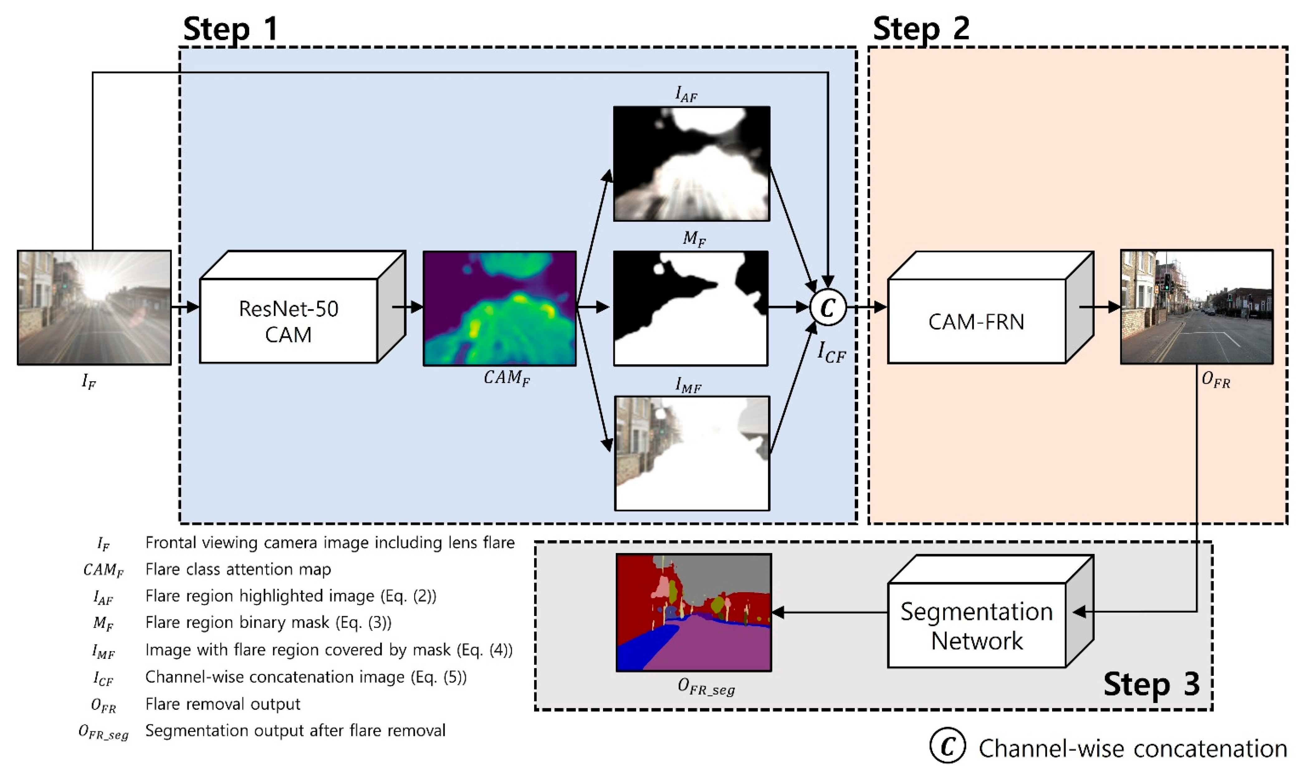
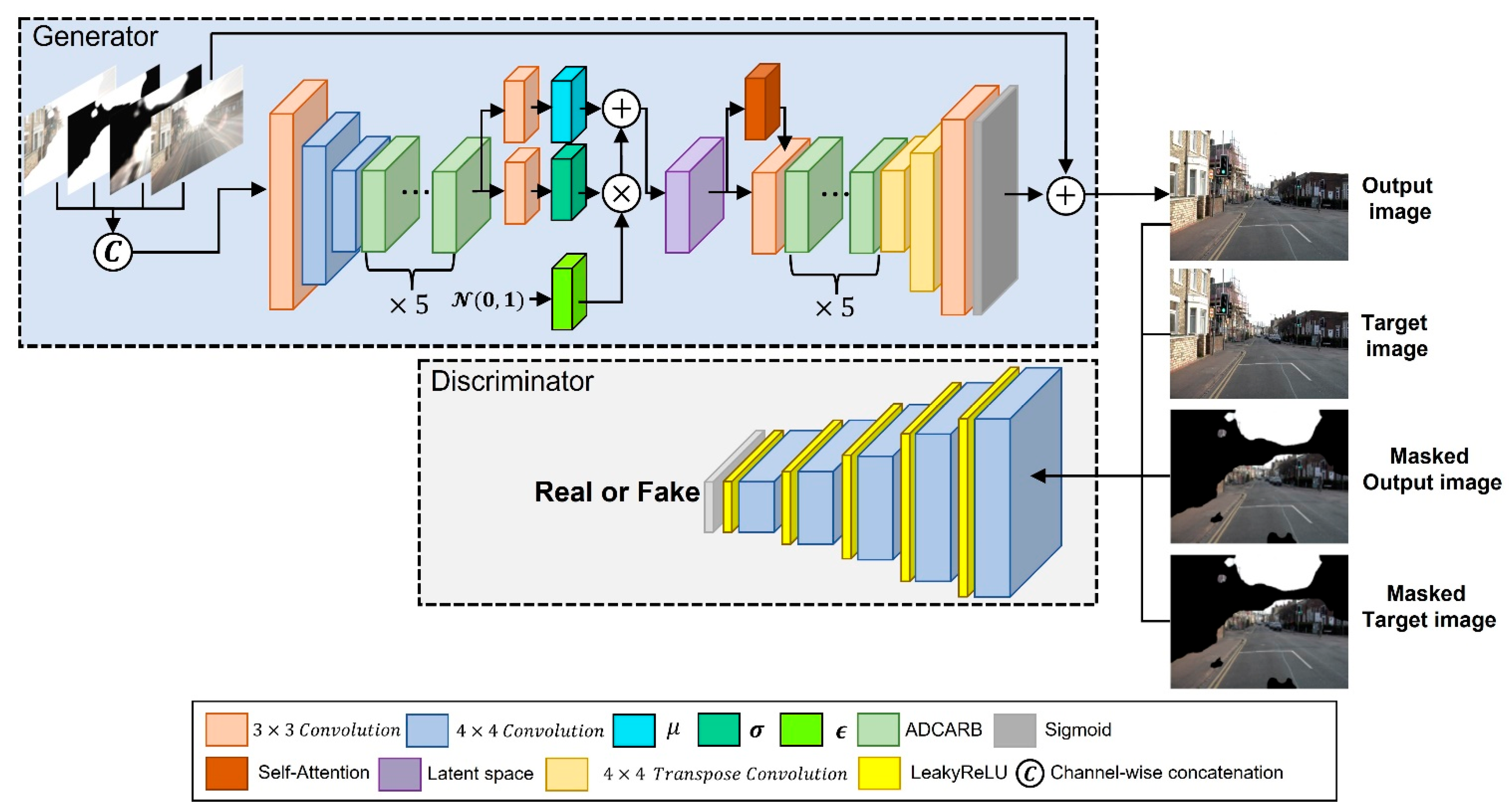
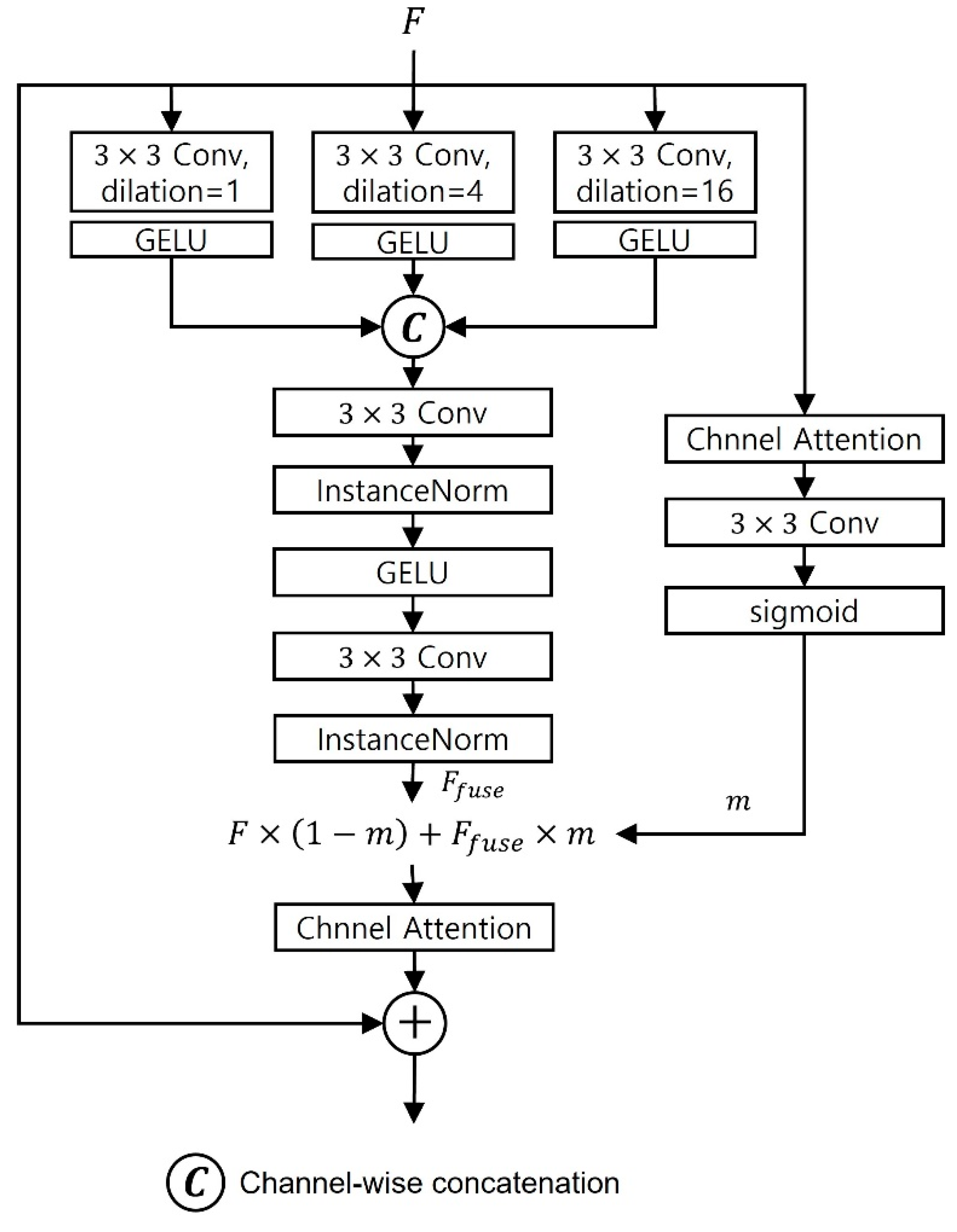
We compared the performance of CAM-FRN by combining the modules proposed in Section 3. We compared the semantic segmentation performance and image restoration performance by applying and not applying the following modules: a module for obtaining additional images using Equations (2)–(4) besides images damaged by a lens flare through CAM that represents the lens flare region in an image. Lastly, the ADCARB module, a self-attention module, fuses latent spaces that have undergone variational inference and applied with self-attention and not applied with self-attention, and sends them to the decoder. If ADCARB is not applied, the residual block used in the existing CycleGAN was applied; if the self-attention module is not applied, the latent space that has been sampled through variational inference is directly sent to the decoder. When the CAM module is not applied, the process of reflecting the mask for the lens flare region, which can be obtained by CAM and additional inputs in the losses, is omitted.

To compare the performance of different module combinations on each dataset, we analyzed the restoration performance with the results shown in

Table 6. Performance evaluation metrics of the restoration results for the images in which a lens flare is removed for the syn-flare CamVid dataset.

Modules			CamVid (2-Fold)
CAM	ADCARB	Self-Attention	PSNR	SSIM	FID
			16.83	0.7558	268.22
√			17.88	0.7775	227.49
	√		21.77	0.8650	49.27
		√	19.80	0.8163	150.81
√	√		26.66	0.9242	39.55
√		√	20.87	0.8361	136.94
	√	√	22.01	0.8706	42.96
√	√	√	27.95	0.9290	36.41

and

Table 7. Performance evaluation metrics of the restoration results for the images in which a lens flare is removed for the syn-flare KITTI dataset.

Modules			KITTI (2-Fold)
CAM	ADCARB	Self-Attention	PSNR	SSIM	FID
			15.70	0.7077	221.58
√			16.37	0.6519	251.58
	√		22.42	0.8441	52.84
		√	16.12	0.6963	229.38
√	√		25.49	0.9037	42.37
√		√	16.66	0.6950	241.91
	√	√	22.58	0.8445	47.87
√	√	√	26.04	0.9054	38.96

. Table 6 and Table 7 demonstrate the greatest performance improvement, and the best performance was exhibited for all metrics.

Consequently, we verified two aspects through the ablation study. First, inputs additionally obtained by CAM enabled ADCARB of CAM-FRN to utilize the additional information of flare sufficiently and efficiently. CAM provides additional information about the flare region, which highlights the flare-damaged areas within the feature. This enables ADCARB to effectively extract and restore damaged areas. The evidence for this is as follows: in an ablation study, applying ADCARB and self-attention alone without using CAM resulted in worse performance than applying CAM and ADCARB together. Second, it was experimentally proven that using CAM, ADCARB, and self-attention module together may be effective for posterior distribution inference for restoring clean images.

Next, we input the restored images into the segmentation network and tested them according to the combination of modules. To compare the performance with respect to the combination of the modules, the evaluation metrics of the semantic segmentation performance according to the combination of modules are shown in

Table 8. Performance evaluation metrics of the semantic segmentation test results for the images in which a lens flare is removed for the syn-flare CamVid dataset (unit: %).

Modules			CamVid (2-Fold)
CAM	ADCARB	Self-Attention	Class Acc	Pixel Acc	mIoU
			48.18	83.98	46.21
√			49.67	85.92	48.72
	√		66.20	93.92	69.87
		√	54.67	88.69	55.35
√	√		67.18	94.25	71.02
√		√	56.66	89.61	58.08
	√	√	66.78	94.19	70.54
√	√	√	67.34	94.33	71.26

and

Table 9. This table presents the performance evaluation metrics of the semantic segmentation test results for the images in which a lens flare is removed for the syn-flare KITTI dataset (unit: %).

Modules			KITTI (2-Fold)
CAM	ADCARB	Self-Attention	Class Acc	Pixel Acc	mIoU
			40.16	75.65	40.88
√			29.87	65.22	28.35
	√		53.57	89.67	58.46
		√	37.10	73.69	37.11
√	√		54.12	90.22	59.40
√		√	33.52	70.58	32.81
	√	√	53.78	89.84	58.68
√	√	√	54.73	90.62	60.27

.

Table 8 and Table 9 demonstrate the greatest performance improvement; the best performance was exhibited for all metrics. Accordingly, the metrics of object detection performance of semantic segmentation increase along with the restoration performance evaluation metrics according to the combination of modules.

Table 10. IoU performance evaluation metrics by class for the semantic segmentation test results of the images in which a lens flare is removed for the syn-flare CamVid dataset (unit: %).

Modules			CamVid (2-Fold)
CAM	ADCARB	Self-Attention	Sky	Building	Pole	Road	Pavement	Tree	Sign Symbol	Fence	Car	Pedestrian	Bicyclist	Average
			87.79	68.20	26.53	82.50	44.63	56.74	31.29	35.85	49.95	11.40	13.42	46.21
√			89.24	71.52	28.43	84.73	46.61	59.25	33.60	38.98	56.53	13.04	13.95	48.72
	√		92.81	84.51	44.42	95.66	78.64	74.95	53.95	57.81	82.65	49.06	54.06	69.87
		√	89.80	76.13	32.89	88.95	57.02	62.58	39.78	45.92	66.69	24.26	24.81	55.35
√	√		92.84	85.26	45.73	96.14	80.31	75.70	55.48	59.08	83.59	51.17	55.96	71.02
√		√	90.53	77.34	35.01	90.09	59.45	64.07	42.52	47.25	71.68	28.56	32.41	58.08
	√	√	92.96	85.25	45.28	95.97	79.86	75.33	55.20	59.00	83.02	50.86	53.24	70.54
√	√	√	92.94	85.39	45.90	96.24	80.54	76.03	56.10	59.92	83.74	51.58	55.49	71.26

and

Table 11. This table presents the IoU of each class for the semantic segmentation test results of the images in which a lens flare is removed for the syn-flare KITTI dataset (unit: %).

Modules			KITTI (2-Fold)
CAM	ADCARB	Self-Attention	Sky	Building	Pole	Road	Pavement	Tree	Sign Symbol	Fence	Car	Pedestrian	Bicyclist	Average
			62.23	51.26	21.68	65.90	41.59	60.73	36.94	26.41	52.91	15.35	14.75	40.88
√			42.91	44.31	16.33	38.64	23.34	53.99	28.02	18.11	29.82	7.24	4.12	28.35
	√		73.84	73.68	33.01	87.72	64.34	81.66	50.05	42.21	75.73	28.19	32.71	58.46
		√	53.45	50.26	21.22	58.15	35.63	61.37	35.77	24.32	48.45	11.20	8.36	37.11
√	√		74.59	74.53	33.78	88.60	65.59	82.78	50.31	42.07	76.34	30.72	34.03	59.40
√		√	41.53	46.92	16.56	58.56	34.08	57.31	25.93	20.54	44.22	6.98	8.26	32.81
	√	√	74.27	73.94	33.39	87.98	64.95	82.15	49.83	41.75	75.37	28.63	33.23	58.68
√	√	√	74.43	75.93	33.87	89.02	66.69	83.21	50.50	43.14	77.50	31.92	36.78	60.27

present IoU metrics per class in which IoU metrics of each class were improved according to the restoration performance evaluation metrics, as analyzed in Table 8 and Table 9.

Next, we conducted an ablation study for numerically analyzing the semantic segmentation performance for the combination of inputs created with CAM. As shown in

Table 12. Comparison of the semantic segmentation performance for the combination of additional inputs obtained from CAM for syn-flare CamVid dataset (unit: %).

Additional Inputs				CamVid (2-Fold)
${\mathit{I}}_{\mathit{F}}$	${\mathit{I}}_{\mathit{A}\mathit{F}}$	${\mathit{M}}_{\mathit{F}}$	${\mathit{I}}_{\mathit{M}\mathit{F}}$	Class Acc	Pixel Acc	mIoU
√				67.26	94.33	71.13
√	√			67.25	94.29	71.12
√		√		67.24	94.26	71.06
√			√	67.17	94.32	71.09
√	√	√		67.32	94.32	71.23
√		√	√	67.12	94.29	71.05
√	√		√	67.11	94.32	71.15
√	√	√	√	67.34	94.33	71.26

and

Table 13. Comparison of the semantic segmentation performance for the combination of additional inputs obtained from CAM for syn-flare KITTI dataset (unit: %).

Additional Inputs				KITTI (2-Fold)
${\mathit{I}}_{\mathit{F}}$	${\mathit{I}}_{\mathit{A}\mathit{F}}$	${\mathit{M}}_{\mathit{F}}$	${\mathit{I}}_{\mathit{M}\mathit{F}}$	Class Acc	Pixel Acc	mIoU
√				54.70	90.71	60.06
√	√			54.69	90.55	59.95
√		√		54.52	90.46	59.85
√			√	54.69	90.64	60.12
√	√	√		54.54	90.69	60.06
√		√	√	54.70	90.54	60.11
√	√		√	54.64	90.62	60.15
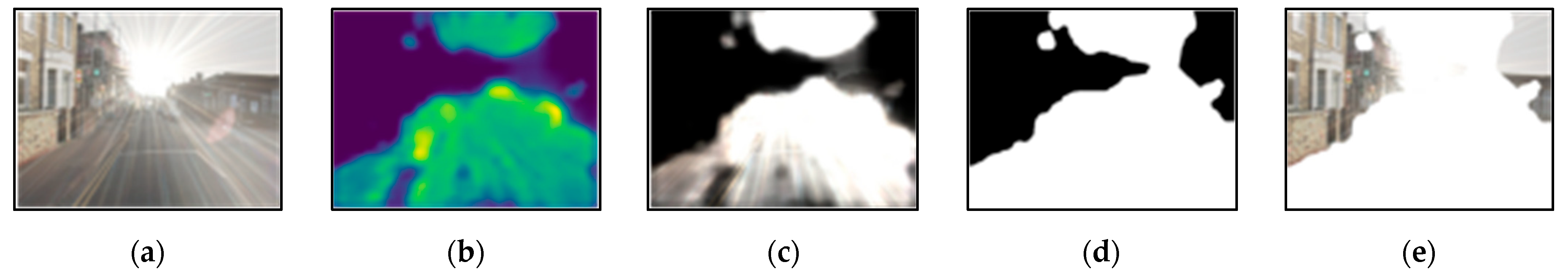
√	√	√	√	54.73	90.62	60.27

, we measured the semantic segmentation performance according to the combination of additional inputs based on class accuracy, pixel accuracy, and mIoU. An image $I_F$ damaged by a flare was used in all combinations as a default, and we compared the performance of the combinations when the inputs proposed in our method were all used and unused.

According to Table 12, there was no significant difference in the performance according to the combination of inputs. However, class accuracy, pixel accuracy, and mIoU were the highest when all inputs were used, as we proposed. In particular, when mIoU was increased by 0.13% then when only $I_F$ was used, and mIoU was 0.03% higher than the combination of $I_F$, $I_{AF}$, and $M_F$ which demonstrated the second highest mIoU. And Table 13 similarly shows that there is no significant difference in performance based on the combination of inputs. However, as suggested, using all inputs resulted in the highest-class accuracy, pixel accuracy, and mIoU. Specifically, mIoU was 0.21% higher than using $I_F$ alone and 0.12% higher than the combination of $I_F$, $I_{AF}$, and $I_{MF}$.

(b)

Performance Comparisons with and without Variational Inference

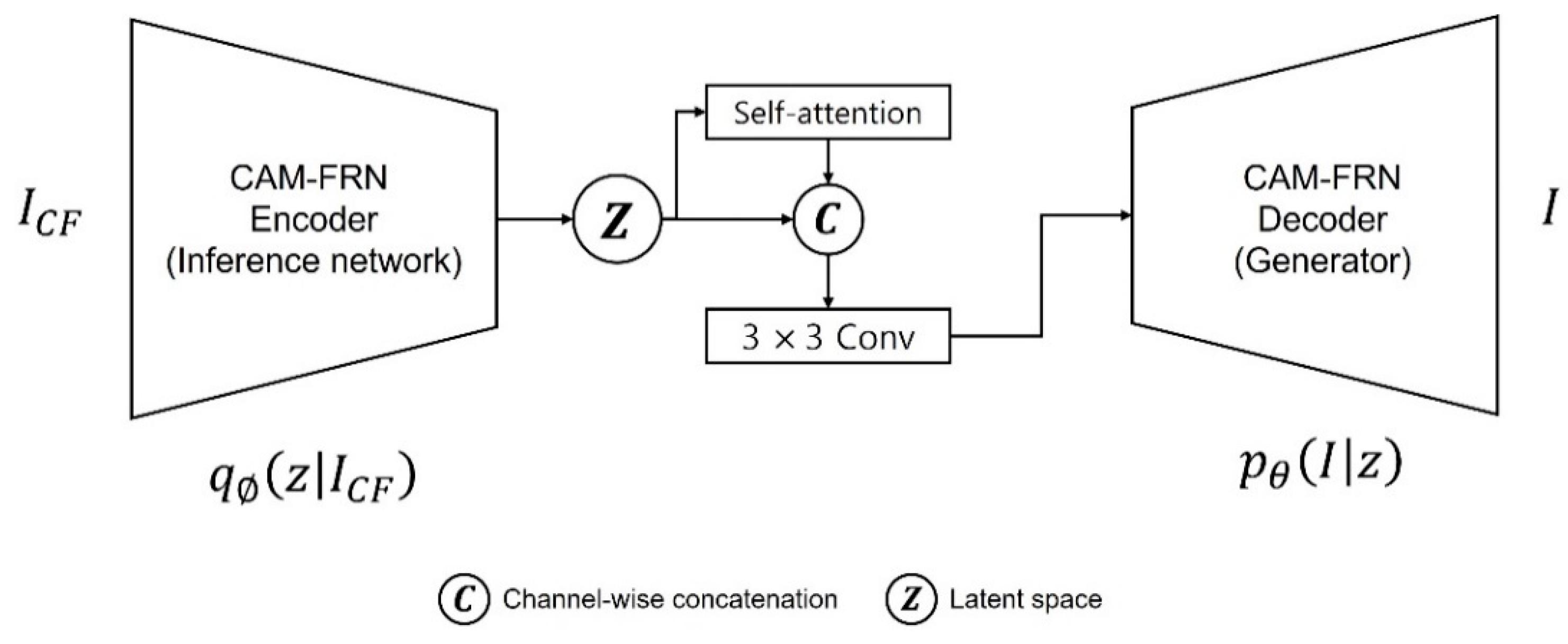
In this section, we conducted an ablation study to verify the effects of adopting variational inference on the performance of our proposed method. The reparameterization trick structure for variational inference was removed between the encoder and decoder of CAM-FRN; then, latent spaces from the encoder that were applied with self-attention and not applied with self-attention were fused to be delivered to the decoder. Additionally, the experiment was conducted using L1 loss and L2 loss, without using the Kullback–Leibler divergence (KL divergence), which was applied to reduce the difference between true posterior distribution and posterior distribution inferred by the inference network, or the reconstruction loss used for variational inference.

Table 14. Comparison of the restoration performance when variational inference is used and when L1 and L2 losses replace variational inference for syn-flare CamVid dataset.

Loss	CamVid (2-Fold)
	PSNR	SSIM	FID
w/o variational inference, use L1 loss	27.58	0.9238	50.76
w/o variational inference, use L2 loss	26.41	0.9188	51.63
w variational inference	27.95	0.9290	36.41

and

Table 15. This table compares the restoration performance when variational inference is used and when L1 and L2 losses replace variational inference for syn-flare KITTI dataset.

Loss	KITTI (2-Fold)
	PSNR	SSIM	FID
w/o variational inference, use L1 loss	25.58	0.9070	55.23
w/o variational inference, use L2 loss	24.61	0.9014	60.09
w variational inference	26.04	0.9054	38.96

present the evaluation metrics of the restoration performance for syn-flare CamVid dataset and syn-flare KITTI dataset. When L1 loss was used in place of variational inference, both datasets showed PSNR and SSIM did not exhibit a noticeable performance difference, but the FID score exhibited a significant difference. The FID score is a metric for evaluating the quality of images generated by the GAN structure, which uses a discriminator to calculate the distance between the distribution of the generated image and the distribution of the ground-truth image. The reason for using variational inference was to generate images that were semantically similar to the ground-truth image as much as possible in the decoder by sampling a significant latent space through the inference of the posterior distribution, which considered the ground-truth image. In other words, we aim to minimize the difference between the inferred posterior distribution $q_{\mathrm{\varnothing }}\left(z|I_{CF}\right)$ and the true posterior distribution $p\left(z|I\right)$ as shown in Equation (16). Therefore, Table 14 and Table 15 show that using variational inference can result in a better performance in terms of the FID score.

When L2 loss is used instead of variant inference, similar results are yielded to the analysis using L1 loss when compared with using variant inference. Similarly, the FID score was significantly reduced when using variant inference, and as discussed above, using variant inference can lead to better performance in terms of FID score.

As shown in

Table 16. Comparison of the semantic segmentation performance when variational inference is used and when L1 and L2 losses replace variational inference for syn-flare CamVid dataset (unit: %).

Loss	CamVid (2-Fold)
	Class Acc	Pixel Acc	mIoU
w/o variational inference, use L1 loss	65.92	93.74	69.48
w/o variational inference, use L2 loss	65.99	93.73	69.38
w variational inference	67.34	94.33	71.26

and

Table 17. This table compares the semantic segmentation performance for the restored images when variational inference is used and when L1 and L2 losses replace variational inference for syn-flare KITTI dataset (unit: %).

Loss	KITTI (2-Fold)
	Class Acc	Pixel Acc	mIoU
w/o variational inference, use L1 loss	52.78	89.29	57.71
w/o variational inference, use L2 loss	52.83	89.39	57.80
w variational inference	54.73	90.62	60.27

, the same performance improvements in semantic segmentation were demonstrated in restoration. We can see that class accuracy, pixel accuracy, and mIoU are highest when using variational inference.

(c)

Performance Comparisons According to Mask Considering Loss

For the next comparative experiment, we evaluate the semantic segmentation performance and image restoration performance for the two cases of considering the flare region and not considering the flare region in the proposed loss equation. For image-to-image translation, we used content loss [42] and style loss [42] based on VGG-19. Content loss and style loss were applied to the result of multiplying a flare region mask to the final output image and to the ground-truth image. Furthermore, the lens flare region was considered for the losses utilizing a discriminator; the image restoration performance was improved by making it difficult for the discriminator to discriminate whether the flare region is ground truth by focusing on the flare region. Accordingly, we expected CAM-FRN to concentrate more on the flare region for removal. We experimentally proved that our hypothesis is valid, as shown in

Table 18. Comparison of the restoration performance when a mask is considered and not considered in the loss for syn-flare CamVid dataset.

Loss	CamVid (2-Fold)
	PSNR	SSIM	FID
w/o mask	21.96	0.8686	44.48
w mask	27.95	0.9290	36.41

,

Table 19. This table compares the restoration performance when a mask is considered and not considered in the loss for syn-flare KITTI dataset.

Loss	KITTI (2-Fold)
	PSNR	SSIM	FID
w/o mask	21.68	0.8483	61.78
w mask	26.04	0.9054	38.96

,

Table 20. Comparison of the semantic segmentation test performance when a mask is considered and not considered in the loss for syn-flare CamVid dataset (unit: %).

Loss	CamVid (2-Fold)
	Class Acc	Pixel Acc	mIoU
w/o mask	66.38	94.09	70.16
w mask	67.34	94.33	71.26

and

Table 21. This table compares the semantic segmentation test performance when a mask is considered and not considered in the loss for syn-flare KITTI dataset (unit: %).

Loss	KITTI (2-Fold)
	Class Acc	Pixel Acc	mIoU
w/o mask	52.46	88.75	57.26
w mask	54.73	90.62	60.27

.

Table 18 and Table 19 are analyzed with respect to the restoration results. When the loss considering a mask is used, PSNR and SSIM were improved, respectively, compared with when not used. Further, the FID score was also significantly decreased. These results demonstrate that considering the lens flare region and the entire image together significantly improves performance. Segmentation performance was also improved along with the restoration performance. According to Table 20 and Table 21, when the loss considering a mask was used, class accuracy, pixel accuracy, and mIoU all increased, respectively, compared with when not used.

(2)

Comparisons of Proposed Method and the State-of-the-Art Methods

We compared our proposed lens flare removal method with the previously proposed methods of Qiao et al. [23] and Wu et al. [9]. However, research has been insufficiently conducted owing to the difficulties of a lens flare removal task. Therefore, we additionally adopted several networks that were similar to our research purpose to compare the performance.

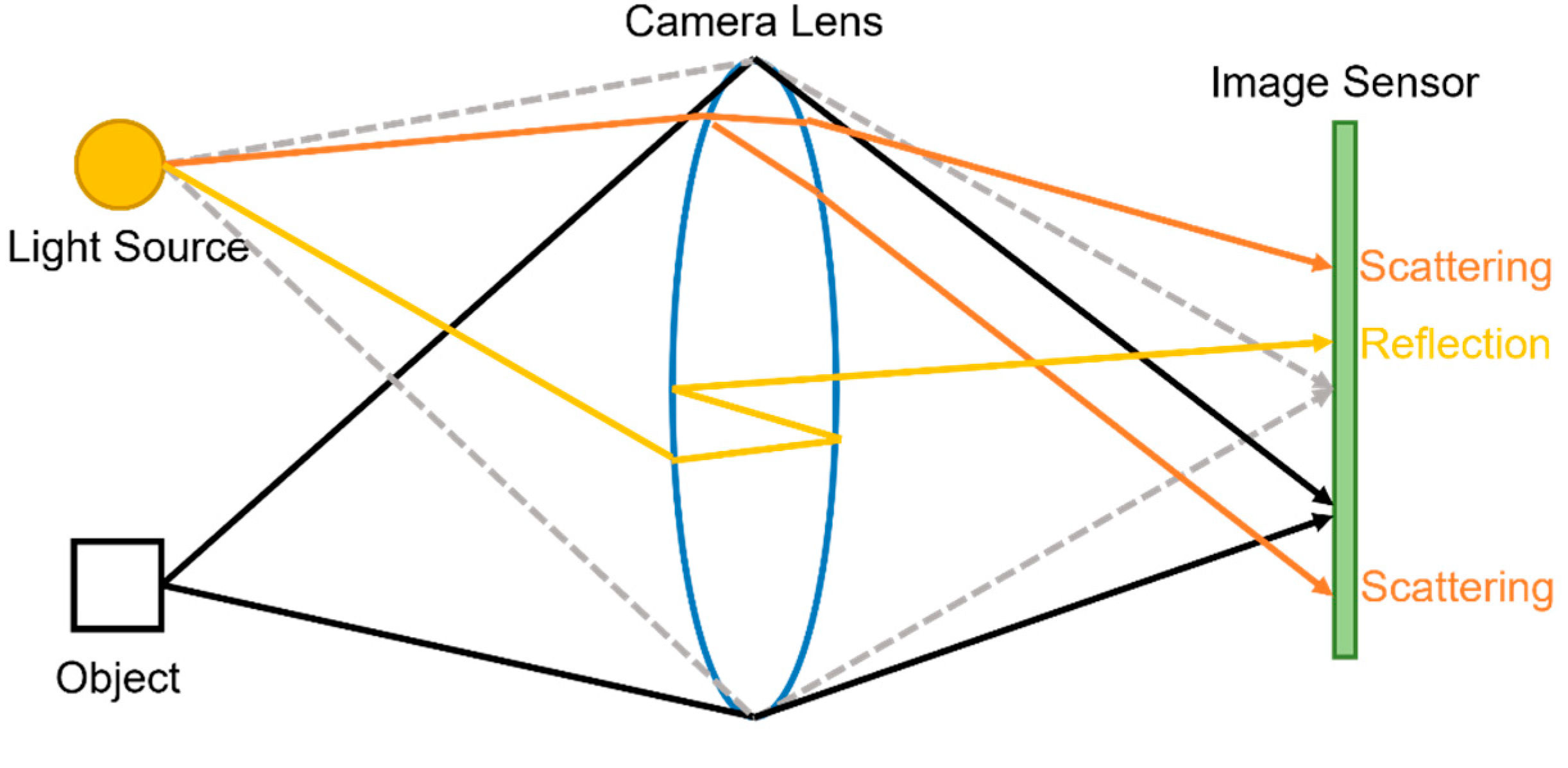
The proposed method used a GAN-based learning method utilizing a discriminator, wherein an image with a flare undergoes image-to-image translation to a clean image without flare. Therefore, we compared our proposed model with Pix2Pix [37] and CycleGAN [50], which have been commonly proposed for image-to-image translation. Lastly, we compared the performance against FFANet [22] and MPRNet [21] proposed for dehazing and deraining, respectively. Dehazing and deraining tasks aim to remove artifacts covering the objects in an image owing to environmental factors, which are similar to the lens flare removal task, which removes artifacts generated in the presence of a strong light source in the surrounding. In particular, hazing was similar to a lens flare artifact generated by light scattering, and veiling glare, which affects contrast within an image and causes the image to become hazy; therefore, we compare our proposed method with the networks designed for dehazing considering they were deemed effective in removing lens flare artifacts. Raining was similar to light streaks that radiated from a light source among various lens flare artifacts. We compared our proposed method with MPRNet, which was considered effective in restoring the image details covered by light streaks. 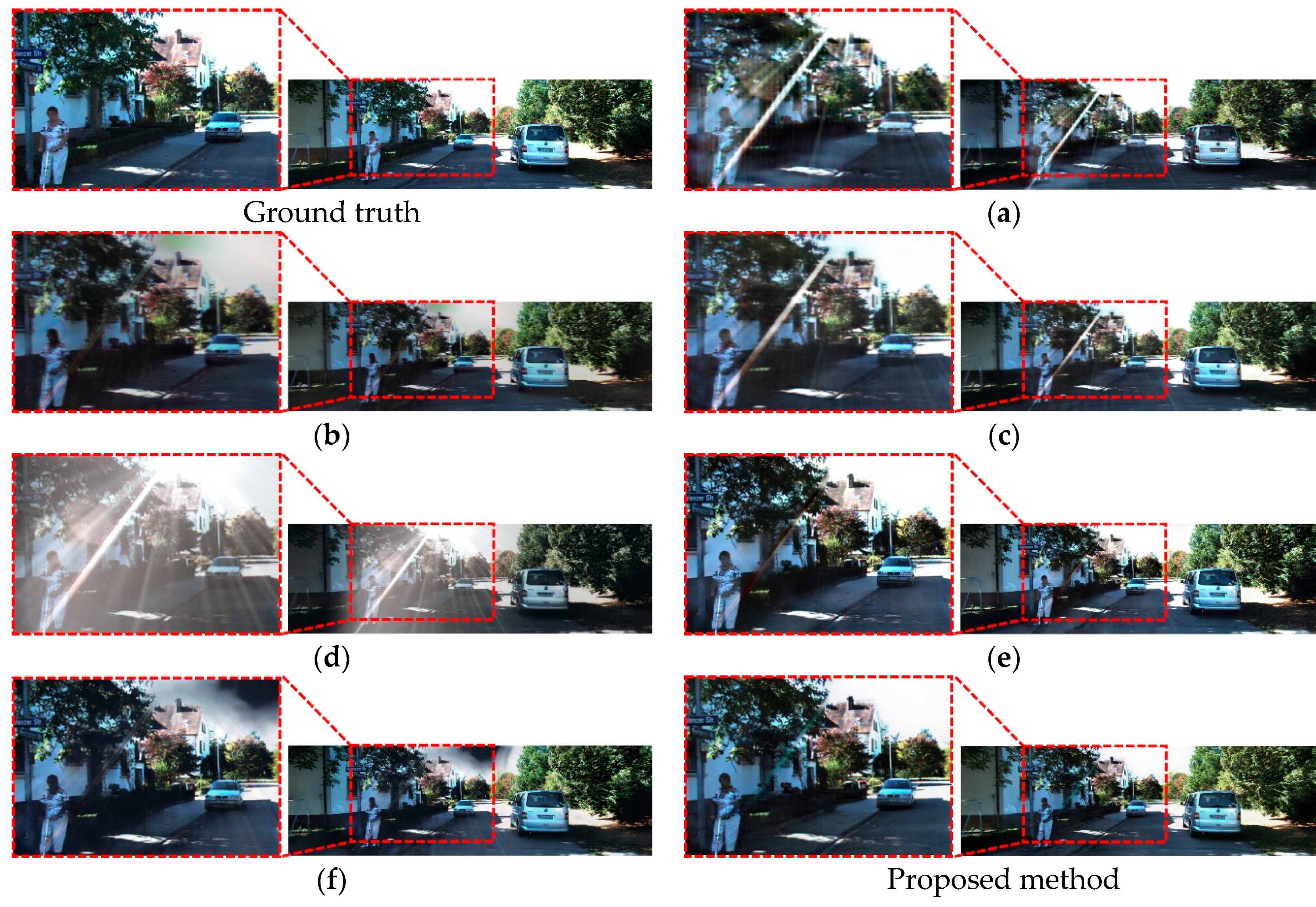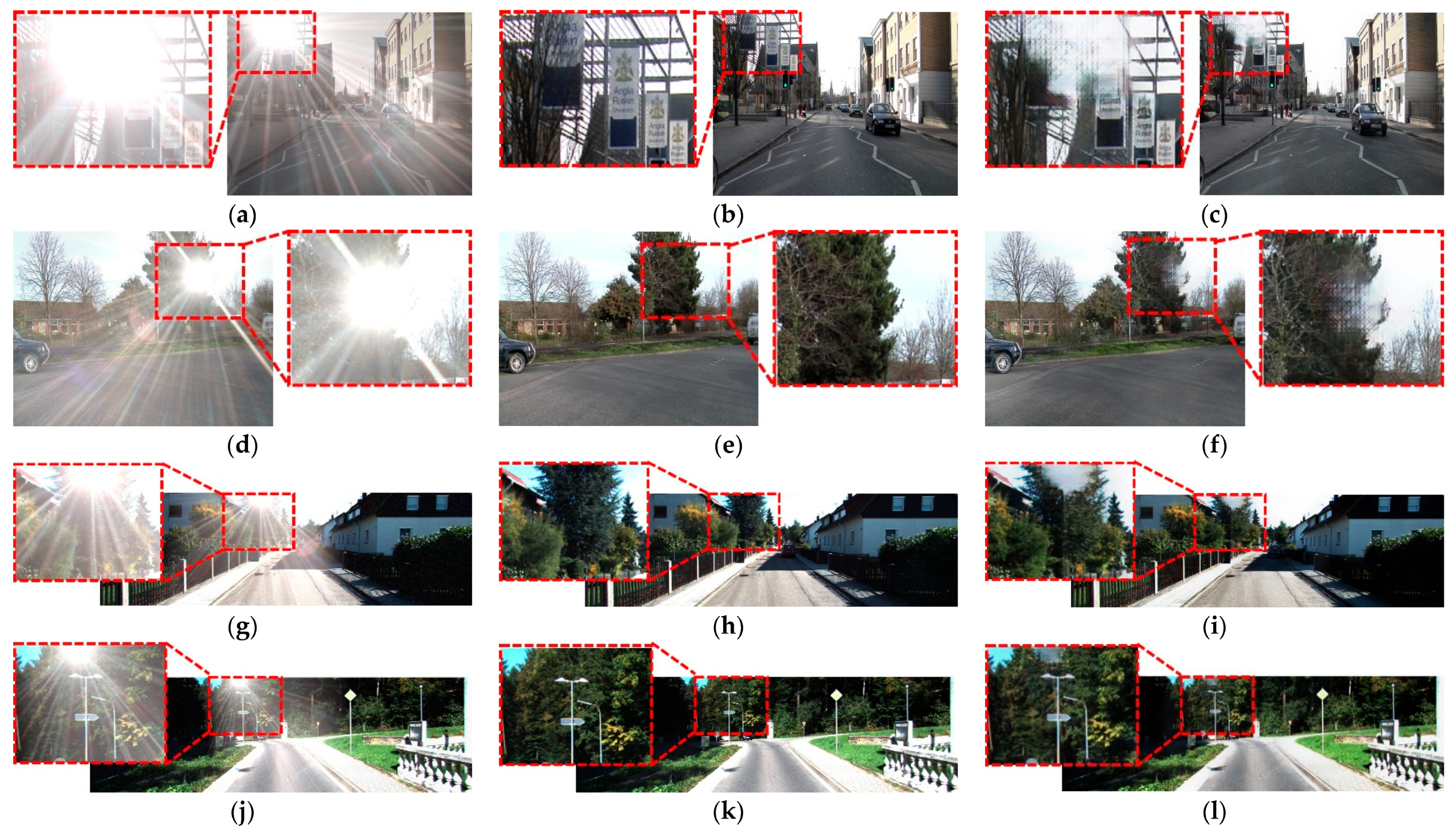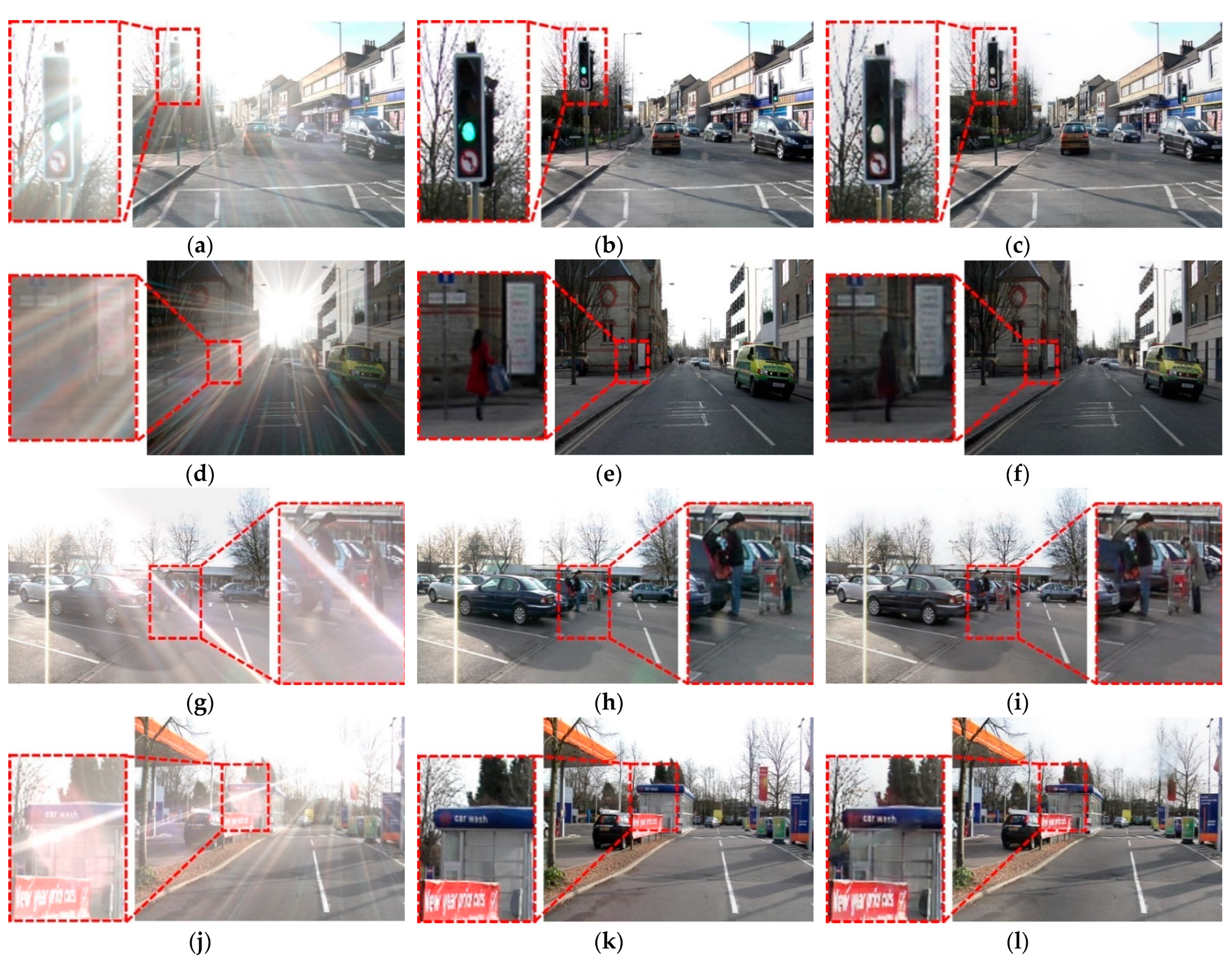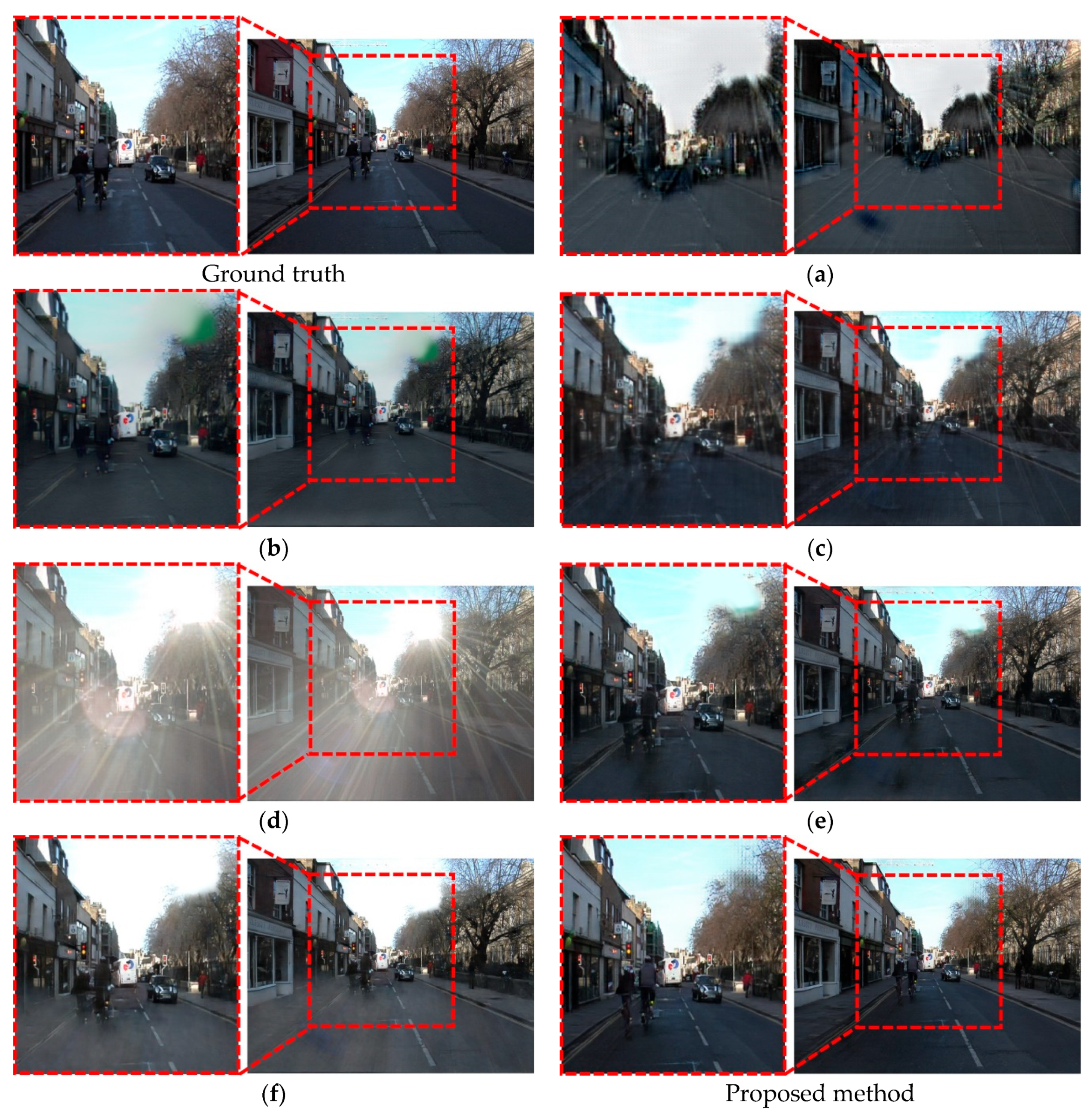Figure 11 and Figure 12 show the restoration results of the proposed method and previously explained methods.

The method proposed by Qiao et al. [23] effectively removes reflection artifacts where the flare region is seen; however, their method was proven ineffective in removing lens flare artifacts generated through the image. As shown in Figure 11a and Figure 12a, large regions of a flare within the image were not effectively removed throughout the image, and the restoration result was poorer than our proposed method. The method proposed by Wu et al. [9] demonstrated a better performance than [23]; however, lens flare was not completely removed. As shown in Figure 11b, this method could not restore the details of the boundary between the road and sidewalk, or the details of people riding a bicycle. And in Figure 12b, the artifacts overlaid on the pedestrian are not completely removed.

Next, we analyzed the restoration results of Pix2Pix and CycleGAN, which were proposed for image-to-image translation. Pix2Pix was far more outstanding than CycleGAN, considering the translation and execution from flare image to clean image and vice versa was not sufficiently trained. Conversely, the restoration results of Pix2Pix were visually more outstanding where the conditions of the ground-truth image were directly given to the discriminator. Compared with the proposed CAM-FRN, the restoration results of Pix2Pix did not adequately restore the details of the boundary between road and sidewalk, and light streaks of flare were remaining.

Lastly, our proposed method was compared with FFANet and MPRNet proposed for dehazing and deraining, respectively. Compared with the previously compared models, these models demonstrated a far more outstanding performance visually. MPRNet was effective in removing light streaks; however, it did not accurately restore the details of roads. FFANet successfully restored the image that became hazy by a flare to a clean original image, but flare artifacts were not perfectly removed. In contrast, our proposed method successfully restored the details of roads while adequately removing flare artifacts with outstanding performance.

Table 22. Comparison of the restoration performance of the proposed method and state-of-the-art methods for syn-flare CamVid dataset.

Method	CamVid (2-Fold)
	PSNR	SSIM	FID
Qiao et al. [23]	17.53	0.6020	238.20
Wu et al. [9]	19.17	0.8174	104.97
Pix2Pix [37]	24.78	0.8685	139.10
CycleGAN [50]	13.53	0.6613	309.68
FFANet [22]	27.61	0.9178	77.88
MPRNet [21]	23.48	0.8842	125.03
Proposed	27.95	0.9290	36.41

and

Table 23. This table compares the restoration performance of the proposed method and state-of-the-art methods for syn-flare KITTI dataset.

Method	KITTI (2-Fold)
	PSNR	SSIM	FID
Qiao et al. [23]	18.58	0.7121	192.92
Wu et al. [9]	19.89	0.7543	86.52
Pix2Pix [37]	22.66	0.8314	119.59
CycleGAN [50]	14.07	0.6571	238.81
FFANet [22]	25.64	0.9048	72.13
MPRNet [21]	22.43	0.8715	120.41
Proposed	26.04	0.9054	38.96

present the numerical performance evaluation metrics according to the results of restoring images synthesized with a lens flare of each method. Among various models, the PSNR, SSIM, and FID scores of our proposed model were the best. FFANet demonstrated the second-highest performance, where PSNR and SSIM were similar to our method; however, the FID score was approximately 30 points higher than our proposed method. Based on such results, the distance difference of the feature maps extracted from inception v3 network [49] was smaller in the proposed CAM-FRN than FFANet, and the result image was closer to the ground-truth image.

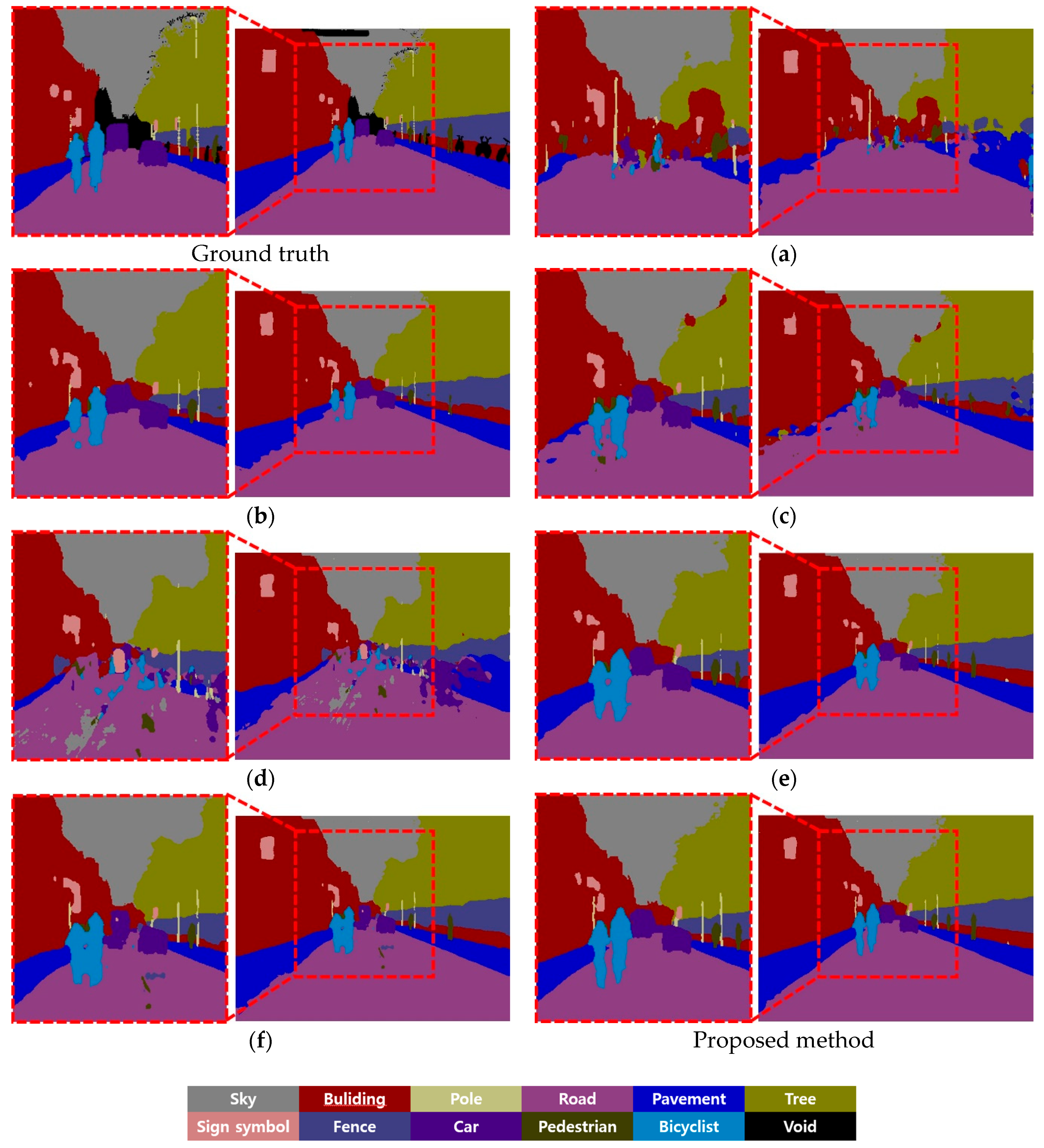
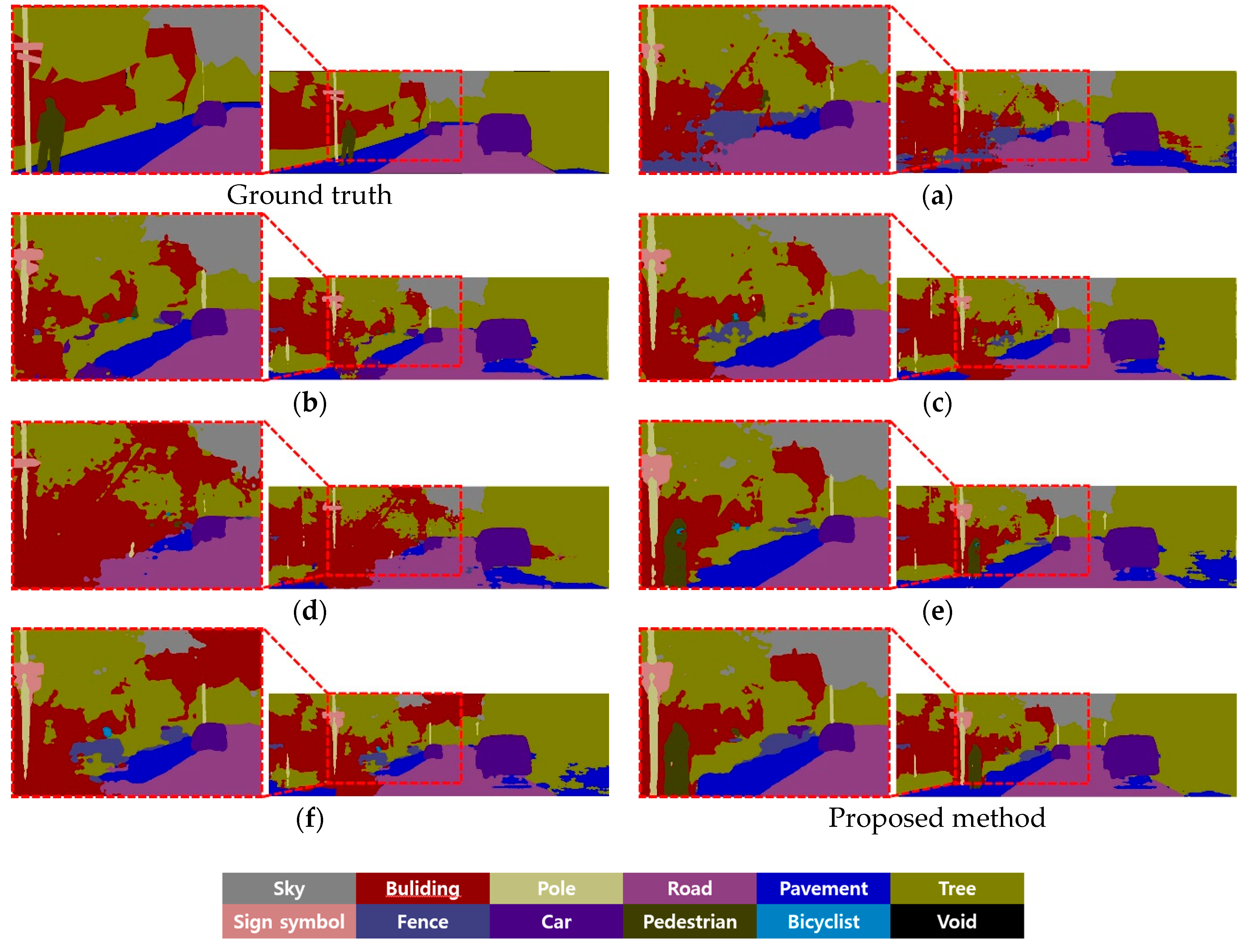
Figure 13 and Figure 14 show the semantic segmentation test results for the images restored by our proposed method, the previously proposed method for flare removal, image-to-image translation methods, and the methods for dehazing and deraining. Overall, segmentation performance improved tremendously as the restoration performance improved. The method proposed by Qiao et al. [23] was ineffective in removing lens flare artifacts generated throughout the image, as in the restoration result, thus also exhibiting poor segmentation results. The method proposed by Wu et al. [9] effectively removed lens flare artifacts generated through the image compared with the method proposed in [23], but as shown in the segmentation results in Figure 13b, the details of the road, sidewalk boundary, and the person riding the bike were not properly restored, which contradicts the restoration results in Figure 11b, and the pedestrian was not detected at all in Figure 14b.

Next, the segmentation test results were analyzed according to the restoration result of Pix2Pix and CycleGAN, which were proposed for image-to-image translation. The restoration result of Pix2Pix was more outstanding than that of CycleGAN; which is in line with the restoration result, and the segmentation test result of the image restored by Pix2Pix was more outstanding than CycleGAN. However, Pix2Pix could not remove lens flare artifacts perfectly; road or people riding a bicycle were not properly detected depending on the restoration results, as shown in the enlarged part in Figure 13 and Figure 14.

Lastly, we compared the segmentation performance of FFANet and MPRNet. The segmentation result of the images restored by FFANet in Figure 13e and Figure 14e, visually showed a greater segmentation improvement compared with (a)–(d), which are the results of the previous methods. As presented in

Table 24. This table compares the semantic segmentation performance of the images restored by the proposed method and state-of-the-art methods for syn-flare CamVid dataset (unit: %).

Method	CamVid (2-Fold)
	Class Acc	Pixel Acc	mIoU
Qiao et al. [23]	39.53	79.24	36.26
Wu et al. [9]	59.98	90.54	61.19
Pix2Pix [37]	54.79	88.71	54.70
CycleGAN [50]	43.82	80.95	40.95
FFANet [22]	65.01	92.81	67.73
MPRNet [21]	60.85	91.34	62.35
Proposed	67.34	94.33	71.26

and

Table 25. This table compares the semantic segmentation performance of the images restored by the proposed method and state-of-the-art methods for syn-flare KITTI dataset (unit: %).

Method	KITTI (2-Fold)
	Class Acc	Pixel Acc	mIoU
Qiao et al. [23]	36.28	68.20	34.49
Wu et al. [9]	46.96	84.23	48.33
Pix2Pix [37]	44.33	81.41	44.95
CycleGAN [50]	34.92	70.01	34.25
FFANet [22]	52.98	89.17	57.57
MPRNet [21]	49.42	85.99	52.97
Proposed	54.73	90.62	60.27

, the class accuracy, pixel accuracy, and mIoU were lower than that of the proposed method. Additionally, as shown in the enlarged part in Figure 13e, the proposed method detected the shape of a bicyclist object more effectively compared with other methods. When the pedestrian class in the enlarged part of Figure 14e and the enlarged part of the proposed method are compared, the proposed method detected the shape of the pedestrian more effectively. The segmentation result of the images restored by MPRNet in Figure 13f demonstrated a noticeable performance improvement compared with other methods, as in Figure 14e; however, the class accuracy, pixel accuracy, and mIoU were 6.49%, 2.99%, and 8.91% lower than that of the proposed method. In the segmentation result of the image restored by MPRNet shown in Figure 14f, the pedestrian was not detected at all. Class accuracy, pixel accuracy, and mIoU are 5.31%, 4.63%, and 7.3% lower than the proposed method, respectively.

Table 26. Comparisons of the proposed and the state-of-the-art methods for syn-flare CamVid dataset (unit: %).

Method		CamVid (2-Fold)
		Sky	Building	Pole	Road	Pavement	Tree	Sign Symbol	Fence	Car	Pedestrian	Bicyclist	Average
Original	PSPNet [2]	88.65	83.97	10.23	96.22	79.43	74.78	40.68	61.49	74.98	36.66	46.59	63.06
	ICNet [3]	91.74	83.40	9.07	96.26	77.92	74.42	36.07	53.94	76.99	34.76	43.29	61.63
	CGNet [44]	92.21	83.55	18.27	96.85	79.58	75.02	37.10	52.25	79.11	38.95	43.02	63.26
	DeepLabV3+ [7]	93.67	88.50	52.44	97.46	85.40	80.23	64.51	67.96	87.58	64.50	65.94	77.11
Without restoration	PSPNet [2]	84.66	67.14	5.16	80.23	41.37	55.84	21.72	31.11	39.12	5.84	6.41	39.87
	ICNet [3]	85.46	61.84	4.05	75.51	33.53	51.11	10.27	23.05	26.28	2.35	3.38	34.36
	CGNet [44]	86.80	60.12	8.23	73.33	33.67	48.16	9.59	19.41	25.62	2.17	2.56	33.61
	DeepLabV3+ [7]	85.62	66.85	24.97	78.53	39.68	57.50	32.25	31.54	42.13	10.10	12.46	43.78
With restoration use DeepLabV3+	Qiao et al. [23]	86.28	61.54	14.39	78.95	32.01	47.43	12.25	21.91	33.97	6.87	3.78	36.26
	Wu et al. [9]	91.62	78.59	36.67	90.44	63.56	67.08	46.68	47.19	74.90	37.83	38.49	61.19
	Pix2Pix [37]	91.67	75.32	30.51	89.04	54.25	63.17	37.65	41.71	65.33	27.75	25.31	54.70
	CycleGAN [50]	84.79	64.03	21.85	77.59	37.11	54.67	25.31	29.54	38.94	8.13	8.54	40.95
	FFANet [22]	92.42	82.95	43.52	93.36	71.96	71.93	53.51	56.57	80.59	47.70	50.13	67.73
	MPRNet [21]	91.23	79.78	38.29	91.43	68.36	68.05	45.99	51.04	72.49	38.84	40.33	62.35
	Proposed	92.94	85.39	45.90	96.24	80.54	76.03	56.10	59.92	83.74	51.58	55.49	71.26

and

Table 27. Comparisons of proposed and the state-of-the-art methods for syn-flare KITTI dataset (unit: %).

Method		KITTI (2-Fold)
		Building	Sky	Pole	Road	Pavement	Tree	Sign Symbol	Fence	Car	Pedestrian	Bicyclist	Average
Original	PSPNet [2]	73.43	79.75	18.10	90.12	70.37	87.76	45.83	47.89	78.22	33.03	35.00	59.96
	ICNet [3]	73.48	76.49	12.01	88.48	64.71	86.37	34.48	38.60	72.84	11.80	20.96	52.75
	CGNet [44]	72.35	74.94	14.70	87.90	62.74	84.93	27.48	35.69	69.23	8.13	4.88	49.36
	DeepLabV3+ [7]	76.15	81.66	37.25	91.54	73.57	88.72	56.53	51.02	82.89	44.90	48.85	66.65
Without restoration	PSPNet [2]	50.83	50.98	12.07	61.65	48.98	56.10	31.04	29.70	48.34	9.87	7.49	37.00
	ICNet [3]	45.62	47.17	7.06	65.33	43.80	51.99	21.04	23.37	38.02	2.92	4.04	31.85
	CGNet [44]	40.62	42.41	7.42	63.67	42.51	47.58	15.35	21.73	29.12	1.81	1.55	28.52
	DeepLabV3+ [7]	60.47	51.57	25.72	74.20	51.81	59.45	39.94	32.45	55.70	15.81	16.53	43.97
With restoration use DeepLabV3+	Qiao et al. [23]	60.01	45.91	17.10	58.20	39.49	52.11	28.11	21.37	41.16	7.92	8.01	34.49
	Wu et al. [9]	68.46	67.04	24.32	73.34	53.47	73.99	41.56	32.68	62.76	16.74	17.22	48.33
	Pix2Pix [37]	68.41	62.14	22.01	70.36	51.86	70.01	36.54	28.85	56.94	12.74	14.61	44.95
	CycleGAN [50]	48.27	44.80	18.33	64.32	40.40	53.54	26.23	24.02	41.17	7.29	8.36	34.25
	FFANet [22]	73.08	73.81	32.41	85.79	61.65	81.01	49.14	41.06	74.55	26.08	34.69	57.57
	MPRNet [21]	67.81	67.07	30.52	80.93	56.82	75.84	46.23	37.88	67.60	23.89	28.12	52.97
	Proposed	74.43	75.93	33.87	89.02	66.69	83.21	50.50	43.14	77.50	31.92	36.78	60.27

present the IoU of each class in the semantic segmentation result of the images restored by each method. As analyzed above, the proposed method demonstrates the best performance in terms of IoU per class.

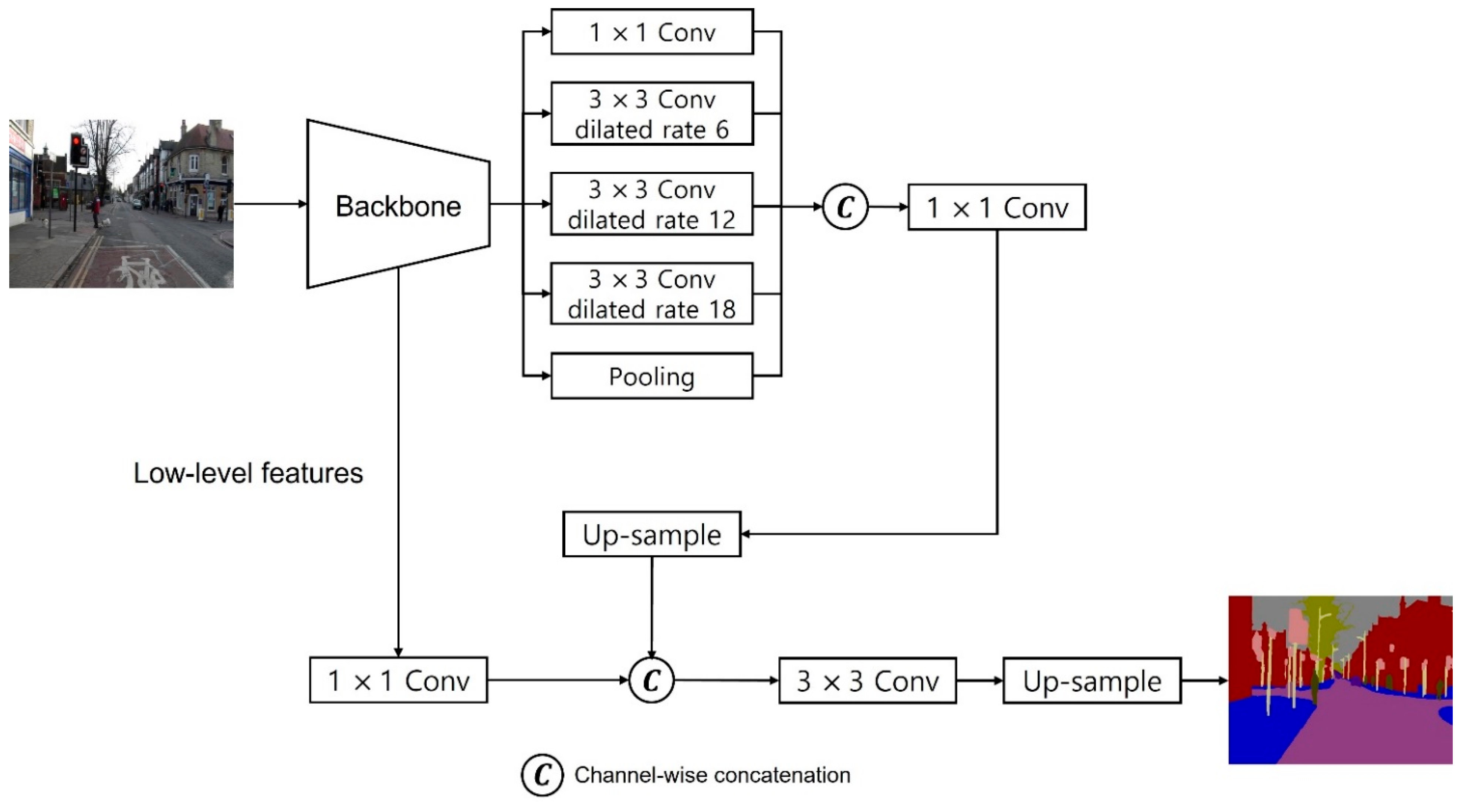
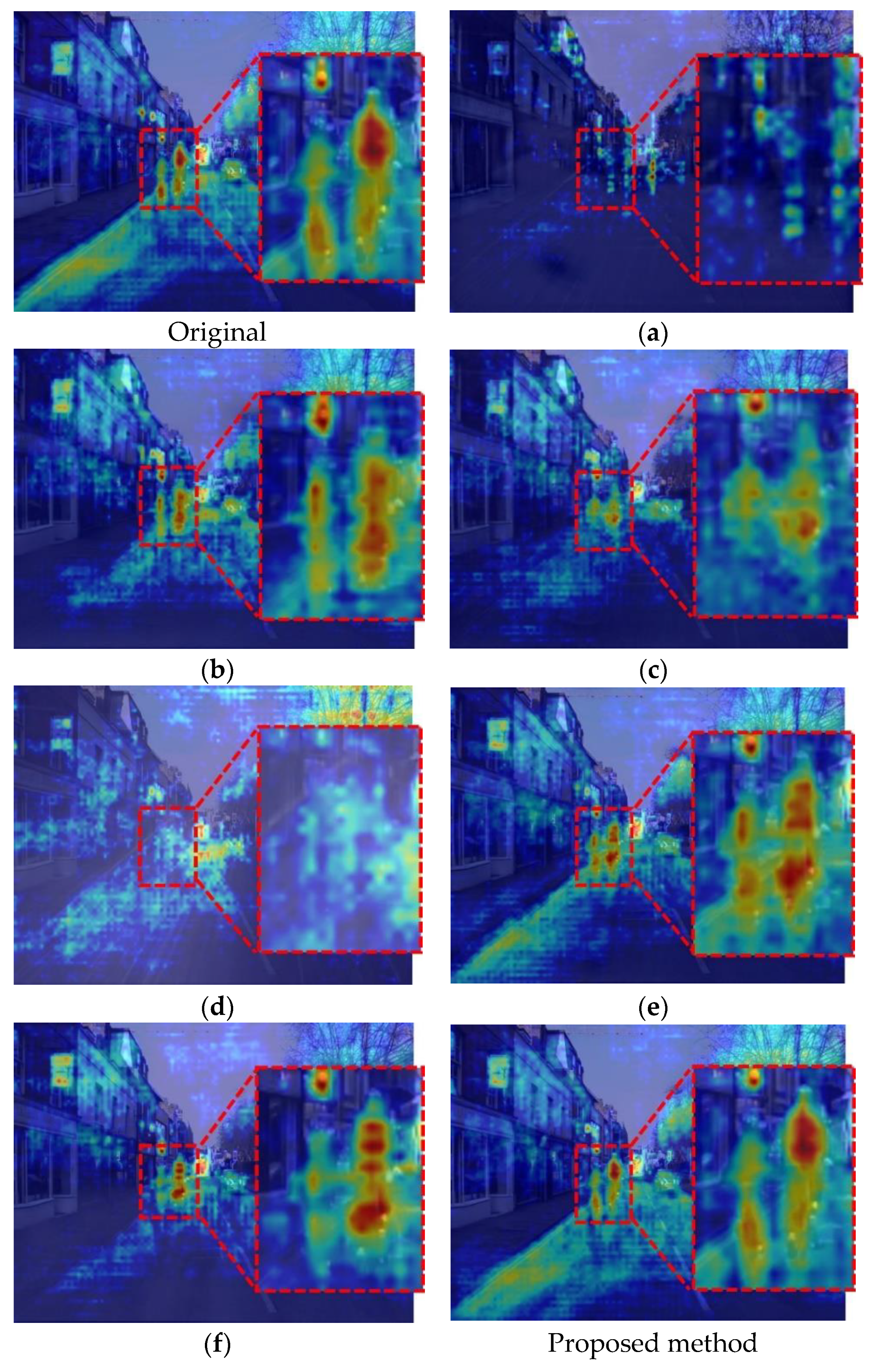
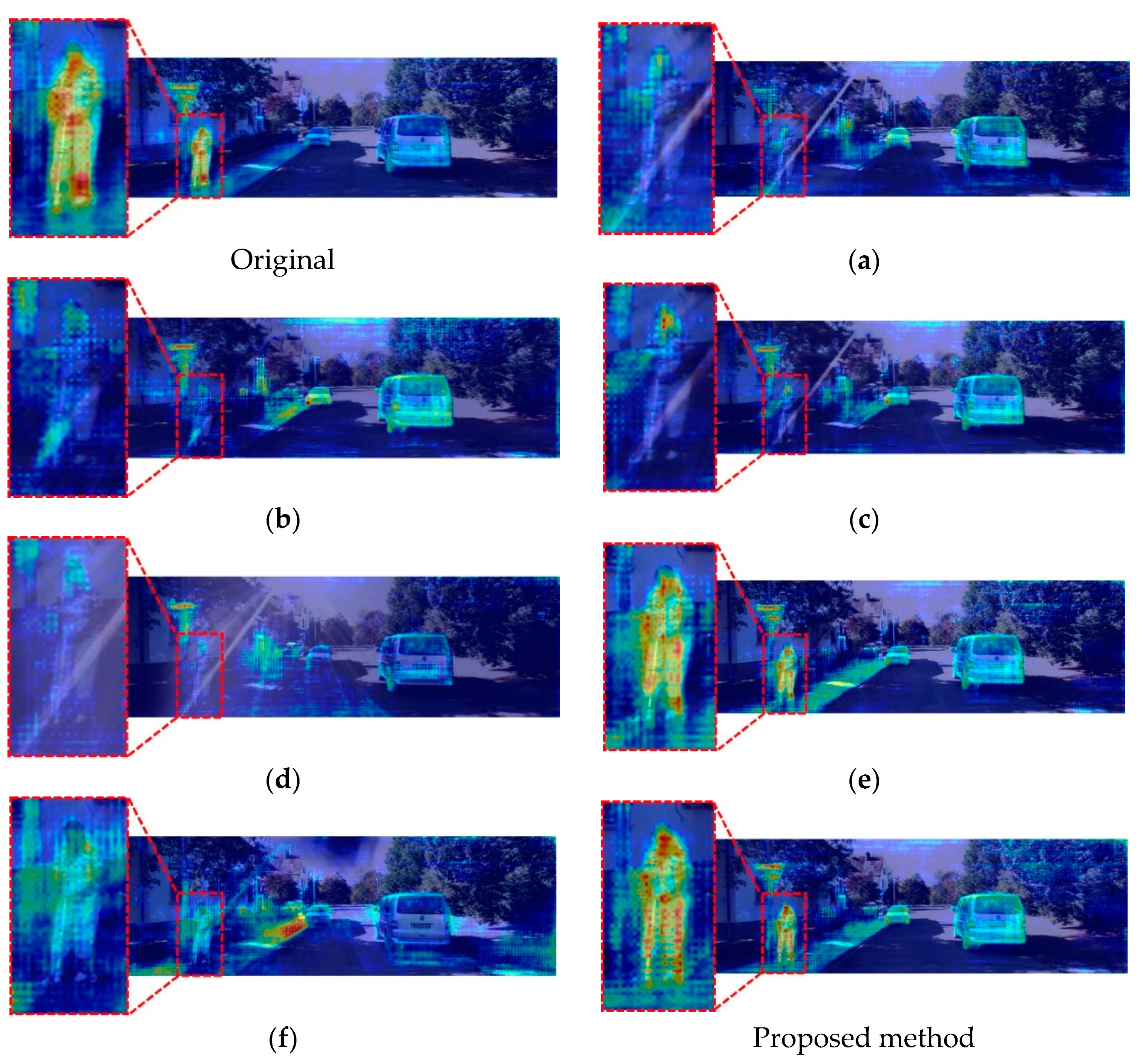
Figure 15 shows the results of extracting Grad-CAM for the bicyclist class when the original CamVid image was input in DeepLabV3+ [7], and when Grad-CAM [51] for the bicyclist class and the images restored by CAM-FRN and other methods were input in DeepLabV3+. And Figure 16 shows the results of extracting Grad-CAM for the pedestrian class when the original KITTI image is input in DeepLabV3+ [7], and when Grad-CAM [51] for the pedestrian class and the images restored by CAM-FRN and other methods are input in DeepLabV3+. After analyzing each figure, we found that our proposed method is the closest to the original image’s Grad-CAM.

Based on the analysis of the previous ablation study and comparative analysis with existing methods, we can provide the following reasons for the better performance of our proposed method compared with existing methods. Existing methods suffer from the problem of not removing artifacts properly when there are complex flare artifacts or there is a severe level of flare in the input image [9,21,22,23]. To solve these problems, we used CAM to provide additional information about the flare regions to the network, and reflected it in the loss function to successfully restore the parts covered by flare. Furthermore, we were able to consider composite flare artifacts. By doing so, we could achieve better restoration results compared with other methods, and based on the restoration results, we can see that the performance of our final goal, semantic segmentation, is also better than that of the existing restoration methods.

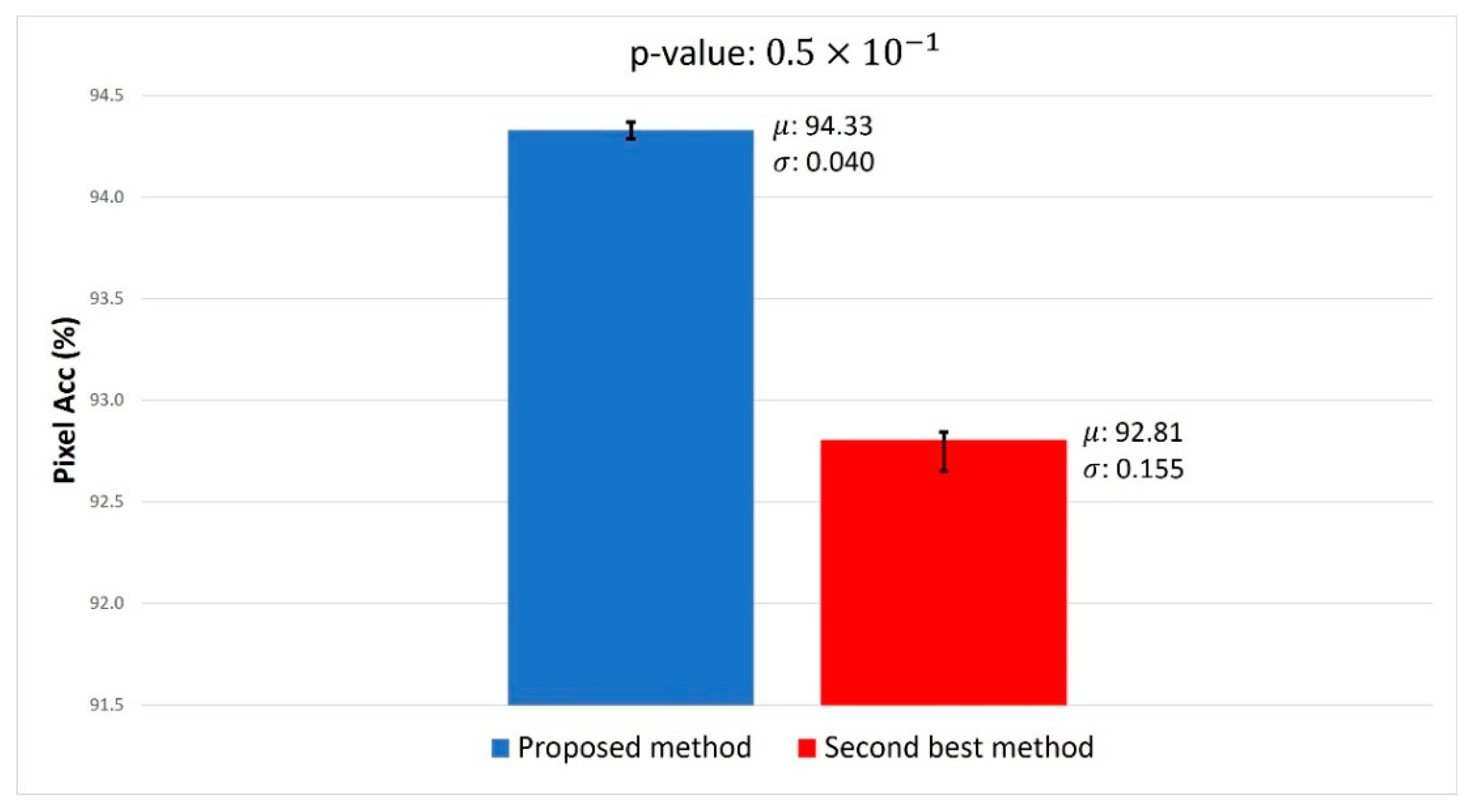
We calculate the p-values using the values of the proposed method and the second-best method among all semantic segmentation evaluation metrics in Table 24. We conducted t-test [52] and measured Cohen’s d-values [53] to demonstrate the significance of the performance difference between the two methods. As shown in Figure 17, the p-value of pixel accuracy is $0.5\times {10}^{-1}$, which indicates that a null hypothesis is rejected at the confidence interval of 95% and that the two methods have a difference in performance for pixel accuracy at the confidence interval of 95%. Subsequently, we measured Cohen’s d-value for pixel accuracy, and the result was 6.7363. The criteria for Cohen’s d-value are divided into 0.2, 0.5, and 0.8, which are distinguished into small, medium, and large effective sizes, respectively. Our Cohen’s d-value is greater than 0.8, which indicates that the performance difference between our method and the second-best method in terms of pixel accuracy is significantly large in the large effective size.

4.4. Computational Cost of Proposed Method

Lastly, we measured the parameters (Params), floating point operations (FLOPs), and multiply accumulate (MACs) to compare the computational costs of the proposed and previous methods. In

Table 28. Comparison of the measurement of parameters, MACs, and FLOPs between previous methods and the proposed method.

Method	Params (M)	MACs (G)	FLOPs (G)
Qiao et al. [23]	7.18	908.74	454.37
Wu et al. [9]	31.03	219.16	109.58
Pix2Pix [37]	54.40	725.85	362.93
CycleGAN [50]	6.07	227.46	113.73
FFANet [22]	44.56	1150.13	575.07
MPRNet [21]	36.37	1446.64	723.32
Proposed	39.46	773.95	386.98

, CycleGAN and Pix2Pix exhibited the lowest and highest number of parameters, respectively, while the proposed method exhibited the second highest number of parameters. In terms of MACs and FLOPs, [9] exhibited the lowest value while MPRNet had the highest value. The proposed method had the fourth highest value, thereby indicating that our method is heavy in terms of parameters but fourth most efficient in terms of computation amount. As shown in Table 14, Table 15, Table 16, Table 25, Table 26 and Table 27, excluding FFANet and MPRNet, which demonstrated the second and third best performance besides the proposed method, lens flare removal performance was poor for the syn-flare CamVid dataset and the syn-flare KITTI dataset, which also resulted in poor segmentation performance. In other words, the proposed method has the most efficient lens flare removal and semantic segmentation performance compared with other methods (FFANet, MPRNet, and proposed method).

5. Discussion

5.1. Limitations of Proposed Method

In this section, we analyze the failure cases of our proposed method when removing lens flare artifacts and related problems. The most serious problem is that not only the lens flare artifacts generated by the light source are removed, but also the light source is removed. A light source is an object that does not need to be removed because it is not an unnatural artifact. The problem occurs owing to the difficulty of finding datasets having images with lens flare and clean images without lens flare as input and label, respectively, and we must consider the semantic segmentation task for images captured by a frontal-viewing camera of a vehicle. It is challenging to find images that have a segmentation label while simultaneously considering a lens flare. Therefore, to solve the problem of insufficient data, we configured datasets by synthesizing lens flare artifacts into semantic segmentation datasets built by images captured using a frontal-viewing camera of a vehicle, such as CamVid [19] and KITTI [20]. Therefore, the target image being restored by removing a lens flare does not include a light source such as the sun, streetlight, and vehicle headlight, and the image generated by CAM-FRN is trained to remove a light source.

If Figure 18a,d,g,j become the input of CAM-FRN, the results shown in Figure 18c,f,i, are produced owing to a lack of information on a light source in Figure 18b,e,h,k, and the parts where a light source is located are placed with other pixel values. The model is trained to create images that are similar to the original images in Figure 18b,e,h,k, which is one of the problems to be resolved for lens flare removal. For removing lens flare artifacts more appropriately, further research is needed on finding methods to remove only the flare region by distinguishing a light source and the flare region.

Subsequently, we analyzed the cases of adequate and inadequate restoration of our proposed model. The first and second rows in Figure 19 show the cases where CAM-FRN inadequately removed lens flare in the syn-flare CamVid dataset. In both examples, lens flare generated on top of an object is removed, but the color of the original image is not restored compared with the ground-truth image. In the first row in Figure 19a, a traffic light is located close to a light source, and the intensity of a lens flare from the light source is fairly strong; therefore, the color of the traffic light shown in the original image (b) is not restored properly in the CAM-FRN result image in (c). In the second row in Figure 19d, the object is not located close to the light source as in the first case; however, a strong lens flare completely covers a person in the enlarged part. As a result, the color of a coat on the pedestrian in the original image (d) is not appropriately restored in the CAM-FRN result image in (f). In the third and last rows, the lens flare is effectively removed, and the color of an object covered by the flare is restored fairly adequately. Similar to (a) and (b), the object is covered by lens flare in (g) and (j) in the third and fourth rows, respectively; however, the pedestrians and the details of the building in the enlarged part are preserved adequately.

We analyzed the cases of successfully and unsuccessfully restoring the color details of an object behind a flare during adequate lens flare removal in the syn-flare KITTI dataset in Figure 20. In image (a) in the first row, lens flare is formed over a building, and the color of the building in the original image (b) is not properly restored in the CAM-FRN image (c) where the flare is removed. In image (b) in the second row, lens flare is formed over a building, and the paint color of the building in the original image (e) is not properly restored in the flare removal process and is shown as gray in image (f). Similar to the first and second rows, lens flare covers an object in images (g) and (j); however, lens flare is effectively removed, and the color of the object behind the flare is adequately preserved.

The cause of the result images in the first and second rows of Figure 19 and Figure 20 is the effect of lens flare on an image. Lens flare affects the contrast of an image, and a higher intensity of lens flare reduces the contrast. Therefore, lens flare in images (a) and (d) in Figure 19 and Figure 20 reduces their contrast, and the intensity of lens flare is high that the information of pixel values in the original image is severely lost. As the contrast value increases, dark areas become darker and bright areas become brighter, thereby creating a more evident contrast; however, the contrast between two areas becomes less in the opposite case. Because the contrast value is adjusted in proportion to the intensity of a pixel value, the loss of information of bright pixels before a lens flare increases as the contrast decreases. As a result, when lens flare is generated on objects with brighter pixel values, as shown in images (a) and (d) of Figure 19 and Figure 20, the pixel information in the original images (c) and (f) cannot be perfectly restored. However, in the third and fourth rows of Figure 19 and Figure 20, objects have relatively darker colors with low brightness or pixel intensity, and hence, lens flare is removed while retaining their colors to a certain extent. These limitations can adversely affect semantic segmentation, which is a pixel-wise classification task. Therefore, there is a need for research on methods for retaining the color and contrast of an image while removing lens flare.

5.2. Discussion of the Performance Analysis of the Proposed Method

As mentioned, we can see in Table 13 that the pixel accuracy metric is worse than the other results. However, we focused on the highest mIoU metric when utilizing all input images. Looking at Equation (33), pixel accuracy only considers true positives (TPs) and false positives (FPs). However, as we can see in Equation (35), mIoU additionally considers false negatives (FNs) and can also evaluate class misclassification, i.e., the possibility of class misclassification exists even if pixel accuracy is higher. Based on this rationale, we confirm that the proposed method utilizing all the inputs with the highest mIoU shows the best performance. In Table 16, we can see that our proposed method utilizing variational inference has a slightly worse SSIM score compared with the other results. However, we wanted to obtain an image with the most similar distribution of flare-free images and CAM-FRN outputs by using variational inference rather than simply considering the distance between pixels, as mentioned in the paper. The evaluation metric that can show this more clearly is the FID score, and we can see that the FID score is the best when using variational inference. We can also see in Table 17 that the proposed method using variational inference has the best segmentation performance. From this, we confirm that the FID score is more important than the other evaluation metrics in Table 16, and the best performance can be obtained when utilizing variational inference like the proposed method. In Table 26 and Table 27, “Original” means the segmentation accuracies using original images without flare, and they are the baseline accuracies. The important part of Table 26 and Table 27 is the performance over the segmentation network after flare removal, which can be seen in “With restoration use DeepLabV3+” in each table. We can see that the proposed method of “With restoration use DeepLabV3+” has the highest performance in each table. Table 28 compares the computational cost of the proposed method with previously studied methods. Although the proposed method does not show the best results compared with previous studies in Table 28, the segmentation accuracies by proposed method are higher than those by all the previous methods as shown in Table 24, Table 25, Table 26 and Table 27, and we focus on the segmentation accuracy rather than computational cost in our paper.

6. Conclusions

This study examined different methods for improving semantic segmentation performance by removing lens flares from images captured by frontal-viewing cameras in vehicles. This study is the first to solve the problem of an autonomous driving vehicle being unable to detect objects owing to a lens flare while simultaneously conducting lens flare removal and segmentation.

The proposed method removes a lens flare by extracting the lens flare region of an image as a class attention map and providing additional information on lens flare artifacts and lens flare region by creating additional inputs. Furthermore, we proposed ADCARB, which uses multi-scale feature learning and extracts the parts damaged by a lens flare as a mask for learning, which significantly improves the lens flare removal performance by using such a block. Additionally, we created an image that was as similar to the ground-truth image as possible through variational inference; self-attention was applied to the estimated latent space by executing variational inference to ensure global information was considered. The lens flare region mask obtained using CAM was reflected in style loss, content loss, adversarial loss, and discriminator loss, which improved the image quality by removing the lens flare with a focus on the flare region. When applying CAM-FRN to the segmentation task on the restored images, it demonstrated considerable performance improvements compared with previous restoration models [9,21,22], achieving a class accuracy of 67.34%, pixel accuracy of 94.33%, and mIoU of 71.26% on the syn-flare CamVid dataset. Additionally, CAM-FRN exhibited superior performance on the syn-flare KITTI dataset, attaining a class accuracy of 54.73%, pixel accuracy of 90.62%, and mIoU of 60.27%.

As mentioned in Section 5, CAM-FRN has the problem of removing flare artifacts while also removing light sources, and it has the problem of failing to restore the original color due to contrast being ruined by flare. In our follow-up research, we plan to design a restoration network that can accurately remove only lens flare by separating the light source and lens flare regions to address these issues. Furthermore, we plan to address the problem of being unable to restore color due to contrast being ruined properly. Our final goal is to work on an end-to-end network design that combines lens flare removal and semantic segmentation steps.

References

1. Badrinarayanan, V.; Kendall, A.; Cipolla, R. Segnet: A Deep Convolutional Encoder-Decoder Architecture for Image Segmentation. IEEE Trans. Pattern Anal. Mach. Intell. 2017, 39, 2481–2495. [Google Scholar] [CrossRef]
2. Zhao, H.; Shi, J.; Qi, X.; Wang, X.; Jia, J. Pyramid Scene Parsing Network. In Proceedings of the IEEE Conference on Computer Vision and Pattern Recognition, Honolulu, HI, USA, 21–26 July 2017; pp. 2881–2890. [Google Scholar]
3. Zhao, H.; Qi, X.; Shen, X.; Shi, J.; Jia, J. ICNet for Real-Time Semantic Segmentation on High-Resolution Images. In Proceedings of the ECCV 2018: 15th European Conference on Computer Vision (ECCV), Munich, Germany, 8–14 September 2018; pp. 405–420. [Google Scholar]
4. Chen, L.-C.; Papandreou, G.; Kokkinos, I.; Murphy, K.; Yuille, A.L. Semantic Image Segmentation with Deep Convolutional Nets and Fully Connected CRFs. arXiv 2014, arXiv:1412.7062. [Google Scholar]
5. Chen, L.-C.; Papandreou, G.; Kokkinos, I.; Murphy, K.; Yuille, A.L. Deeplab: Semantic Image Segmentation with Deep Convolutional Nets, Atrous Convolution, and Fully Connected CRFs. IEEE Trans. Pattern Anal. Mach. Intell. 2017, 40, 834–848. [Google Scholar] [CrossRef]
6. Chen, L.-C.; Papandreou, G.; Schroff, F.; Adam, H. Rethinking Atrous Convolution for Semantic Image Segmentation. arXiv 2017, arXiv:1706.05587. [Google Scholar]
7. Chen, L.-C.; Zhu, Y.; Papandreou, G.; Schroff, F.; Adam, H. Encoder-Decoder with Atrous Separable Convolution for Semantic Image Segmentation. In Proceedings of the ECCV 2018: 15th European Conference on Computer Vision (ECCV), Munich, Germany, 8–14 September 2018; pp. 801–818. [Google Scholar]
8. Ceccarelli, A.; Secci, F. RGB Cameras Failures and Their Effects in Autonomous Driving Applications. IEEE Trans. Dependable Secur. Comput. 2022, 20, 2731–2745. [Google Scholar] [CrossRef]
9. Wu, Y.; He, Q.; Xue, T.; Garg, R.; Chen, J.; Veeraraghavan, A.; Barron, J.T. How to Train Neural Networks for Flare Removal. In Proceedings of the IEEE/CVF International Conference on Computer Vision, Montreal, BC, Canada, 17 October 2021; pp. 2239–2247. [Google Scholar]
10. Zhang, Z.; Feng, H.; Xu, Z.; Li, Q.; Chen, Y. Single Image Veiling Glare Removal. J. Mod. Opt. 2018, 65, 2220–2230. [Google Scholar] [CrossRef]
11. Boynton, P.A.; Kelley, E.F. Liquid-Filled Camera for the Measurement of High-Contrast Images. In Proceedings of the Cockpit Displays X, Orlando, FL, USA, 21–25 April 2003; pp. 370–378. [Google Scholar]
12. Raskar, R.; Agrawal, A.; Wilson, C.A.; Veeraraghavan, A. Glare Aware Photography: 4D Ray Sampling for Reducing Glare Effects of Camera Lenses. In Proceedings of the SIGGRAPH ‘08: Special Interest Group on Computer Graphics and Interactive Techniques Conference, Los Angeles, CA, USA, 11–15 August 2008; pp. 1–10. [Google Scholar]
13. Talvala, E.-V.; Adams, A.; Horowitz, M.; Levoy, M. Veiling Glare in High Dynamic Range Imaging. ACM Trans. Graph. 2007, 26, 37-es. [Google Scholar] [CrossRef]
14. Wu, T.-P.; Tang, C.-K. A Bayesian Approach for Shadow Extraction from a Single Image. In Proceedings of the Tenth IEEE International Conference on Computer Vision (ICCV’05), Beijing, China, 17–21 October 2005; pp. 480–487. [Google Scholar]
15. Asha, C.S.; Bhat, S.K.; Nayak, D.; Bhat, C. Auto Removal of Bright Spot from Images Captured against Flashing Light Source. In Proceedings of the IEEE International Conference on Distributed Computing, VLSI, Electrical Circuits and Robotics (DISCOVER), Manipal, India, 11–12 August 2019; pp. 1–6. [Google Scholar]
16. Chabert, F. Automated Lens Flare Removal. In Technical Report; Department of Electrical Engineering, Stanford University: Stanford, CA, USA, 2015. [Google Scholar]
17. Vitoria, P.; Ballester, C. Automatic Flare Spot Artifact Detection and Removal in Photographs. J. Math. Imaging Vis. 2019, 61, 515–533. [Google Scholar] [CrossRef]
18. Koreban, F.; Schechner, Y.Y. Geometry by Deflaring. In Proceedings of the IEEE International Conference on Computational Photography (ICCP), San Francisco, CA, USA, 16–17 April 2009; pp. 1–8. [Google Scholar]
19. Brostow, G.J.; Fauqueur, J.; Cipolla, R. Semantic Object Classes in Video: A High-Definition Ground Truth Database. Pattern Recognit. Lett. 2009, 30, 88–97. [Google Scholar] [CrossRef]
20. Geiger, A.; Lenz, P.; Stiller, C.; Urtasun, R. Vision Meets Robotics: The Kitti Dataset. Int. J. Robot. Res. 2013, 32, 1231–1237. [Google Scholar] [CrossRef]
21. Zamir, S.W.; Arora, A.; Khan, S.; Hayat, M.; Khan, F.S.; Yang, M.-H.; Shao, L. Multi-Stage Progressive Image Restoration. In Proceedings of the IEEE Conference on Computer Vision and Pattern Recognition, CVPR 2021, Virtual. 19–25 June 2021; pp. 14821–14831. [Google Scholar]
22. Qin, X.; Wang, Z.; Bai, Y.; Xie, X.; Jia, H. FFA-Net: Feature Fusion Attention Network for Single Image Dehazing. In Proceedings of the AAAI Conference on Artificial Intelligence, New York, NY, USA, 7–14 February 2020; pp. 11908–11915. [Google Scholar]
23. Qiao, X.; Hancke, G.P.; Lau, R.W.H. Light Source Guided Single-Image Flare Removal from Unpaired Data. In Proceedings of the IEEE/CVF International Conference on Computer Vision, Montreal, BC, Canada, 11–17 October 2021; pp. 4157–4165. [Google Scholar]
24. Yu, F.; Koltun, V. Multi-Scale Context Aggregation by Dilated Convolutions. arXiv 2015, arXiv:1511.07122. [Google Scholar]
25. CAM-FRN. Available online: https://github.com/sunjong5108/CAM-based_Flare_Removal_Network (accessed on 10 January 2023).
26. Ronneberger, O.; Fischer, P.; Brox, T. U-Net: Convolutional Networks for Biomedical Image Segmentation. In Proceedings of the Medical Image Computing and Computer-Assisted Intervention (MICCAI), Munich, Germany, 5–9 October 2015; pp. 234–241. [Google Scholar]
27. Tu, Z.; Bai, X. Auto-Context and Its Application to High-Level Vision Tasks and 3d Brain Image Segmentation. IEEE Trans. Pattern Anal. Mach. Intell. 2009, 32, 1744–1757. [Google Scholar]
28. Kontschieder, P.; Bulo, S.R.; Bischof, H.; Pelillo, M. Structured Class-Labels in Random Forests for Semantic Image Labelling. In Proceedings of the IEEE International Conference on Computer Vision, ICCV 2011, Barcelona, Spain, 6–13 November 2011; pp. 2190–2197. [Google Scholar]
29. Gonfaus, J.M.; Boix, X.; Van de Weijer, J.; Bagdanov, A.D.; Serrat, J.; Gonzalez, J. Harmony Potentials for Joint Classification and Segmentation. In Proceedings of the 2010 IEEE Computer Society Conference on Computer Vision and Pattern Recognition, San Francisco, CA, USA, 13–18 June 2010; pp. 3280–3287. [Google Scholar]
30. Kohli, P.; Torr, P.H. Robust Higher Order Potentials for Enforcing Label Consistency. Int. J. Comput. Vis. 2009, 82, 302–324. [Google Scholar] [CrossRef]
31. Zhang, C.; Wang, L.; Yang, R. Semantic Segmentation of Urban Scenes Using Dense Depth Maps. In Proceedings of the 11th European Conference on Computer Vision, Heraklion, Crete, Greece, 5–11 September 2010; pp. 708–721. [Google Scholar]
32. He, K.; Zhang, X.; Ren, S.; Sun, J. Deep Residual Learning for Image Recognition. In Proceedings of the IEEE Computer Society Conference on Computer Vision and Pattern Recognition (CVPR), Las Vegas, NV, USA, 27–30 June 2016; pp. 770–778. [Google Scholar] [CrossRef]
33. Ahn, J.; Cho, S.; Kwak, S. Weakly Supervised Learning of Instance Segmentation With Inter-Pixel Relations. In Proceedings of the IEEE/CVF Conference on Computer Vision and Pattern Recognition, Long Beach, CA, USA, 15–20 June 2019; pp. 2204–2213. [Google Scholar]
34. Kingma, D.; Welling, M. Auto-Encoding Variational Bayes. arXiv 2014, arXiv:1312.6114. [Google Scholar]
35. Doersch, C. Tutorial on Variational Autoencoders. arXiv 2021, arXiv:1606.05908. [Google Scholar]
36. Im, D.J.; Ahn, S.; Memisevic, R.; Bengio, Y. Denoising Criterion for Variational Auto-Encoding Framework. In Proceedings of the Thirty-First AAAI Conference on Artificial Intelligence (AAAI-17), San Francisco, CA, USA, 31 February 2017; pp. 2059–2065. [Google Scholar]
37. Isola, P.; Zhu, J.-Y.; Zhou, T.; Efros, A.A. Image-to-Image Translation with Conditional Adversarial Networks. In Proceedings of the IEEE Conference on Computer Vision and Pattern Recognition, Honolulu, HI, USA, 21–26 July 2017; pp. 1125–1134. [Google Scholar]
38. Hendrycks, D.; Gimpel, K. Gaussian Error Linear Units (GELUs). arXiv 2020, arXiv:1606.08415. [Google Scholar]
39. Agarap, A.F. Deep Learning Using Rectified Linear Units (ReLU). arXiv 2018, arXiv:1803.08375. [Google Scholar]
40. Zeng, Y.; Fu, J.; Chao, H.; Guo, B. Aggregated Contextual Transformations for High-Resolution Image Inpainting. IEEE Trans. Vis. Comput. Graph. 2022, 29, 3266–3280. [Google Scholar] [CrossRef]
41. Ramachandran, P.; Parmar, N.; Vaswani, A.; Bello, I.; Levskaya, A.; Shlens, J. Stand-Alone Self-Attention in Vision Models. In Proceedings of the Advances in Neural Information Processing Systems 32 (NeurIPS 2019), Vancouver, BC, Canada, 8–14 December 2019; pp. 1–13. [Google Scholar]
42. Gatys, L.A.; Ecker, A.S.; Bethge, M. Image Style Transfer Using Convolutional Neural Networks. In Proceedings of the IEEE Conference on Computer Vision and Pattern Recognition, Las Vegas, NV, USA, 27–30 June 2016; pp. 2414–2423. [Google Scholar]
43. Simonyan, K.; Zisserman, A. Very Deep Convolutional Networks for Large-Scale Image Recognition. arXiv 2014, arXiv:1409.1556. [Google Scholar]
44. Wu, T.; Tang, S.; Zhang, R.; Cao, J.; Zhang, Y. CGNet: A Light-Weight Context Guided Network for Semantic Segmentation. IEEE Trans. Image Process. 2021, 30, 1169–1179. [Google Scholar] [CrossRef]
45. NVIDIA GeForce RTX 3090. Available online: https://www.nvidia.com/en-us/geforce/graphics-cards/30-series/rtx-3090-3090ti/ (accessed on 3 June 2022).
46. PyTorch. Available online: https://pytorch.org/ (accessed on 3 June 2022).
47. K-Fold Cross-Validation. Available online: https://en.wikipedia.org/wiki/Cross-validation_(statistics) (accessed on 11 August 2020).
48. Kingma, D.P.; Ba, J. Adam: A method for stochastic optimization. arXiv 2014, arXiv:1412.6980. [Google Scholar]
49. Szegedy, C.; Vanhoucke, V.; Ioffe, S.; Shlens, J.; Wojna, Z. Rethinking the Inception Architecture for Computer Vision. In Proceedings of the 2016 IEEE Conference on Computer Vision and Pattern Recognition (CVPR), Las Vegas, NV, USA, 27–30 June 2016; pp. 2818–2826. [Google Scholar]
50. Zhu, J.-Y.; Park, T.; Isola, P.; Efros, A. Unpaired Image-to-Image Translation Using Cycle-Consistent Adversarial Networks. In Proceedings of the 2017 IEEE International Conference on Computer Vision (ICCV), Venice, Italy, 22–29 October 2017; pp. 2223–2232. [Google Scholar]
51. Selvaraju, R.R.; Cogswell, M.; Das, A.; Vedantam, R.; Parikh, D.; Batra, D. Grad-CAM: Visual Explanations From Deep Networks via Gradient-Based Localization. In Proceedings of the 2017 IEEE International Conference on Computer Vision ICCV, Venice, Italy, 22–29 October 2017; pp. 618–626. [Google Scholar]
52. Student’s T-Test. Available online: https://en.wikipedia.org/wiki/Student%27s_t-test (accessed on 3 September 2020).
53. Cohen, J. A Power Primer. In Methodological Issues and Strategies in Clinical Research, 4th ed; American Psychological Association: Washington, DC, USA, 2016; p. 284. ISBN 978-1-4338-2091-5. [Google Scholar]
Figure 1. Process of lens flare artifacts being generated inside a camera.
Mathematics 11 03644 g001
Figure 2. The effect of a lens flare on the results of semantic segmentation. (a) Original image before synthesizing a lens flare, (b) segmentation ground-truth label, (c) semantic segmentation result by DeepLabV3+ of (a), (d) image after synthesizing a lens flare, and (e) semantic segmentation result by DeepLabV3+ of (d).
Mathematics 11 03644 g002
Figure 3. Overall procedure of the proposed method.
Mathematics 11 03644 g003
Figure 4. (a) Input image including lens flare artifacts, (b) CAM of (a), (c) multiplication of (a,b), (d) binary mask wherein the flare region created by (b) has a value of 1 and the remaining regions have value 0, and (e) mask covering the flare region created by using (d).
Mathematics 11 03644 g004
Figure 5. CAM-FRN architecture.
Mathematics 11 03644 g005
Figure 6. ADCARB structure.
Mathematics 11 03644 g006
Figure 7. Self-attention module in the proposed method.
Mathematics 11 03644 g007
Figure 8. DeepLabV3 + architecture.
Mathematics 11 03644 g008
Figure 9. Original images of CamVid and KITTI datasets, and the images synthesized with lens flare artifacts. (a,c) Original images of the CamVid and KITTI datasets, and (b,d) images with lens flare artifacts synthesized with (a,c).
Mathematics 11 03644 g009
Figure 10. Generator and discriminator loss graphs of the syn-flare CamVid dataset.
Mathematics 11 03644 g010
Figure 11. Comparison of the restoration results of the proposed method and state-of-the-art methods for the syn-flare CamVid dataset. (a) Restoration result of the method proposed by Qiao et al.; (b) restoration result of the method proposed by Wu et al.; (c) restoration result of Pix2Pix, one of image-to-image translation methods; (d) restoration result of CycleGAN; (e) restoration result of FFANet proposed for dehazing; and (f) restoration result of MPRNet proposed for deraining. The last image is the lens flare removal result of our proposed method.
Mathematics 11 03644 g011
Figure 12. This figure compares the restoration results of the proposed method and state-of-the-art methods for the syn-flare KITTI dataset: (a) restoration result of the method proposed by Qiao et al.; (b) restoration result of the method proposed by Wu et al.; (c) restoration result of Pix2Pix, one of image-to-image translation methods; (d) restoration result of CycleGAN; (e) restoration result of FFANet proposed for dehazing; and (f) restoration result of MPRNet proposed for deraining. The last image is the lens flare removal result of our proposed method.
Mathematics 11 03644 g012
Figure 13. Semantic segmentation test results of the image restored by the proposed method and state-of-the-art methods for the syn-flare CamVid dataset. (a) Segmentation result of the image restored by the method of Qiao et al.; (b) segmentation result of the image restored by the method of Wu et al.; (c) segmentation result of the image restored by Pix2Pix, one of image-to-image translation methods; (d) segmentation result of the image restored by CycleGAN; (e) segmentation result of the image restored by FFANet proposed for dehazing; and (f) the segmentation result of the image restored by MPRNet proposed for deraining. The last image shows the segmentation result of the image from which a lens flare is removed by our proposed method.
Mathematics 11 03644 g013
Figure 14. This figure shows the semantic segmentation test results of the images restored by the proposed method and state-of-the-art methods for the syn-flare KITTI dataset: (a) segmentation result of the image restored by the method of Qiao et al.; (b) segmentation result of the image restored by the method of Wu et al.; (c) segmentation result of the image restored by Pix2Pix, one of image-to-image translation methods; (d) segmentation result of the image restored by CycleGAN; (e) segmentation result of the image restored by FFANet proposed for dehazing; and (f) segmentation result of the image restored by MPRNet proposed for deraining. The last image shows the segmentation result of the image from which a lens flare is removed by our proposed method.
Mathematics 11 03644 g014
Figure 15. Grad-CAM for the bicyclist class when segmentation is performed using the restoration results according to the input combination in the syn-flare CamVid dataset: (a) the method of Qiao et al.; (b) the method of Wu et al.; (c) Pix2Pix which is one of image-to-image translation methods; (d) CycleGAN; (e) FFANet which is proposed for dehazing; and (f) MPRNet which is proposed for deraining. The last image is the case of our proposed method.
Mathematics 11 03644 g015
Figure 16. This figure shows the Grad-CAM for the pedestrian class when segmentation is performed using the restoration results according to the input combination in the syn-flare KITTI dataset: (a) the method of Qiao et al.; (b) the method of Wu et al.; (c) Pix2Pix which is one of image-to-image translation methods; (d) CycleGAN; (e) FFANet which is proposed for dehazing; and (f) MPRNet which is proposed for deraining. The last image is the case of our proposed method.
Mathematics 11 03644 g016
Figure 17. t-test results of our proposed method’s pixel accuracy and the second-best method (FFANet + DeepLabV3+)’s pixel accuracy in the syn-flare CamVid dataset.
Mathematics 11 03644 g017
Figure 18. Failure cases of CAM-FRN in each dataset. In the syn-flare CamVid dataset, (a,d) are the input image of each row, (b,e) are the ground-truth image of each row, and (c,f) are the prediction image of CAM-FRN of each row. In the syn-flare KITTI dataset, (g,j) are the input image of each row, (h,k) are the ground-truth image of each row, and (i,l) are the prediction image of CAM-FRN of each row.
Mathematics 11 03644 g018
Figure 19. Successful and unsuccessful restoration cases of CAM-FRN in the syn-flare CamVid dataset. Images of unsuccessful restoration: (a,d) input images, (b,e) ground-truth images, and (c,f) prediction images. Images of successful restoration: (g,j) input images, (h,k) ground-truth images, and (i,l) prediction images.
Mathematics 11 03644 g019
Figure 20. Successful and unsuccessful restoration cases of CAM-FRN in the syn-flare KITTI dataset. Images of unsuccessful restoration: (a,d) input images, (b,e) ground-truth images, and (c,f) prediction images. Images of successful restoration: (g,j) input images, (h,k) ground-truth images, and (i,l) prediction images.
Mathematics 11 03644 g020