A Mathematical Solution to the Computational Fluid Dynamics (CFD) Dilemma

Abstract

Turbulent flows of practical relevance are often characterized by high Reynolds numbers and solid boundaries. The need to account for flow separation seen in such flows requires the use of (partially) resolving simulation methods on relatively coarse grids. The development of such computational methods is characterized by stagnation. Basically, only a few methods are regularly applied that are known to suffer from significant shortcomings: such methods are often characterized by the significant uncertainty of the predictions due to a variety of adjustable simulation settings, their computational cost can be essential because performance shortcomings need to be compensated by a higher resolution, and there are questions about their reliability because the flow resolving ability is unclear; hence, all such predictions require justification. A substantial reason for this dilemma is of a conceptual nature: the lack of clarity about the essential questions. The paper contrasts the usually applied simulation methods with the minimal error simulation methods presented recently. The comparisons are used to address essential questions about the required characteristics of the desired simulation methods. The advantages of novel simulation methods (including their simplicity, significant computational cost reductions, and controlled resolution ability) are pointed out.

1. Introduction

Computational fluid dynamics (CFD) focuses on the analysis and prediction of fluid flow based on the numerical solution of fluid flow conservation equations. It has impacted and transformed all aspects of human endeavor and industry. CFD essentially matters to aerospace, defense, energy, power generation, transport, electronics, food processing, environmental management, fire safety, computational chemistry, particle physics, genetics, architecture and building design, and life, biomedical, and pharmaceutical sciences [1]. An indication of how many people are involved in CFD is given by the about 25,000 OpenFOAM users in 2022 [2] (OpenFOAM is open source CFD software used by a part of the community). According to the CFD company ANSYS, ANSYS is used by 21,251 companies with 50–200 employees and USD 1M-10M in revenue [3]. The global CFD (both commercial and inhouse research and development by government and private industry) is today approximately worth tens of billions USD and is growing at a fast pace [1].

There are significant challenges for CFD in regard to the solution to problems of practical relevance. The latter are usually characterized by a very high Reynolds number ($Re$) and complex geometries. A very important characteristic feature of such flows is the appearance of a separated flow. A typical illustration of separated turbulent flows is given in Figure 1. This figure shows the velocity streamlines in periodic hill flows (channel flow with embedded hills at the lower wall on the left-hand side (LHS) and right-hand side (RHS), and there is flow from the left to the right). This flow involves features such as separation, recirculation, and natural reattachment [4,5,6,7,8]. In particular, the bubble in Figure 1 next to the hill on the LHS characterizes a reversed flow region (separated flow). Such flow separation is highly relevant to a large variety of industrial applications, see e.g., ref. [9]. A specific illustration of aerospace grand challenge problems is given in Figure 2.

Unfortunately, direct numerical simulation (DNS) is inapplicable to most problems of practical relevance because of its extreme computational cost for high $Re$ turbulent flow simulations [11], and the usually applied methods like the Reynolds-averaged Navier–Stokes (RANS), large eddy simulation (LES), and hybrid RANS-LES methods provide an inappropriate basis to properly address the challenges described in Figure 2. These methods suffer from the well-known problems characterized in

Table 1. The CFD dilemma: unsolved problems of the RANS, hybrid RANS-LES (the WMLES and DES), and the LES. See also Section 3.3 regarding the mismatch of the imposed and actual resolution.

increasing cost, uncertainty remains	↑	Method	Typical problems requiring validation of all such simulation results
		LES	artificial length scale $\Delta$ in model viscosity ${\nu }_t=C_{\mu }{k}^{1/2}\Delta$ implies uncertain resolution or high cost to ensure a proper resolution via a sufficiently small $\Delta$
		RANS-LES: WMLES/DES	significant uncertainty depending on a variety of simulation settings and high cost required to compensate the mismatch of imposed and actual resolution
		RANS	unreliable (can be very inaccurate) and the exclusion of instantaneous turbulence implies unphysical simulations of separated turbulent flows

(WMLES and DES refer to wall-modeled LES and detached eddy simulation, respectively). The resulting CFD dilemma is a significant waste of resources. In particular, all such existing methods require validation of their results, which is often hardly possible because experimental data are hardly available for very high $Re$ flows seen in reality. It is worth noting that corresponding issues do not only apply to the problems indicated in Figure 2 but to a variety of other problems, as, for example, mesoscale and microscale modeling in regard to atmospheric simulations and many technical applications [12,13,14,15].

The motivation for this paper is to explain the need for the improvement of the usually applied simulation methods for turbulent flows and ways to overcome such significant issues. The problems and their relevance are specified in Section 2. Novel simulation methods based on exact mathematics and their implications for the usually applied methods are presented in Section 3. Conclusions are presented in Section 4.

2. The CFD Dilemma

2.1. The RANS, LES, and Hybrid RANS-LES Methods

The success of CFD is based on equations that are solved numerically. Let us summarize first the basic concepts to illustrate the current development of CFD equation methods.

We consider an incompressible flow for simplicity, the extension to a compressible flow (possibly involving scalar transport) is straightforward; see ref. [16]. The common mathematical basis for the RANS, LES, and hybrid RANS-LES models is given by the incompressible continuity equation $\partial {\tilde{U}}_i/\partial x_i=0$ and the momentum equation

$$\frac{D{\tilde{U}}_i}{Dt}=-\frac{\partial (\tilde{p}/\rho +2k/3)}{\partial x_i}+2\frac{\partial (\nu +{\nu }_t){\tilde{S}}_{ik}}{\partial x_k}.$$

(1)

Here, $D/Dt=\partial /\partial t+{\tilde{U}}_k\partial /\partial x_k$ denotes the filtered Lagrangian time derivative, and the sum convention is used throughout this paper. ${\tilde{U}}_i$ refers to the $i^{th}$ component of the spatially filtered velocity. We have here the filtered pressure $\tilde{p}$, $\rho$ is the constant mass density, k is the modeled energy, $\nu$ is the constant kinematic viscosity, and ${\tilde{S}}_{ij}=(\partial {\tilde{U}}_i/\partial x_j+\partial {\tilde{U}}_j/\partial x_i)/2$ is the rate-of-strain tensor. Usually, the modeled viscosity is given by ${\nu }_t=C_{\mu }{k}^{1/2}L$. Here, $C_{\mu }$ is a model parameter with standard value $C_{\mu }=0.09$, and L is a characteristic length scale. The latter can be related to the dissipation rate $ϵ=k/\tau$ of the modeled kinetic energy, the dissipation time scale $\tau$, or the turbulence frequency $\omega =1/\tau$ by $L=k^{3/2}/ϵ=k^{1/2}\tau =k^{1/2}/\omega$, respectively. The RANS and LES approaches differ by different settings of the characteristic length scales L in ${\nu }_t=C_{\mu }{k}^{1/2}L$ and the different grids applied.

The RANS applies transport equations for k and, for example, the dissipation $ϵ$,

$$\frac{Dk}{Dt}=P-ϵ+D_k,\frac{Dϵ}{Dt}=C_{{ϵ}_1}\frac{{ϵ}^2}{k}\left(\frac{P}{ϵ}-\alpha \right)+D_{ϵ},$$

(2)

which determine L via $L=k^{3/2}/ϵ$. The diffusion terms are given by $D_k=\partial [{\nu }_t\partial k/\partial x_j]/\partial x_j$, $D_{ϵ}=\partial [({\nu }_t/{\sigma }_{ϵ})\partial ϵ/\partial x_j]/\partial x_j$, and $P={\nu }_t{S}^2$ is the production of k, where $S={\left(2{\tilde{S}}_{mn}{\tilde{S}}_{nm}\right)}^{1/2}$ is the characteristic shear rate. $C_{{ϵ}_1}$ is a constant with standard value $C_{{ϵ}_1}=1.44$, ${\sigma }_{ϵ}=1.3$, and $\alpha =C_{{ϵ}_2}/C_{{ϵ}_1}$, where $C_{{ϵ}_2}=1.92$ [17] implies $\alpha =1.33$. In contrast to the RANS approach focusing on the modeling of characteristic turbulence length scales, the LES applies a length scale that is supposed to be small compared to the RANS length scale. The usual setting is $L=\Delta$. Here, $\Delta$ refers to the filter width, which is proportional to the grid. Sometimes, minor variations of $L=\Delta$ are considered (see ref. [18], Section 2.3). The latter are not considered here for simplicity.

The different L settings applied in the RANS (LES) in conjunction with coarse (fine) computational grids have remarkable consequences, which are illustrated in Figure 3: the LES (RANS) concept is shown on the LHS (RHS). Due to the relatively large modeled viscosity, turbulent velocity fluctuations are not resolved in the RANS on coarse grids. All the turbulent motion is modeled, and we talk about modeled motion. In contrast, due to the relatively small modeled viscosity, turbulent velocity fluctuations are resolved in the LES on sufficiently fine grids. This means the LES involves two simulation ingredients: modeled motion represented by the equations applied and resolved motion represented by the resolved velocity fluctuations. Correspondingly, the RANS and LES simulation concepts show remarkable differences in simulations. The RANS methods are computationally very efficient because they run in steady mode, and coarse grids can be applied. However, in regard to separated turbulent flows (see the illustration in Figure 1), which are usually seen in applications involving solid boundaries, the RANS were found to provide unreliable turbulent flow predictions because of their inability to properly reflect instantaneous turbulence. There is a substantial amount of work aiming at the improvement of RANS predictions for separated flow by the involvement of machine learning methods. However, so far there is no convincing demonstration that such methods can overcome the typical RANS issues, see ref. [19]. The LES usually provides much more reliable predictions because of the ability to involve instantaneous flow. However, the need to apply a sufficiently fine computational grid makes the LES very often unaffordable for simulations of complex high-$Re$ flows seen in reality: see Section 2.3.

The only promising approach to deal with this problem is an appropriate hybridization of the RANS and LES [9,18,20,21]. A variety of approaches for combining the RANS and LES equations have been suggested so far, for example, the wall-modeled LES (WM-LES) [22,23,24,25,26], the detached eddy simulation (DES) applied in conjunction with several equations [21,27,28,29,30,31,32], the Reynolds-stress-constrained LES (RSC-LES) [33], unified RANS-LES (UNI-LES) [34,35,36,37,38,39,40,41,42,43,44,45,46,47], the partially averaged Navier–Stokes (PANS) [48], the partially integrated transport modeling (PITM) [49,50], and the scale adaptive simulation (SAS) methods [21,51,52]. Figure 4 illustrates the use of hybrid RANS-LES methods. The data shown on the LHS were obtained by searching in ScienceDirect for journal papers and books that referred to the mentioned phrase in the title, abstract, or keywords. More specifically, the record of blending methods was obtained by searching for “blending turbulence model”. A corresponding search for unsteady RANS (URANS) (not shown) provided a trend almost equivalent to the DES trend. The plot on the RHS of Figure 4 refers to papers that addressed typical problems of popular CFD methods: “log-layer mismatch”, “grid-induced separation”, or “hybrid gray area”. Interesting observations related to Figure 4 are as follows. First, there is a large variety of hybrid RANS-LES methods, but only a few methods are regularly applied, first of all, the WMLES and DES methods and then three other methods. Both the WMLES and DES are known to suffer from significant shortcomings. Second, the cumulative number of papers that addressed modeling issues shows that there is a very limited number of attempts (a total of 15 papers according to this search, which may give only a partial impression) to address the typical modeling issues of popular hybrid RANS-LES methods. Correspondingly, the predominant opinion of the community in this regard is “There exist two kinds of LES-RANS hybrid methodology: one is WMLES and the other being detached-eddy simulation (DES)” [53].

2.2. The CFD Dilemma

Due to the computational cost and simulation performance, the general CFD dilemma is that resolving simulations on relatively coarse grids are required, but the currently applied concepts do not provide a proper basis for that (see the overview in Table 1). This is described now explicitly by focusing on the DES and WMLES because of the reasons pointed out in the preceding paragraph. In particular, the next two paragraphs focus on the WMLES, the following two paragraphs focus on the DES, and the last paragraph focuses on the LES.

The main thrust of the WMLES is on providing appropriate boundary conditions for the LES performed on relatively coarse grids by using a RANS model close to the wall. The latter can be accomplished, e.g., by a simplified version of the momentum Equation (1) used to solve for the wall shear stress,

$$2\frac{\partial (\nu +{\nu }_t){\tilde{S}}_{i2}}{\partial x_2}=\frac{D{\tilde{U}}_i}{Dt}+\frac{\partial (\tilde{p}/\rho +2k/3)}{\partial x_i}=F_i.$$

(3)

The abbreviation $F_i$ is used to refer to the previous expression. The modeled viscosity ${\nu }_t$ represents the difference between the total and resolved contributions, ${\nu }_t={\nu }_{t,tot}-{\nu }_{t,res}$. Usually, the resolved contribution ${\nu }_{t,res}$ is neglected, which may imply significant errors. Thus, Park and Moin [54] suggested applying ${\nu }_t={\nu }_{t,tot}-{\nu }_{t,res}$ in conjunction with a prescribed RANS viscosity given by ${\nu }_{t,tot}$. In this approach, the RANS is applied only to a thin layer near the wall, where the layer thickness may be much smaller than the boundary layer thickness. This method captures most of the turbulence inside the boundary layer by the LES without resolving the smallest scales above the viscous sublayer [53].

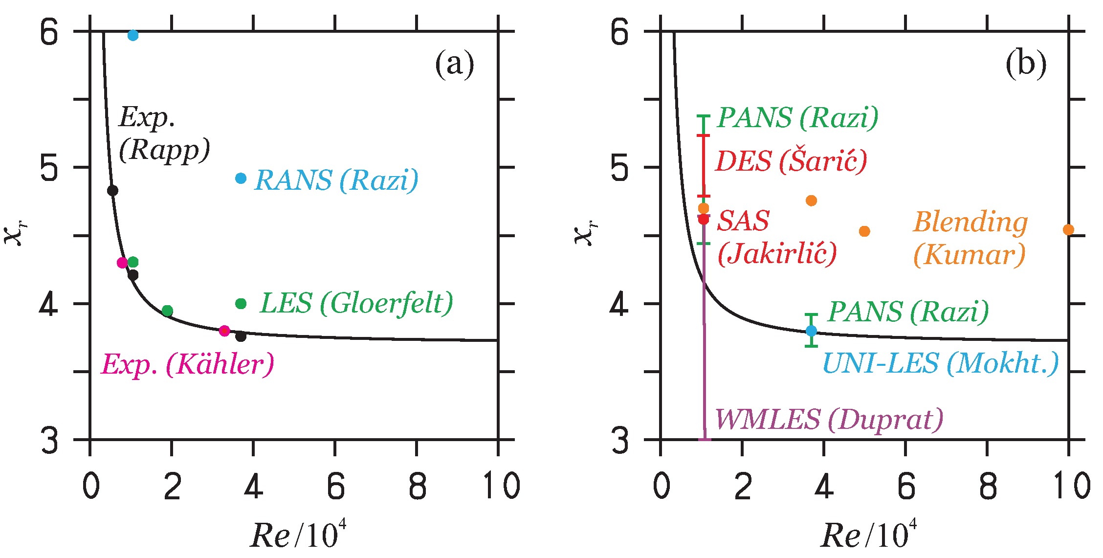
However, the concept of the WMLES faces issues. An adequate resolution of the boundary layer thickness (which makes the WMLES orders of magnitude more expensive than the original DES [25]) as expected is not feasible under many conditions, e.g., in thin laminar boundary layers. The off-wall location, where the LES is coupled to the wall model, needs to be prescribed as a fraction of the local boundary layer thickness, but the boundary layer thickness is unknown a priori for complex geometries [25,26]. Different computational mesh distributions can significantly affect the WMLES results for the same number of grid points [55]. An illustration of the uncertainty of the WMLES predictions in comparison to experiments, the RANS, LES, and other hybrid RANS-LES is given in Figure 5 regarding periodic hill flows: the corresponding reattachment point (see Figure 1, the point at about $x/h=3.8$) predictions obtained by different methods are shown for a range of $Re$. We see large prediction uncertainties depending on the simulation settings.

The basic DES concept, which can be applied in a variety of turbulence equations, is a switch of the LES and RANS length scales. The following equation can be used, for example,

$$\frac{Dk}{Dt}=P-\psi ϵ+D_k,\frac{Dϵ}{Dt}=C_{{ϵ}_1}\frac{{ϵ}^2}{k}\left(\frac{P}{ϵ}-\alpha \right)+D_{ϵ}.$$

(4)

Here, a function $\psi =max(1,L/[C_{DES}\Delta ])$ is involved, where $C_{DES}$ is a proportionality coefficient. An alternative writing of the dissipation $\psi ϵ$ in the k equation is $\psi ϵ=k^{3/2}/L_{DES}$, where the DES length scale $L_{DES}=min(L,C_{DES}\Delta )$ is used. The DES treats a major part of the attached boundary layer by the RANS, and the LES is applied in separated flow regions [66, 76]. A typical problem of the original DES is grid-induced separation, triggered by the shifting from the RANS to the LES. This problem can be addressed by a delayed DES (DDES), which prevents the shifting from the RANS to the LES within the boundary layer. Within this approach [28], $L_{DES}$ is replaced by $L_{DDES}=L-fmax(0,L-C_{DES}\Delta )$, which involves $f=1-tanh\left[{\left(20\eta \right)}^3\right]$. Here, $\eta =(\nu +{\nu }_t)/\left({\kappa }^2{L}^2{[\partial {\tilde{U}}_i/\partial x_j\partial {\tilde{U}}_i/\partial x_j]}^{1/2}\right)$, with $\kappa$ being the von Kármán constant. There is also the improved delayed DES (IDDES), which uses a blending of the DDES and the WMLES to enable the WMLES near the wall [29]. However, such improvements are no guarantee of a better model performance in simulations [45].

The basic problem of the DES concepts is the idea that a desired flow resolution in between the RANS and LES can be imposed by the model. A specific discussion of this problem is provided in Section 3.3 after presenting different simulation methods. The core conclusion can be illustrated by considering the PANS and PITM concepts instead of the DES concept. The PANS and PITM concepts apply a hybridization of the dissipation term in the scale equation instead of the dissipation in the k equation,

$$\frac{Dk}{Dt}=P-ϵ+D_k,\frac{Dϵ}{Dt}=C_{{ϵ}_1}\frac{{ϵ}^2}{k}\left(\frac{P}{ϵ}-{\alpha }_P\right)+D_{ϵ},$$

(5)

where ${\alpha }_P=1+R(\alpha -1)$. The equivalence of such modifications of different dissipation terms is well known [10,62,63,64]. The R involved in ${\alpha }_P=1+R(\alpha -1)$ represents the resolution degree (equivalent to $L_{+}^2$, see Equation (13) below). In the PANS, this resolution degree is imposed, and it is provided by a constant. In the PITM, the resolution degree is also imposed; $R=1.06{\Delta }_{+}^{2/3}$ is used (${\Delta }_{+}=\Delta /L_{tot}$, with $L_{tot}$ being the total length scale, see Section 3.1), which represents $k_{+}=k/k_{tot}$. The latter varies between zero and one indicating complete or no resolution, respectively. The problem of this approach is illustrated in Figure 6 [10]. Minor variations in the imposed resolution imply significant variations in the actual resolution. In particular, the actual resolution is much lower than the imposed resolution. To accomplish a desired flow resolution and simulation performance, there would be a significantly higher computational cost (finer grids). More generally speaking, the problem is that the model is not informed about the actual flow resolution. Hence, the RANS-LES swing cannot properly work, because there is no basis for the model to decide about its proper contribution to the simulation depending on the actual flow resolution.

It looks like the latter problems can be avoided by following the LES concept, but this leads to corresponding problems. Usually, the LES is based on using the filter width $\Delta$ as the length scale (motivated by providing a relatively small length scale). However, the filter width $\Delta$ is an artificial parameter (disconnected from the modeling framework [65]), and $\Delta$ becomes an unphysical length scale near walls.

• More specifically, an implied problem is that the use of $\Delta$ prevents the use of an inherent actual resolution measure, leading to the nontrivial question about how the resolution of the LES can be determined [66,67].
• In this way, a resolution is imposed via the LES viscosity ${\nu }_t=C_{\mu }{k}^{1/2}\Delta$, but there is no guarantee that the imposed resolution equals the actual resolution.
• Then, very similar to the DES and WMLES issue, it requires a high computational cost (sufficiently fine grids) to ensure an appropriate flow resolution.

2.3. Implied Computational Cost

The problems described in Section 2.2 seem to be of a theoretical nature, but they have significant practical effects on the DES, WMLES, and LES calculations. This is illustrated next.

Figure 7 shows an application of the IDDES, which combines the advantages of the DDES and WMLES, to a complex high-speed train underbody flow [68]. The results of the RANS, URANS, and LES are also shown: the LES applies the wall-adapting local-eddy viscosity (WALE) model [69]. The detailed setup of this study can be found elsewhere [68]. Figure 7 leads to the striking observation that such complex flow simulations may require LES grids, if significant performance shortcomings are to be avoided. We note that the computational cost of the WMLES and DES are often the same [70]; sometimes, the WMLES cost is higher than the DES cost, as the LES in the WMLES covers most of the boundary layer [71]. The reason why these methods are computationally so expensive is the need to compensate for the model deficiencies by using finer grids.

The following illustrates the enormous challenges of using the LES to calculate the high-$Re$ turbulent flows involving complex geometries. One challenge of NASA’s 2030 Computational Fluid Dynamics (CFD) Vision is to accomplish the LES of a powered aircraft configuration across the full flight envelope [11,73,74,75]. The goal is to simulate the flow about a complete aircraft geometry at the critical corners of the flight envelope including low-speed approach and takeoff conditions, transonic buffeting, and possibly undergoing dynamic maneuvers, where aerodynamic performance is highly dependent on the prediction of turbulent flow phenomena such as smooth body separation and shock–boundary layer interaction [73]. A computational cost analysis performed at the Federal Republic of Germany’s research centre for aeronautics and space (DLR) revealed the dimensions of this challenge [74]. The study considered the cost of resolving the LES of a full three-dimensional (3D) wing of an aircraft at flight $Re$. This conservative cost estimation concluded the following: even with exclusive access to the largest existing (Tianhe-2A) cluster of Xeon-CPUs with almost five million cores, such a simulation would take around 650 years, when extrapolated linearly. It is worth noting that there is active research aiming at the design of an LES with reduced computational cost, e.g., with the introduction of adaptive mesh refinement, improved immersed boundary methods, and advanced numerical schemes. Nevertheless, the largest concern about the LES is related to its dependence on the filter width $\Delta$, which poses grid requirements that cannot be satisfied usually for high $Re$ flows: see the explanations in Section 2.2.

3. A Mathematical Solution to the CFD Dilemma

The CFD problems described in Section 2 are addressed here by contrasting the usually applied LES and hybrid RANS-LES with the recently developed continuous eddy simulation (CES) methods described in refs. [10,16,62,63,64,76,77,78]. The corresponding minimal error simulations methods are presented next followed by the discussion of the implications.

3.1. Minimal Error Simulation Methods

The approach presented here can be applied in a variety of ways. For simplicity, we apply this method to Equation (2), modified by the introduction of an unknown variable ${\alpha }^{*}$ instead of a constant $\alpha$,

$$\frac{Dk}{Dt}=P-ϵ+D_k,\frac{Dϵ}{Dt}=C_{{ϵ}_1}\frac{{ϵ}^2}{k}\left(\frac{P}{ϵ}-{\alpha }^{*}\right)+D_{ϵ}.$$

(6)

This approach satisfies the requirements described in Section 3.2: equations are used without any need for characteristic WMLES settings and without introduction of a filter width. The latter can be replaced by a characteristic turbulence length scale $L=k^{3/2}/ϵ$. The equations considered represent one relation between the flow variables (like k and $ϵ$) and the model variables (like $C_{{ϵ}_1}$ and ${\alpha }^{*}$). Similar to the idea of a dynamic LES [10,38,39,42,43,44,79,80,81], we apply variational analysis to set up another relation between the model variables and the flow variables, which can be used to specify the unknown ${\alpha }^{*}$. The technical framework applied to derive these results was provided by an analysis of Friess et al. [32]. The difference from the latter’s findings is that Friess et al. focused on a different question: for given PANS/PITM-type relations between model coefficients and resolution indicators, they determined the equivalence criteria for hybrid methods based on other turbulence models. A relevant assumption made here is that the energy partition ($\delta k/k$ and $\delta ϵ/ϵ$, see below) does not change in space and time. This assumption is not a restriction but a desired stability requirement, it ensures that physically equivalent flow regions are equally resolved without significant oscillations of $\delta k/k$ and $\delta ϵ/ϵ$ [10,62,76].

For simplicity, we neglect the substantial derivatives $Dk/Dt$ and $Dϵ/Dt$ in the following. This approach was shown to work very well in previous applications to periodic hill flows [10]. A different approach is shown in Appendix A, where these substantial derivatives are not neglected. The difficulty that comes with the approach described in the Appendix is a required modification of the k-$ϵ$ equations, which complicates the comparisons with the DES methods presented next. Hence, based on the $ϵ$ equation, we consider a hybridization error

$$\lambda =C_{{ϵ}_1}\frac{{ϵ}^2}{k}\left(\frac{P}{ϵ}-{\alpha }^{*}\right)+D_{ϵ}=C_{{ϵ}_1}\frac{{ϵ}^2}{k}\left(1-\frac{D_k}{ϵ}-{\alpha }^{*}\right)+D_{ϵ},$$

(7)

where the k equation is used to replace $P/ϵ$ in the previous expression. By applying $L=k^{3/2}/ϵ$, the latter relation can be rewritten as

$$\frac{\lambda }{k^2}=\frac{C_{{ϵ}_1}}{L^2}\left(1-{\alpha }^{*}\right)-C_{{ϵ}_1}\frac{ϵD_k}{k^3}+\frac{D_{ϵ}}{k^2}.$$

(8)

According to the assumptions made about the energy partitions, we find in the first order of variations the relations

$$\delta D_k/D_k=3\delta k/k-\delta ϵ/ϵ,\delta D_{ϵ}/D_{ϵ}=2\delta k/k.$$

(9)

Hence, the variation of the last two terms in Equation (8) disappears because of

$$\delta \left[\frac{ϵD_k}{k^3}\right]=\frac{ϵD_k}{k^3}\left[\frac{\delta D_k}{D_k}+\frac{\delta ϵ}{ϵ}-3\frac{\delta k}{k}\right]=0,\delta \left[\frac{D_{ϵ}}{k^2}\right]=\frac{D_{ϵ}}{k^2}\left[\frac{\delta D_{ϵ}}{D_{ϵ}}-2\frac{\delta k}{k}\right]=0.$$

(10)

Accordingly, the variation of Equation (8) leads to

$$\delta \left[\frac{\lambda }{k^2}\right]=\frac{C_{{ϵ}_1}}{L^2}\left(1-{\alpha }^{*}\right)\left[\frac{\delta {\alpha }^{*}}{{\alpha }^{*}-1}-\frac{\delta L^2}{L^2}\right].$$

(11)

An extremal error is determined by a zero first variation,

$$\frac{\delta {\alpha }^{*}}{{\alpha }^{*}-1}=\frac{\delta L^2}{L^2}.$$

(12)

This equation can be integrated from the RANS state to a state with a certain level of resolved motion, ${\int }_{\alpha }^{{\alpha }^{*}}dx/(x-1)={\int }_{L_{tot}^2}^{L^2}dy/y$. The result is

$${\alpha }^{*}=1+L_{+}^2(\alpha -1),$$

(13)

where $L_{+}=L/L_{tot}$ refers to the modeled to total length scale ratio. There is a zero second variation, leading to the question of whether minimum or maximum errors are obtained in this way. The result obtained is equal to the result obtained by considering $\lambda =0$. Thus, this analysis implies minimal error models. The same applies to the corresponding results reported below. The calculation of $L_{+}$ matters. The turbulence length scale resolution ratio $L_{+}=L/L_{tot}$ involves modeled (L) and total contributions ($L_{tot}$) [76]. The modeled contribution is calculated by $L={〈k〉}^{3/2}/〈ϵ〉$, where the brackets refer to averaging in time. The total length scale is calculated correspondingly by $L_{tot}=k_{tot}^{3/2}/{ϵ}_{tot}$. Corresponding to $k_{tot}=〈k〉+k_{res}$, ${ϵ}_{tot}$ is the sum of the modeled and resolved contributions, ${ϵ}_{tot}=〈ϵ〉+{ϵ}_{res}$. Here, the resolved contributions are calculated by $k_{res}=\left(〈{\tilde{U}}_i{\tilde{U}}_i〉-〈{\tilde{U}}_i〉〈{\tilde{U}}_i〉\right)/2$, ${ϵ}_{res}=\nu \left(〈\partial {\tilde{U}}_i/\partial x_j\partial {\tilde{U}}_i/\partial x_j〉-〈\partial {\tilde{U}}_i/\partial x_j〉〈\partial {\tilde{U}}_i/\partial x_j〉\right)$.

The consideration of Equation (6) is one way to address the hybridization. Another way, which is used below for the comparison with other hybrid RANS-LES, is the consideration of

$$\frac{Dk}{Dt}=P-{\psi }_{\alpha }ϵ+D_k,\frac{Dϵ}{Dt}=C_{{ϵ}_1}\frac{{ϵ}^2}{k}\left(\frac{P}{ϵ}-\alpha \right)+D_{ϵ}.$$

(14)

Here, the dissipation $ϵ$ in the k equation is modified by introducing the unknown ${\psi }_{\alpha }$. By following the analysis above, we consider the hybridization error $\lambda$ in this version as

$$\lambda =C_{{ϵ}_1}\frac{{ϵ}^2}{k}\left(\frac{P}{ϵ}-\alpha \right)+D_{ϵ}=C_{{ϵ}_1}\frac{{ϵ}^2}{k}\left({\psi }_{\alpha }-\frac{D_k}{ϵ}-\alpha \right)+D_{ϵ},$$

(15)

where the k equation is used to replace $P/ϵ$ in the previous expression. The setting ${\alpha }^{*}=1+\alpha -{\psi }_{\alpha }$ recovers Equation (7), which implies (in combination with ${\alpha }^{*}=1+L_{+}^2(\alpha -1)$) ${\psi }_{\alpha }=\alpha -L_{+}^2(\alpha -1)$.

A relevant question is about the relationship of the length scale L involved here and the filter width $\Delta$ applied in the LES and other hybrid RANS-LES. This question can be addressed by assuming an equivalence between a CES simulation using Equation (14) in conjunction with ${\psi }_{\alpha }=\alpha -L_{+}^2(\alpha -1)$ with a corresponding DES simulation using Equation (14) in conjunction with $\psi =max(1,L/[C_{DES}\Delta ])$. The assumed equivalence ${\psi }_{\alpha }=\psi$ implies

$$\alpha -L_{+}^2(\alpha -1)=max(1,L/[C_{DES}\Delta ])=max(1,L_{+}/\left[C_{DES}{\Delta }_{+}\right]),$$

(16)

where ${\Delta }_{+}=\Delta /L_{tot}$ is introduced. The latter relation represents a quadratic equation in $L_{+}$, which is solved by

$$L_{+}=min\left(\frac{\sqrt{1+4\alpha (\alpha -1)C_{DES}^2{\Delta }_{+}^2}-1}{2(\alpha -1)C_{DES}{\Delta }_{+}},1\right).$$

(17)

In addition to looking at $L_{+}=L/L_{tot}$, it is also of interest to look at the relationship of L and $\Delta$, i.e., $L/\Delta$. Equation (16) also provides a quadratic equation for the latter, which is solved by

$$\frac{L}{\Delta }=min\left(-\frac{q}{2}+\sqrt{\frac{q^2}{4}+C_{DES}\alpha q},\frac{1}{{\Delta }_{+}}\right),$$

(18)

where $q={\left[C_{DES}(\alpha -1){\Delta }_{+}^2\right]}^{-1}$ is used as an abbreviation. For small ${\Delta }_{+}$, both Equations (17) and (18) provide $L_{+}=\alpha C_{DES}{\Delta }_{+}$. For simplicity, we apply $\alpha C_{DES}=1$, which is consistent with the LES setting; see the discussion following Equation (2). In terms of $\alpha =1.33$, this implies $C_{DES}=0.75$, which is not far from the standard value $C_{DES}=0.65$. The corresponding plots of $L_{+}$ implied by Equation (17) and $L/\Delta$ according to Equation (18) (which are used for the discussion in Section 3.2) are shown in Figure 8. We see a plausible variation of $L_{+}$ with ${\Delta }_{+}$, and we see that L can become much smaller than $\Delta$.

3.2. Implications for the Hybrid RANS-LES and LES: Model Formulations

As shown in Section 2, the usually applied hybrid RANS-LES methods suffer from the uncertainty of their predictions implied by a variety of parameter settings and the impact of different mesh distributions. As a consequence, such predictions need evidence through validation data, which are often unavailable. A closely related problem is the use of $\Delta$ as the length scale in the LES, see Section 2.2.

Therefore, a first requirement ${\mathcal{R}}_1$ to enable improved separated turbulent flow predictions is a method, which enables the LES to use relatively coarse grids with a minimum of adjustable settings (without the inclusion of a variety of simulation settings). In other words, it needs a new type of WMLES without the possibility of choosing between different (equilibrium or nonequilibrium) wall models, definitions of regions where different models and grids are applied, different mesh distributions, and setup options to manage the information exchange between such different flow regions. In regard to this requirement, the CES equations presented here are independent of the variety of WMLES settings. The model only depends on the model parameters $C_{{ϵ}_1}$, $\alpha$, and ${\sigma }_{ϵ}$, i.e., the model depends minimally on setup parameters and conditions.

The second requirement ${\mathcal{R}}_2$ is that the method is independent of the introduction of an artificial variable, the filter with $\Delta$. As is well known, $\Delta$ is often too large to serve as an appropriate length scale if relatively coarse grids are applied, as is usually needed for high-$Re$ flow simulations. This implies then the difficult question of whether a specific LES is actually (fully) resolving [66,67]. In contrast, the length scale L applied in a CES is a well-defined physical variable that varies in between the filter width $\Delta$ (for very small ${\Delta }_{+}$) and the RANS-type length scale $L_{tot}$ (for large ${\Delta }_{+}$), see Figure 8. The inability of $\Delta$ to serve as appropriate length scale in an LES on coarse grids is addressed by the ability of L to become much smaller than $\Delta$ on coarse grids. According to Equation (18), we find $L/\Delta =1/{\Delta }_{+}$ asymptotically, which means $L/\Delta$ approaches zero for large ${\Delta }_{+}$. Thus, the concept presented here enables an LES unrestricted by the strict resolution requirements of a standard LES: the model can increase its contribution to simulations if there is no full resolution (a mechanism that is missing in the usual LES). On top of that, the calculation of $L_{+}$ involved in the simulation enables a direct evaluation of the resolution standard of an LES.

There is also the question of which equations can be applied as minimal error LES. One option is the use of Equation (6), where the hybridization is accomplished in the scale ($ϵ$) equation. Another option is the use of Equation (14), i.e., we consider the equations

$$\frac{D{\tilde{U}}_i}{Dt}=-\frac{\partial (\tilde{p}/\rho +2k/3)}{\partial x_i}+2\frac{\partial (\nu +{\nu }_t){\tilde{S}}_{ik}}{\partial x_k},\frac{Dk}{Dt}=P-{\psi }_{\alpha }ϵ+D_k$$

(19)

in conjunction with a scale model (for $ϵ$), where ${\nu }_t=C_{\mu }{k}^{1/2}L$, and ${\psi }_{\alpha }=\alpha -L_{+}^2(\alpha -1)$. An alternative writing of the dissipation term in the k equation is ${\psi }_{\alpha }ϵ=k^{3/2}/L_{CES}$, where the CES length scale $L_{CES}$ is defined by $L_{CES}=L/[\alpha -L_{+}^2(\alpha -1)]$. The advantage of this option is the possibility of providing different (algebraic) models for the scale variable [78].

3.3. Implications for the Hybrid RANS-LES and LES: The Imposed versus Actual Resolution

The modeling strategy of the usually applied computational methods (RANS, LES, and hybrid RANS-LES, such as the DES and WMLES) is to impose a certain resolution by the setting of the length scale L in the model viscosity ${\nu }_t=C_{\mu }{k}^{1/2}L$. The usual setting of L in partially resolving methods and the LES is $L=\Delta$ (in partially resolving methods, the LES region is covered in this way). Depending on a large (small) modeled viscosity, fluctuations (i.e., resolved motion) cannot (can) be produced. In $L=\Delta$ based methods, the imposed resolution can be quantified by ${\Delta }_{+}=\Delta /L_{tot}$. However, the actual resolution is determined by $L_{+}=L/L_{tot}$, which specifies the relative amount of the model’s contribution to the characteristic length scale of the simulated turbulence structures. In general, it cannot be expected that the imposed resolution controls the actual resolution. Explicit evidence for the latter was provided in terms of Figure 6.

The mismatch of the imposed and actual resolution has significant consequences (regarding the validation of the simulation results, the computational cost, the additional required model components, and the RANS-LES swing) which are summarized in

Table 2. Hybrid RANS-LES and LES: consequences of the imposed resolution (IR) and actual resolution (AR) mismatch. $L_{tot}$ is a typical length scale of simulated turbulence structures, and $\Delta$ and L are the filter width and model length scales, respectively.

Model $\mathit{I}\mathit{R}=\mathit{I}\mathit{R}(\Delta /{\mathit{L}}_{\mathit{t}\mathit{o}\mathit{t}})\nleftrightarrow \mathit{A}\mathit{R}=\mathit{A}\mathit{R}(\mathit{L}/{\mathit{L}}_{\mathit{t}\mathit{o}\mathit{t}})$ implied by modeled + resolved motion

⇒ uncertainty because of uncertain resolution, validation needed, no high-$Re$ flow predictions

⇒ non-minimal errors require finer grids (higher cost) to ensure proper model performance

⇒ triggering/damping of fluctuations possibly needed due to improper fluctuation mechanism

⇒ dysfunctional RANS-LES swing: model cannot respond to resolution, which is unknown

. The uncertainty of the actual resolution (the resolution standard) implies the need for the validation of the simulation results, but such validation data are often unavailable. In this way, reliable predictions of very high $Re$ turbulent flows are out of reach. This mismatch produces a hybridization error. Given the need for accurate simulation results, the consequence is the need for minimizing this hybridization error by using finer grids, which explains the relatively high computational cost of the DES and WMLES. The mismatch also has relevant implications for the fluctuation generation mechanism. The latter is an issue of many hybrid RANS-LES, which require the stimulation of fluctuations to trigger the development of instantaneous turbulence or the damping of fluctuations (as does the DDES, which prevents the shifting from the RANS to the LES within the boundary layer). Arguably, the most relevant consequence of the mismatch of imposed and actual resolution is that such hybrid RANS-LES cannot properly cover the RANS-LES swing, which means the seamless transition from RANS to LES. The mismatch of the imposed and actual resolution means that the model is not correctly informed about the actual flow resolution. The latter is the requirement such that the model can properly decrease (increase) its contribution to the simulation if there is a substantial amount (little amount) of resolved motion. This is equivalent to the model’s ability to seamlessly transition from the RANS to LES.

Consequently, the third requirement ${\mathcal{R}}_3$ is that the method should enable a functional RANS-LES swing, or, equivalently, a match of the imposed and actual resolution. The latter is accomplished by the CES method presented here. Specifically, the CES method explicitly determines and responds to the actual resolution, it reduces the computational cost by excluding the hybridization errors, and it stabilizes the fluctuations by providing damping (via ${\nu }_t$) in consistency with actual fluctuations.

4. Summary

Turbulent flows of practical relevance are often characterized by high $Re$ and solid boundaries. The need to account for the flow separation seen in such flows implies the use of at least partially resolving simulation methods (hybrid RANS-LES) on relatively coarse grids. The CFD dilemma in this regard is to provide the proper working equations, which enable efficient and reliable simulations. Most applications focus on two methods, the DES and WMLES types of simulations, which suffer from a variety of problems including their very significant computational expenses and the need for the validation of their results: see Table 1. Supporting factors for this development are the notions that the LES on coarse grids can be properly set up via the addition of the appropriate boundary conditions (the WMLES concept), the idea that the flow resolution requires the use of the filter width as the length scale for resolving regimes, and the idea that the actual flow resolution can be imposed (there is no need to inform the model about the actual flow resolution).

The results of the minimal error CES simulation methods, which are based on exact mathematics, are contrasted here with these notions. It is shown that a properly working LES on coarse grids can be set up without many simulation settings (without the typical WMLES settings). It is also shown that there are characteristic physically sound length scale definitions that generalize the usual LES filter width $\Delta$ and avoid the consequences implied by using $\Delta$, i.e., the methods presented overcome the usual $\Delta$-based LES problems on coarse grids, where the strict resolution requirement cannot be satisfied. The use of the physical length scale L instead of $\Delta$ enables the model to contribute to the simulation under the conditions of incomplete resolution. It is also shown that the model can and needs to be informed about the actual flow resolution, which is a requirement for a functional RANS-LES swing.

The minimal error CES simulation methods can be applied to a variety of two-equation turbulence models, Spalart–Allmaras-type viscosity models, Reynolds-stress transport equation models, and probability density function models using different hybridzations [10,16,62,63,64,76,77,78]. The methods can be also applied to scalar transport modeling [64] and the modeling of stratified and compressible flow [16]. The CES is proven to work very well in regard to periodic hill flow simulations (see the illustration of streamlines in Figure 1) and other separated high-$Re$ applications considered so far [10,82]. In particular, these methods can properly deal with the RANS-LES swing, they provide very cost-efficient and reliable alternatives to almost resolving the LES, and they work well as unsteady RANS involving a stable mechanism of the generation of fluctuations. Based on the functional RANS-LES swing, the use of these methods enables predictions of extreme $Re$ flow regimes that cannot be studied properly by other methods. Thus, the use of CES methods as an alternative to the currently applied methods represents a very promising choice.

References

- Runchal, A. (Ed.) 50 Years of CFD in Engineering Sciences; Springer Nature: Singapore, 2020. [Google Scholar]
- 2023. Available online: https://openfoam.org/news/funding-2022/ (accessed on 14 May 2023).
- 2023. Available online: https://enlyft.com/tech/products/ansys (accessed on 14 May 2023).
- Fröhlich, J.; Mellen, C.P.; Rodi, W.; Temmerman, L.; Leschziner, M.A. Highly resolved large-eddy simulation of separated flow in a channel with streamwise periodic constrictions. J. Fluid Mech. 2005, 526, 19–66. [Google Scholar] [CrossRef] [Green Version]
- Breuer, M.; Peller, N.; Rapp, C.; Manhart, M. Flow over periodic hills—Numerical and experimental study in a wide range of Reynolds numbers. Comput. Fluids 2009, 38, 433–457. [Google Scholar] [CrossRef]
- Rapp, C.; Manhart, M. Experimental investigations on the turbulent flow over a periodic hill geometry. In Proceedings of the 5th International Symposium Turbulence and Shear Flow Phenomena, Munich, Germany, 27–29 August 2007; Volume 2, pp. 649–654. [Google Scholar]
- Rapp, C.; Pfleger, F.; Manhart, M. New experimental results for a LES benchmark case. In Proceedings of the Proceedings of the Seventh International ERCOFTAC Workshop on Direct and Large-Eddy Simulation, Trieste, Italy, 8–10 September 2008; pp. 69–74. [Google Scholar]
- Rapp, C.; Manhart, M. Flow over periodic hills—An experimental study. Exp. Fluids 2011, 51, 247–269. [Google Scholar] [CrossRef]
- Menter, F.; Hüppe, A.; Matyushenko, A.; Kolmogorov, D. An overview of hybrid RANS–LES models developed for industrial CFD. Appl. Sci. 2021, 11, 2459. [Google Scholar] [CrossRef]
- Heinz, S.; Mokhtarpoor, R.; Stoellinger, M.K. Theory-Based Reynolds-Averaged Navier-Stokes Equations with Large Eddy Simulation Capability for Separated Turbulent Flow Simulations. Phys. Fluids 2020, 32, 065102/1–065102/20. [Google Scholar] [CrossRef]
- Slotnick, J.; Khodadoust, A.; Alonso, J.; Darmofal, D.; Gropp, W.; Lurie, E.; Mavriplis, D. CFD Vision 2030 Study: A Path to Revolutionary Computational Aerosciences. NASA/CR-2014-218178. 2014. Available online: https://ntrs.nasa.gov/search.jsp?R=20140003093 (accessed on 5 June 2023).
- Wyngaard, J.C. Toward numerical modeling in the “Terra Incognita”. J. Atmos. Sci. 2004, 61, 1816–1826. [Google Scholar] [CrossRef]
- Naughton, J.; Balas, M.; Gopalan, H.; Gundling, C.; Heinz, S.; Kelly, R.; Lindberg, W.; Rai, R.; Saini, M.; Sitaraman, J. Turbulence and the isolated wind turbine. In Proceedings of the 6th AIAA Theoretical Fluid Mechanics Conference, Honolulu, HI, USA, 17–30 June 2011; AIAA Paper 11-3612. pp. 1–19. [Google Scholar]
- Juliano, T.W.; Kosović, B.; Jiménez, P.A.; Eghdami, M.; Haupt, S.E.; Martilli, A. “Gray Zone” simulations using a three-dimensional planetary boundary layer parameterization in the Weather Research and Forecasting Model. Mon. Weather Rev. 2022, 150, 1585–1619. [Google Scholar] [CrossRef]
- Heinz, S.; Heinz, J.; Brant, J.A. Mass Transport in Membrane Systems: Flow Regime Identification by Fourier Analysis. Fluids 2022, 7, 369. [Google Scholar] [CrossRef]
- Heinz, S. From Two-Equation Turbulence Models to Minimal Error Resolving Simulation Methods for Complex Turbulent Flows. Fluids 2022, 7, 368. [Google Scholar] [CrossRef]
- Wilcox, D.C. Turbulence Modeling for CFD, 2nd ed.; DCW Industries: La Canada, CA, USA, 1998. [Google Scholar]
- Heinz, S. A review of hybrid RANS-LES methods for turbulent flows: Concepts and applications. Prog. Aerosp. Sci. 2020, 114, 100597/1–100597/25. [Google Scholar] [CrossRef]
- Rumsey, C.L.; Coleman, G.N.; Wang, L. In Search of Data-Driven Improvements to RANS Models Applied to Separated Flows. In Proceedings of the AIAA SciTech Forum, San Diego, CA, USA, 3–7 January 2022; AIAA Paper 22-0937. pp. 1–21. [Google Scholar]
- Fröhlich, J.; Terzi, D.V. Hybrid LES/RANS methods for the simulation of turbulent flows. Prog. Aerosp. Sci. 2008, 44, 349–377. [Google Scholar] [CrossRef]
- Chaouat, B. The state of the art of hybrid RANS/LES modeling for the simulation of turbulent flows. Flow Turbul. Combust. 2017, 99, 279–327. [Google Scholar] [CrossRef] [PubMed] [Green Version]
- Schumann, U. Subgrid scale model for finite difference simulations of turbulent flows in plane channels and annuli. J. Comput. Phys 1975, 18, 376–404. [Google Scholar] [CrossRef] [Green Version]
- Piomelli, U. Large eddy simulations in 2030 and beyond. Phil. Trans. R. Soc. A 2014, 372, 20130320/1–20130320/23. [Google Scholar] [CrossRef] [Green Version]
- Yang, X.I.A.; Sadique, J.; Mittal, R.; Meneveau, C. Integral wall model for large eddy simulations of wall-bounded turbulent flows. Phys. Fluids 2015, 27, 025112/1–025112/32. [Google Scholar] [CrossRef]
- Larsson, J.; Kawai, S.; Bodart, J.; Bermejo-Moreno, I. Large eddy simulation with modeled wall-stress: Recent progress and future directions. Mech. Eng. Rev. 2016, 3, 15–00418/1–15–00418/23. [Google Scholar] [CrossRef] [Green Version]
- Bose, S.T.; Park, G.I. Wall-modeled large-eddy simulation for complex turbulent flows. Annu. Rev. Fluid Mech. 2018, 50, 535–561. [Google Scholar] [CrossRef]
- Spalart, P.R.; Jou, W.H.; Strelets, M.; Allmaras, S.R. Comments on the feasibility of LES for wings, and on a hybrid RANS/LES approach. In Advances in DNS/LES; Liu, C., Liu, Z., Eds.; TIB: Dallas, TX, USA, 1997; pp. 137–147. [Google Scholar]
- Spalart, P.R.; Deck, S.; Shur, M.L.; Squires, K.D.; Strelets, M.K.; Travin, A. A new version of detached-eddy simulation, resistant to ambiguous grid densities. Theor. Comput. Fluid Dyn. 2006, 20, 181–195. [Google Scholar] [CrossRef]
- Shur, M.L.; Spalart, P.R.; Strelets, M.K.; Travin, A. A hybrid RANS-LES approach with delayed-DES and wall-modelled LES capabilities. Int. J. Heat Fluid Flow 2008, 29, 1638–1649. [Google Scholar] [CrossRef]
- Spalart, P.R. Detached-eddy simulation. Annu. Rev. Fluid Mech. 2009, 41, 181–202. [Google Scholar] [CrossRef]
- Mockett, C.; Fuchs, M.; Thiele, F. Progress in DES for wall-modelled LES of complex internal flows. Comput. Fluids 2012, 65, 44–55. [Google Scholar] [CrossRef]
- Friess, C.; Manceau, R.; Gatski, T.B. Toward an equivalence criterion for hybrid RANS/LES methods. Comput. Fluids 2015, 122, 233–246. [Google Scholar] [CrossRef] [Green Version]
- Chen, S.; Xia, Z.; Pei, S.; Wang, J.; Yang, Y.; Xiao, Z.; Shi, Y. Reynolds-stress-constrained large-eddy simulation of wall-bounded turbulent flows. J. Fluid Mech. 2012, 703, 1–28. [Google Scholar] [CrossRef]
- Heinz, S. Statistical Mechanics of Turbulent Flows; Springer: Berlin/Heidelberg, Germany, 2003. [Google Scholar]
- Heinz, S. On Fokker–Planck equations for turbulent reacting flows. Part 1. Probability density function for Reynolds-averaged Navier–Stokes equations. Flow Turbul. Combust. 2003, 70, 115–152. [Google Scholar] [CrossRef] [Green Version]
- Heinz, S. On Fokker–Planck equations for turbulent reacting flows. Part 2. Filter density function for large eddy simulation. Flow Turbul. Combust. 2003, 70, 153–181. [Google Scholar] [CrossRef] [Green Version]
- Heinz, S. Unified turbulence models for LES and RANS, FDF and PDF simulations. Theor. Comput. Fluid Dynam. 2007, 21, 99–118. [Google Scholar] [CrossRef]
- Heinz, S. Realizability of dynamic subgrid-scale stress models via stochastic analysis. Monte Carlo Methods Applic. 2008, 14, 311–329. [Google Scholar] [CrossRef]
- Heinz, S.; Gopalan, H. Realizable versus non-realizable dynamic subgrid-scale stress models. Phys. Fluids 2012, 24, 115105/1–115105/23. [Google Scholar] [CrossRef] [Green Version]
- Gopalan, H.; Heinz, S.; Stöllinger, M. A unified RANS-LES model: Computational development, accuracy and cost. J. Comput. Phys. 2013, 249, 249–279. [Google Scholar] [CrossRef]
- Heinz, S.; Stöllinger, M.; Gopalan, H. Unified RANS-LES simulations of turbulent swirling jets and channel flows. In Proceedings of the Progress in Hybrid RANS-LES Modelling (Notes on Numerical Fluid Mechanics and Multidisciplinary Design 130), College Station, TX, USA, 19–21 March 2014; Springer: Cham, Switzerland, 2015; pp. 265–275. [Google Scholar]
- Mokhtarpoor, R.; Heinz, S.; Stoellinger, M. Dynamic unified RANS-LES simulations of high Reynolds number separated flows. Phys. Fluids 2016, 28, 095101/1–095101/36. [Google Scholar] [CrossRef]
- Mokhtarpoor, R.; Heinz, S. Dynamic large eddy simulation: Stability via realizability. Phys. Fluids 2017, 29, 105104/1–105104/22. [Google Scholar] [CrossRef]
- Kazemi, E.; Heinz, S. Dynamic large eddy simulations of the Ekman layer based on stochastic analysis. Int. J. Nonlinear Sci. Numer. Simul. 2016, 17, 77–98. [Google Scholar] [CrossRef]
- Stöllinger, M.; Heinz, S.; Zemtsop, C.; Gopalan, H.; Mokhtarpoor, R. Stochastic-based RANS-LES simulations of swirling turbulent jet flows. Int. J. Nonlinear Sci. Numer. Simul. 2017, 18, 351–369. [Google Scholar] [CrossRef]
- Mokhtarpoor, R.; Heinz, S.; Stöllinger, M. Realizable dynamic large eddy simulation. In Proceedings of the Direct and Large-Eddy Simulation XI (ERCOFTAC Series); Springer: Cham, Switzerland, 2019; pp. 119–126. [Google Scholar]
- Mokhtarpoor, R.; Heinz, S.; Stöllinger, M. Dynamic unified RANS-LES simulations of periodic hill flow. In Proceedings of the Direct and Large-Eddy Simulation XI (ERCOFTAC Series); Springer: Cham, Switzerland, 2019; pp. 489–496. [Google Scholar]
- Girimaji, S. Partially-averaged Navier-Stokes method for turbulence: A Reynolds-averaged Navier-Stokes to direct numerical simulation bridging method. ASME J. Appl. Mech. 2006, 73, 413–421. [Google Scholar] [CrossRef]
- Chaouat, B.; Schiestel, R. A new partially integrated transport model for subgrid-scale stresses and dissipation rate for turbulent developing flows. Phys. Fluids 2005, 17, 065106/1–065106/19. [Google Scholar] [CrossRef]
- Chaouat, B.; Schiestel, R. Analytical insights into the partially integrated transport modeling method for hybrid Reynolds averaged Navier-Stokes equations-large eddy simulations of turbulent flows. Phys. Fluids 2012, 24, 085106/1–085106/34. [Google Scholar] [CrossRef]
- Menter, F.R.; Egorov, Y. The scale-adaptive simulation method for unsteady turbulent flow prediction: Part 1: Theory and model description. Flow Turbul. Combust. 2010, 78, 113–138. [Google Scholar] [CrossRef]
- Jakirlić, S.; Maduta, R. Extending the bounds of "steady" RANS closures: Toward an instability-sensitive Reynolds stress model. Int. J. Heat Fluid Flow 2015, 51, 175–194. [Google Scholar] [CrossRef]
- Sarkar, S. Large eddy simulation of flows of engineering interest: A review. In 50 Years of CFD in Engineering Sciences; Runchal, A., Ed.; Springer Nature: Singapore, 2020; pp. 363–402. [Google Scholar]
- Park, G.I.; Moin, P. An improved dynamic non-equilibrium wall-model for large eddy simulation. Phys. Fluids 2014, 26, 015108/1–015108/21. [Google Scholar] [CrossRef]
- Duprat, C.; Balarac, G.; Métais, O.; Congedo, P.M.; Brugière, O. A wall-layer model for large-eddy simulations of turbulent flows with/out pressure gradient. Phys. Fluids 2011, 23, 015101/1–015101/12. [Google Scholar] [CrossRef]
- Kähler, C.J.; Scharnowski, S.; Cierpka, C. Highly resolved experimental results of the separated flow in a channel with streamwise periodic constrictions. J. Fluid Mech. 2016, 796, 257–284. [Google Scholar] [CrossRef]
- Gloerfelt, X.; Cinnella, P. Large eddy simulation requirements for the flow over periodic hills. Flow Turbul. Combust. 2019, 1–37. [Google Scholar] [CrossRef] [Green Version]
- Razi, P.; Tazraei, P.; Girimaji, S. Partially-averaged Navier–Stokes (PANS) simulations of flow separation over smooth curved surfaces. Int. J. Heat Fluid Flow 2017, 66, 157–171. [Google Scholar] [CrossRef]
- Šarić, S.; Jakirlić, S.; Breuer, M.; Jaffrézic, B.; Deng, G.; Chikhaoui, O.; Fröhlich, J.; Von Terzi, D.; Manhart, M.; Peller, N. Evaluation of detached eddy simulations for predicting the flow over periodic hills. ESAIM Proc. 2007, 16, 133–145. [Google Scholar] [CrossRef] [Green Version]
- Jakirlić, S.; Šarić, S.; Kadavelil, G.; Sirbubalo, E.; Basara, B.; Chaouat, B. SGS modelling in LES of wall-bounded flows using transport RANS models: From a zonal to a seamless hybrid LES/RANS method. In Proceedings of the 6th Symposium on Turbulent Shear Flow Phenomena, Seoul, Republic of Korea, 22–24 June 2009; Volume 3, pp. 1057–1062. [Google Scholar]
- Kumar, G.; Lakshmanan, S.K.; Gopalan, H.; De, A. Investigation of the sensitivity of turbulent closures and coupling of hybrid RANS-LES models for predicting flow fields with separation and reattachment. Int. J. Numer. Methods Fluids 2017, 83, 917–939. [Google Scholar] [CrossRef]
- Heinz, S. The Continuous Eddy Simulation Capability of Velocity and Scalar Probability Density Function Equations for Turbulent Flows. Phys. Fluids 2021, 33, 025107/1–025107/13. [Google Scholar] [CrossRef]
- Heinz, S. Remarks on Energy Partitioning Control in the PITM Hybrid RANS/LES Method for the Simulation of Turbulent Flows. Flow Turb. Combust. 2022, 108, 927–933. [Google Scholar] [CrossRef]
- Heinz, S. Minimal error partially resolving simulation methods for turbulent flows: A dynamic machine learning approach. Phys. Fluids 2022, 34, 051705/1–051705/7. [Google Scholar] [CrossRef]
- Pope, S.B. Ten questions concerning the large-eddy simulation of turbulent flows. New J. Phys. 2004, 6, 35. [Google Scholar] [CrossRef] [Green Version]
- Davidson, L. Large Eddy Simulations: How to evaluate resolution. Int. J. Heat Fluid Flow 2009, 30, 1016–1025. [Google Scholar] [CrossRef] [Green Version]
- Wurps, H.; Steinfeld, G.; Heinz, S. Grid-resolution requirements for large-eddy simulations of the atmospheric boundary layer. Bound. Layer Meteorol. 2020, 175, 119–201. [Google Scholar] [CrossRef] [Green Version]
- Wang, J.; Minelli, G.; Dong, T.; Chen, G.; Krajnović, S. The effect of bogie fairings on the slipstream and wake flow of a high-speed train. An IDDES study. J. Wind Eng. Ind. Aerodyn. 2019, 191, 183–202. [Google Scholar] [CrossRef]
- Nicoud, F.; Ducros, F. Subgrid-scale stress modelling based on the square of the velocity gradient tensor. Flow Turb. Combust. 1999, 62, 183–200. [Google Scholar] [CrossRef]
- Ren, X.; Su, H.; Yu, H.H.; Yan, Z. Wall-Modeled Large Eddy Simulation and Detached Eddy Simulation of Wall-Mounted Separated Flow via OpenFOAM. Aerospace 2022, 9, 759. [Google Scholar] [CrossRef]
- Menter, F. Stress-blended eddy simulation (SBES)—A new paradigm in hybrid RANS-LES modeling. In Proceedings of the Progress in Hybrid RANS-LES Modelling: Papers Contributed to the 6th Symposium on Hybrid RANS-LES Methods, Strasbourg, France, 26–28 September 2016; Springer: Berlin/Heidelberg, Germany, 2018; pp. 27–37. [Google Scholar]
- Dong, T.; Minelli, G.; Wang, J.; Liang, X.; Krajnović, S. Numerical investigation of a high-speed train underbody flows: Studying flow structures through large-eddy simulation and assessment of steady and unsteady Reynolds-averaged Navier–Stokes and improved delayed detached eddy simulation performance. Phys. Fluids 2022, 34, 015126. [Google Scholar] [CrossRef]
- Slotnick, J.P.; Khodadoust, A.; Alonso, J.J.; Darmofal, D.L.; Gropp, W.D.; Lurie, E.A.; Mavriplis, D.J.; Venkatakrishnan, V. Enabling the environmentally clean air transportation of the future: A vision of computational fluid dynamics in 2030. Philos. Trans. Royal Soc. A 2014, 372, 20130317/1–20130317/15. [Google Scholar] [CrossRef]
- Probst, A.; Knopp, T.; Grabe, C.; Jägersküpper, J. HPC requirements of high-fidelity flow simulations for aerodynamic applications. In Proceedings of the European Conference on Parallel Processing, Göttingen, Germany, 26–30 August 2019; Springer: Berlin/Heidelberg, Germany, 2020; pp. 375–387. [Google Scholar]
- Goc, K.A.; Lehmkuhl, O.; Park, G.I.; Bose, S.T.; Moin, P. Large eddy simulation of aircraft at affordable cost: A milestone in computational fluid dynamics. Flow 2021, 1, E14. [Google Scholar] [CrossRef]
- Heinz, S. The large eddy simulation capability of Reynolds-averaged Navier-Stokes equations: Analytical results. Phys. Fluids 2019, 31, 021702/1–021702/6. [Google Scholar] [CrossRef]
- Heinz, S.; Peinke, J.; Stoevesandt, B. Cutting-Edge Turbulence Simulation Methods for Wind Energy and Aerospace Problems. Fluids 2021, 6, 288. [Google Scholar] [CrossRef]
- Heinz, S. Theory-Based Mesoscale to Microscale Coupling for Wind Energy Applications. Appl. Math. Model. 2021, 98, 563–575. [Google Scholar] [CrossRef]
- Germano, M.; Piomelli, U.; Moin, P.; Cabot, W.H. A dynamic subgrid-scale eddy viscosity model. Phys. Fluids A 1991, 3, 1760–1765. [Google Scholar] [CrossRef]
- Lilly, D.K. A proposed modification of the Germano subgrid-scale closure method. Phys. Fluids A 1992, 4, 633–635. [Google Scholar] [CrossRef]
- Meneveau, C.; Lund, T.S.; Cabot, W.H. A Lagrangian dynamic subgrid-scale model for turbulence. J. Fluid Mech. 1996, 319, 353–385. [Google Scholar] [CrossRef] [Green Version]
- Fagbade, A.; Heinz, S. Application of Mode-Controlled Hybrid RANS-LES to the NASA Wall-Mounted Hump Flow. In Proceedings of the 2022 AIAA SciTech Forum, San Diego, CA, USA, 3–7 January 2022; AIAA Paper 22-0180. pp. 1–16. [Google Scholar]
Figure 1.
Periodic hill flow velocity streamlines obtained by continuous eddy simulation at on ( refers to grid points). Reprinted with permission from ref. [10]. Copyright 2020 AIP Publishing.
Figure 2.
An illustration of CFD grand challenge problems, see ref. [11].
Figure 3.
An illustration of different amounts of resolved and modeled motions involved in CFD approaches. The black lines illustrate a computational grid, the small (large) ellipse illustrates model equations providing a small (large) contribution to the simulation. The colors on the left illustrate turbulent velocity fluctuations. On the right, there is a stationary solution, where the velocity fluctuations are missing.
Figure 4.
(Left) The number of journal papers published per year on the use of specific hybrid RANS-LES methods according to ScienceDirect. The abbreviations of hybrid RANS-LES applied refer to the WMLES, DES, scale adaptive simulation (SAS), blending methods, and the partially-averaged Navier–Stokes (PANS) methods, respectively. (Right) The corresponding cumulative number of journal papers focusing on modeling issues of popular hybrid RANS-LES methods.
Figure 5.
Periodic hill flow reattachment points depending on the reported by different sources. The fit to experimental data [56] (solid black line) is shown in all plots. The name of the first author is used to refer to the source. The references are as follows: (a) Exp. (Rapp) [8], Exp. (Kähler) [56], LES (Gloerfelt) [57], RANS (Razi) [58], (b) PANS (Razi) [58], DES (Šarić) [59], UNI-LES (Mokht.) [42], WMLES (Duprat) [55], SAS (Jakirlić) [60], Blending (Kumar) [61].
Figure 6.
Periodic hill flows: PITM concept validation for , and at for different grids involving 120K–500K grid points. The dashed lines show , and the solid lines show . Reprinted with permission from ref. [10]. Copyright 2020 AIP Publishing.
Figure 7.
RANS, LES, DES, and URANS investigations of a high-speed train underbody flow using different grids to determine the solution accuracy versus computational cost: (a) underbody flow velocity; (b) drag; (c) lift. The reference accuracy is the accuracy relative to the LES data of Mesh4. Reprinted with permission from [72]. Copyright 2020 AIP Publishing.
Figure 8.
In (a), the dashed line shows . The black lines show according to Equation (17). A plot of according to Equation (18) is shown in (b). The blue lines indicate the LES, gray-zone, and RANS regimes.