Article

A Maximally Split and Adaptive Relaxed Alternating Direction Method of Multipliers for Regularized Extreme Learning Machines

1
College of Information and Technology, Zhejiang Shuren University, Hangzhou 310015, China
2
School of Computer Science and Artificial Intelligence, Changzhou University, Changzhou 213164, China
3
College of Information Engineering, Zhejiang University of Technology, Hangzhou 310014, China
4
State Key Laboratory of Industrial Control Technology, Zhejiang University, Hangzhou 310027, China
*
Author to whom correspondence should be addressed.
Mathematics 2023, 11(14), 3198; https://doi.org/10.3390/math11143198
Submission received: 26 June 2023 / Revised: 18 July 2023 / Accepted: 19 July 2023 / Published: 21 July 2023
(This article belongs to the Special Issue Matrix Factorization for Signal Processing and Machine Learning)

Abstract

:
One of the significant features of extreme learning machines (ELMs) is their fast convergence. However, in the big data environment, the ELM based on the Moore–Penrose matrix inverse still suffers from excessive calculation loads. Leveraging the decomposability of the alternating direction method of multipliers (ADMM), a convex model-fitting problem can be split into a set of sub-problems which can be executed in parallel. Using a maximally splitting technique and a relaxation technique, the sub-problems can be split into multiple univariate sub-problems. On this basis, we propose an adaptive parameter selection method that automatically tunes the key algorithm parameters during training. To confirm the effectiveness of this algorithm, experiments are conducted on eight classification datasets. We have verified the effectiveness of this algorithm in terms of the number of iterations, computation time, and acceleration ratios. The results show that the method proposed by this paper can greatly improve the speed of data processing while increasing the parallelism.

1. Introduction

The extreme learning machine (ELM) has been extensively applied in many areas [1] due to its fast learning ability and satisfactory generalization performance. The regularized ELM (RELM) [2] is an extended variant of the standard ELM [3] which improves the generalization performance and stability of ELMs by adding a regularization term in the loss function [4]. However, the dimension and the volume of data have increased significantly with the development in big data. When the number of training samples and the number of hidden layer nodes are especially large, the size of the output matrix of the ELM model will be particularly large. Therefore, the calculation of the ELM based on the Moore–Penrose matrix inverse requires humongous storage and calculations, significantly increasing the computational complexity of the ELM.
To address the above problems, several enhanced ELMs were proposed. By decomposing the data matrix into a set of smaller block matrices, Wang et al. [5] adopted a clustering technique with a message-passing interface to train the block-matrix-based ELM in parallel with the aim of improving computing efficiency. Liu et al. [6] proposed a Spark-distributed parallel computing mechanism to achieve a parallel transformation of ELMs. Chen et al. [7] used a clustering technique with GPUs to parallelize ELMs. Based on the Spark framework, Duan et al. [8] improved the learning speed of the ELM when processing large-scale data by dividing the dataset. All the methods discussed above focus on computation schemes of the RELM using parallel or distributed hardware structures. However, the matrix-inversion-based (MI-based) solution process has low efficiency and high computational complexity, leading to low convergence [9]. Therefore, all the methods discussed above cannot solve the problem of the low efficiency of RELMs in the big data scenario.
The alternating direction method of multipliers (ADMM) is a powerful computational framework for separable convex optimization. It has been extensively applied in many fields owing to its fast processing speed and convergence performance [10]. Wang et al. [11] used the ADMM to solve the center selection problem in fault-tolerant radial-basis-function networks. Wei et al. [12] applied the ADMM to neural networks to solve the problem of slow training for large-scale data. Wang et al. [13] applied the ADMM to SVMs to achieve distributed learning by splitting the training samples. Luo et al. [14] used the decomposability of the ADMM; then, the regularized least-squares (RLS) problem of the RELM can be split into a set of sub-problems that can be executed in parallel to achieve the purpose of improving computation efficiency. Li et al. [15] used the ADMM to solve the predictive control problem of a distributed model, which enables the model to have a fast-response ability. Xu et al. [16] applied the ADMM to a quantized recurrent neural network language training model into an optimization problem to improve its convergence speed.
One of the main problems of the classical ADMM is the convergence speed. In general, the numerical performance of the ADMM largely depends on an effective solution to the sub-problems—there can be several different sub-problem splitting representations in practical applications. Thus, a generalization of the N-block ADMM is needed because the classical ADMM algorithm is only suitable for solving two-block convex optimization problems, and the sub-problems structure cannot be fully utilized.
To further improve the ADMM convergence speed and generalization performance, several extended variants of the ADMM were presented, including the generalized ADMM [17,18,19,20] and the relaxed ADMM (RADMM) [21]. Lai et al. achieved fast convergence by using a novel relaxation technique to modify the ADMM to have an ADMM with a highly parallelized structure. Based on the RADMM, Xiaoping et al. [22] proposed a maximally split and relaxed ADMM (MS-RADMM) by considering splitting model coefficients to improve convergence and parallelism. Su et al. [23] introduced a binary splitting operator into the ADMM, and the optimal solution of the original problem is obtained through the iterative calculation of the intermediate operators to achieve the purpose of improving the convergence speed. Ma et al. [24] used an MS-RADMM with a highly parallel structure to optimize a 2D FIR filter, and a practical scheme for algorithm parameter setting was provided. Hou et al. [25] utilized a tunable step-size algorithm to accelerate MS-ADMM convergence speed. However, the convergence speed of the ADMM largely depends on the choice of parameters in the iterative process. For this reason, we propose an adaptive parameter selection method which uses the improved Barzilai–Borwein spectral gradient method to automatically tune the algorithm parameters to achieve an optimal convergence speed.
For the implementation of the MS-RADMM, we propose an adaptive parameter selection method for joint tuning of the penalty and relaxation parameters. Our main contributions are as follows:
(1)
Improving Global Convergence: To improve the global convergence of the algorithm, a non-monotonic Wolfe-type strategy is introduced into the memory gradient method. The global optimal solution is achieved by combining the iteration information of current and past multiple function points.
(2)
Solving Sub-problem: To improve the convergence speed of the algorithm, the Barzilai–Borwein spectral gradient method is optimized by adding step-size selection constraints to simplify the computational complexity of the MS-RADMM sub-problems.

2. Fundamentals of the RELM and the ADMM

With an increase in the volume and complexity of datasets, the size of training samples N and the number of the hidden nodes L are very large. As such, the MI-based solutions require enormous memory space and suffer from excessive computational loads. To address these challenges, the ADMM is used to handle the convex model-fitting problem of the ELM.

2.1. RELM Method

As a training framework for solving single hidden-layer neural networks [26], the ELM has a good learning speed and generalization performance. For an m-category classification problem, assuming that the training sample is x and number of hidden-layer nodes is L, the ELM model output is given by
f L ( x ) = i = 1 L h i ( x ) β = H ( x ) β = T ,
h i ( x ) = g ( w i x + s i ) ,
where H ( x ) = [ h 1 ( x ) , h 2 ( x ) , , h L ( x ) ] is the hidden-layer output matrix, w i , s i are the input weight and bias of the ith hidden nodes, g ( . ) is the activation function, β is the output weight matrix, and T denotes the target output matrix of the network.
The actual performance of the ELM depends on the number of neurons in the hidden-layer. If the number of neurons is too small, the extracted information is insufficient, and it is hard to generalize and reflect the inherent disciplines of the data. If the number is too large, the network structure is too complex, thus reducing the generalization performance.
To further improve the generalization performance and the stability, regularization theory is imported into the ELM to minimize the training error and the norm of the output weight matrix β [27,28,29]. The RELM solves for the output weight β in the following RLS problem
min β 1 2 | | H β T | | F 2 + 1 2 μ | | β | | F 2 ,
where | | · | | F denotes the Frobenius norm, and μ > 0 is a regularizer that controls the tradeoff between the loss function and a regularization term.
However, the MI-based RELM leads to an excessive computational load, particularly in problems concerning high-dimensional data. An effective way to solve large-scale data processing problems is through parallel or distributed optimization methods. The ADMM is a powerful technique for large-scale convex optimization.

2.2. ADMM for Convex Optimization

As a computational framework for solving constrained optimization problems, the ADMM achieves good performance on convergence speed and parallel structures. The ADMM [30] decomposes a large global problem into multiple local sub-problems, and the solution of the global problem is obtained through coordinating the solutions of the sub-problems. The following convex model-fitting problem is studied:
min x f ( A x b ) + r ( x ) ,
where A = [ a 1 , a 2 , , a L ] R N × L , a i R N , A represents the data matrix, x = [ x 1 , x 2 , , x L ] R L × m , x i R m denotes the convex model coefficient vector, b R N × m is the target output vector, f ( . ) means a convex loss function, and r ( . ) is a regularization term.
By defining equality constraints z i = a i · x i , the model-fitting problem (3) can be transformed into
min f ( i = 1 L z i b ) + i = 1 L r ( x i ) .
The augmented Lagrangian of problem ( 5 ) is
L ρ ( x , z , λ ) = f ( i = 1 L z i b ) + i = 1 L r ( x i ) + i = 1 L λ i T ( a i x i z i ) + ρ 2 i = 1 L | | a i x i z i | | 2 2 ,
where ρ > 0 is the penalty parameter, and λ i R N × m is the dual variable.
The ADMM uses the Gauss–Seidel iteration method [31] to minimize the augmented Lagrangian function of optimized variables x and z and updates the dual variable λ according to a multiplier method. The iterative solution process of the model-fitting problem is easily obtained as
x i k + 1 = arg min x i g ( x i ) + ρ 2 | | a i x i z i k + λ i k ρ | | 2 2 z k + 1 = arg min z f ( i = 1 L z i b ) + ρ 2 i = 1 L | | a i x k z i + λ i k ρ | | 2 2 λ i k + 1 = λ i k + ρ ( a i x i k + 1 z i k + 1 ) .
The global optimal solution is obtained by alternately updating variables x and z [32].

3. Maximally Split and Adaptive Relaxed ADMM

3.1. Maximally Split and Relaxed ADMM

The numerical performance of the ADMM largely depends on the efficient solving of sub-problems [33]. A maximally split technique and a relaxation technique are used to speed up the ADMM convergence [34].
The MS-ADMM splits the model-fitting problem into multiple univariate sub-problems flexibly with a reasonable scale. It reconstructs the method, based on matrix operations, ensuring that there is only one scalar component in each sub-problem. This gives the MS-ADMM an ideal highly parallel structure. By considering the L-partition ADMM [35], matrix A is simplified to a column vector a i and the vector coefficient x is simplified to a scalar coefficient x i . These scalar characteristics play an important role in improving the parallel computing efficiency and the highly parallel structure of the MS-ADMM.
On the basis of the MS-ADMM, the MS-RADMM [36] is acquired by adopting a relaxation technique. It reconstructs the convergence conditions; past iterations are considered in the next iteration, which makes the MS-RADMM have linear convergence. By enlarging the equality constraint residuals a i x i z i = 0 , z i k is replaced with α z i k + ( 1 α ) a i x i k , z i with α z i + ( 1 α ) a i x i k + 1 , and z i k + 1 with α z i k + 1 + ( 1 α ) a i x i k + 1 in (7). The MS-RADMM is expressed as
x i k + 1 = arg min x i g ( x i ) + ρ 2 | | a i ( x i x i k ) | | 2 2 | | α ( z i k a i x i k λ i k α ρ ) | | 2 2 z k + 1 = arg min z f ( i = 1 L z i b ) + α 2 ρ 2 i = 1 L | | z i a i x i k + 1 λ i k α ρ | | 2 2 λ i k + 1 = λ i k + α ρ ( a i x i k + 1 z i k + 1 ) ,
where α > 0 is the relaxation parameter, magnifying the equality constraint residuals.

3.2. Scalars MS-ARADMM

The efficiency of the MS-RADMM depends strongly on the choice of the penalty and relaxation parameters. A suitable parameter selection scheme is key to improving the computational efficiency of the MS-RADMM.
We propose an adaptive parameter selection method for the MS-RADMM and obtain the MS-ARADMM. The MS-ARADMM allows for automatic tuning of the key algorithm parameters to improve the convergence speed. The convergence is measured by using the primal and dual residuals, defined as
γ k = a x k z k ,
d k = ρ a T ( z k z k 1 ) .
From the perspective of the convergence principle, when the algorithm approaches the optimal solution, γ k , d k residuals are close to zero. The specific termination conditions are shown as
| | γ k | | ϵ t o l max | | H x | | , | | z | | ,
| | d k | | ϵ t o l max | | λ | | ,
where ϵ t o l represents the stop tolerance and is a constant; the specific value can be set according to the actual error range. Considering the time cost in the experiment process, the stop tolerance is set to 10 3 in this paper, and the setting of the stop tolerance is only related to the accuracy of the error and does not depend on the dataset.

3.2.1. Spectral Adaptive Step-Size Rule

The spectral adaptive step-size rule is derived by studying the close relationship between the RADMM [37] and the relaxed Douglas–Rachford splitting (DRS) [38].
For problem (5), assume that a local linear model of f ( x ) and r ( x ) at iteration k is given by
f ( x ) = θ k x + ψ k , r ( x ) = γ k x + ϕ k ,
where θ k > 0 , γ k > 0 are the local curvature estimates of f and r, respectively. ψ , ϕ are constants.
According to the equivalence of the RADMM and the DRS, the linear model is fitted to the gradient of the target by using DRS theory for problem (13). In order to obtain the optimal step-size with zero residuals on the model problem, such that f ( x ) + r ( x ) residuals are zero, the following needs to be satisfied: α k = 1 + 1 + θ k γ k ρ k 2 ( θ k + γ k ) ρ k [39].
The optimal penalty parameter for the linear model is given by
ρ k = arg min ρ k 1 + θ k γ k ρ k 2 ( θ k + γ k ) ρ k = 1 θ k γ k .
We can readily find the optimal relaxation parameter under the optimal penalty parameter condition
α k = 1 + 1 + θ k γ k ρ k 2 ( θ k + γ k ) ρ k = 1 + 2 θ k γ k θ k + γ k .

3.2.2. Estimation of Step-Size

The local curvature estimates θ k , and γ k can often be estimated simply from the results of iteration k and an earlier iteration k 0 . The initial value of the spectral step-size can be calculated by using the local curvature estimation, and the ADMM can modify the spectral step-size by updating the dual variables in the iterative process so as to achieve the best penalty parameter and relaxation parameter.
Define
Δ λ k = λ k σ λ k 0 ,
Δ f k = z k z k 0 ,
where σ is a scaling parameter.
When solving an unconstrained optimization problem, dual variables λ k and spectral step-size θ ^ k = 1 θ k / γ ^ k = 1 γ k affect the convergence performance of the MS-RADMM. At present, line search is commonly used to select θ ^ k , γ ^ k . We can overcome the oscillation phenomenon by adopting a non-monotonic technique. However, when the initial value is taken near a local valley of the function, it is easy to obtain a local extreme value.
To avoid being trapped in a local optimum, a non-monotonic Wolfe-shaped line search strategy is incorporated into the memory gradient method [40]. By combining the iteration information of current and past multiple points, the global convergence of the algorithm is improved.
The dual variable update rule is derived from
λ k = λ k , i f k = 1 [ ( 1 ξ k ) λ k + ξ k λ k ] , i f k 2 ,
ξ k = ς | | λ k | | 2 | | λ k | | 2 + | λ k T λ k 1 | , ς ( 0 , 1 ) .
Combined with the idea of the Barzilai–Borwein gradient method, the spectral step-size θ ^ k is readily obtained as [41]
θ ^ k = θ ^ k M G , i f 2 θ ^ k M G > θ ^ k S D θ ^ k S D θ ^ k M G , o t h e r w i s e ,
θ ^ k S D = < Δ f k , Δ λ k > | | Δ f k | | | | Δ λ k | | ,
θ ^ k M G = < Δ f k , Δ λ k > | | Δ f k | | 2 .
The spectral step-size γ ^ k is solved likewise.

3.2.3. Parameter Update Rules

In the case where the linear model assumptions break down or an unstable step-size is produced, we can employ a correlation criterion to verify the local linear model assumptions.
Define
θ k c o r = < Δ f k , Δ λ k > | | Δ f k | | | | Δ λ k | | ,
γ k c o r = < Δ g k , Δ λ k > | | Δ g k | | | | Δ λ k | | ,
where θ k c o r are the correlations between Δ f k , and γ k c o r are the correlations between Δ λ k . The update rules of penalty and relaxation parameters are given by
ρ k + 1 = θ ^ k γ ^ k , i f θ k c o r > ε c o r a n d γ k c o r > ε c o r θ ^ k , i f θ k c o r > ε c o r a n d γ k c o r ε c o r γ ^ k , i f θ k c o r ε c o r a n d γ k c o r > ε c o r ρ k , i f θ k c o r ε c o r a n d γ k c o r ε c o r ,
α k + 1 = 1 + 2 θ ^ k γ ^ k θ ^ k + γ ^ k , i f θ k c o r > ε c o r a n d γ k c o r > ε c o r 1.9 , i f θ k c o r > ε c o r a n d γ k c o r ε c o r 1.1 , i f θ k c o r ε c o r a n d γ k c o r > ε c o r 1.5 , i f θ k c o r ε c o r a n d γ k c o r ε c o r ,
where ε c o r is the threshold of curvature estimation and is a constant, which is set as 0.2 in this paper with reference to paper [41]. The setting of this threshold further avoids the problem of inaccurate curvature estimation and ensures convergence.

4. RELM Based on the Scalars MS-ARADMM

The MS-ARADMM is employed to solve the convex model-fitting problem of the RELM and improves the convergence speed of the RELM.

4.1. Scalars MS-RADMM for RELM

For an m-category classification problem, calculation of the RELM objective function (3) is equivalent to (4). First, the hidden layer output matrix H is acquired by using the RELM. Then, the MS-ARADMM algorithm is used to solve the optimal output weight of the RELM. The iteration process is given by
β i m k + 1 = β i m k ( H i T H i ) 1 α L ( a i T ( H i k β i m k z m k + λ m k α ρ ) ) y j m k + 1 = H j T β m k + 1 z j m k + 1 = 1 1 + ( α 2 ρ ) T j m + α 2 ρ 1 + ( α 2 ρ ) ( y j m k + 1 + λ j m k α ρ ) λ j m k + 1 = λ j m k + α ρ ( y j m k + 1 z j m k + 1 ) ,
where H j and H i are the jth row and the ith column of the matrix H, k represents the number of iterations, and m represents the number of columns in the matrix. The schematic diagram of the specific model is shown in Figure 1.

4.2. Learning Algorithm for MS-ARADMM-Based RELM

By adding step-size selection constraints in the MS-ARADMM iteration, it is ensured that the penalty and relaxation parameters can converge under the bounded conditions. The steps are shown in Algorithm 1.    
Algorithm 1: MS-ARADMM-based RELM
Data: the training dataset x, the number of hidden nodes L, regularization parameter μ , and the number of iterations I
Result: the optimal output weight matrix β
1
for i = 1:I;
2
        Initialization;
3
        Generation of the hidden-layer output matrix H;
4
        Let the initial values of β , z , λ ;
5
        Perform the MS-ARADMM iterations with (27) and increase i by 1;
6
        Check the termination condition;
7
end;
8
Calculate step-size θ ^ k , γ ^ k = with (20);
9
Compute the correlation parameters θ k c o r , γ k c o r with (23)–(24);
10
Estimate the best parameters ρ , α with (25)–(26);
11
Determine β , z , λ under the current iteration number with (27);
12
Return β ;

5. Simulation Experiment and Result Analysis

The MS-ARADMM-based RELM is used to train single hidden-layer feedforward neural networks (SLFNs) on eight datasets. The performances of the MS-ARADMM, the MS-RADMM, and the RS-ADMM are evaluated by convergence speed and time cost. The specifications of the datasets are shown in Table 1.

5.1. Performance Analysis of Adaptive Parameter Selection Methods

According to the principle of iterative calculation of the gradient algorithm, since the computational complexity of each iteration is the same, it means that the total number of iterations is positively correlated with the time cost. In other words, the convergence performance of the algorithm can be evaluated by comparing the iterative convergence curves of the algorithm, and the time cost of the algorithm can also be analyzed by analyzing the convergence curves.
In order to verify the convergence of the adaptive parameter selection method, numerical experiments were carried out under the same environmental conditions and compared with the current popular improved Barzilai–Borwein algorithms (MBBH, NABBH, and MTBBH). The effectiveness of the method was evaluated by comparing the total number of iterations at the end of execution.
The MBBH algorithm modifies the standard Barzilai–Borwein step-size [42] to have specific quasi-Newton characteristics. However, the curvature condition is not added, and the generated approximate Hessian matrix cannot meet the iterative requirements, which affects the speed of the algorithm.
The NABBH algorithm improves the convergence speed by simplifying the computational complexity of the inverse operation of Hessian matrix [43]; that is, only the inverse matrix of the first derivative matrix of the function is calculated, and the second derivative matrix of the function is omitted. A step-size selection strategy is designed to speed up the convergence of the algorithm. However, this algorithm fails to converge if the condition of monotonic decrease is not met at each iteration.
The MTBBH algorithm realizes monotonic descent by replacing the exact Hessian with a positive-definite data matrix. However, due to adoption of a non-monotonic technique, the algorithm easily falls into local optima.
For problems that tend to fall into local extremes, a new Barzilai–Borwein-type gradient method is proposed by modifying the original Barzilai–Borwein step-size. By introducing a non-monotonic Wolfe-type strategy into the memory gradient method, the global optimal solution is obtained. The purpose of improving convergence speed is achieved by adding step-size constraints [43]. In theory, the proposed adaptive parameter selection method has better global convergence and convergence speeds.
A comparison of the performances of the MBBH, the NABBH, the MTBBH, and the proposed algorithms through tests was made. Table 2 and Figure 1 show the simulation results of different methods, which demonstrate the correctness of our theoretical analysis. According to Table 2, under different constraint conditions, the proposed method is found to terminate with the least number of iterations, indicating that it has the fastest convergence speed. It is also clearly shown in Figure 2 that the proposed method has better global convergence and non-monotonicity than the other algorithms.

5.2. Convergence Analysis

The key performances of the classification model is convergence speed and accuracy. Considering the background of big data, this paper focuses on the convergence speed of the model in algorithm optimization. In order to evaluate the effectiveness of the proposed algorithm, the convergence of the proposed algorithm is evaluated by comparing the time cost, the number of iterations convergence, and the classification accuracy with the newer improved ADMM algorithm.
The proposed MS-ARADMM is compared with the MS-AADMM and RB-ADMM methods on eight datasets. The experiment is conducted by setting the same termination conditions. The evaluation indicators include the number of iterations and computational time.
The RB-ADMM algorithm decomposes the objective function of the model into a loss function and a regularization function; it uses the ADMM to transform the least square problem into the least square problem without a regularization term so as to improve the calculation speed of the model. However, this method does not fully utilize the model structure of the ADMM, leading to slow convergence.
The MS-AADMM adopts a tunable step-size to accelerate convergence. However, parameter selection plays an important role in the convergence of the algorithm. Inappropriate parameter selection may cause the algorithm to not converge.
The MS-ARADMM is realized by employing an adaptive parameter selection method to improve the convergence speed.
Given the hidden-layer output matrix H, the optimal output weights of the MS-ARADMM are calculated with (27). The output weights of the RB-ADMM and the MS-AADMM are updated by the following:
β k + 1 = arg min β k g ( β k ) + ρ 2 | | H β k z k + λ k ρ | | 2 2 z k + 1 = arg min z k H β k z k + ρ 2 | | H β k z k + λ k ρ | | 2 2 λ k + 1 = λ k + ρ ( H β k + 1 z k + 1 ) ,

5.2.1. Comparison of Convergence of MS-ARADMM and RB-ADMM

The difference between the output weight updates (27) and (28) is that all iterations in the MS-ARADMM are for scalar variable updates. The update method of scalar variables simplifies the sub-problem solving, thus improving the convergence. Although the RB-ADMM can adaptively choose penalty parameters to improve the convergence to a certain extent, it suffers from several flaws. The performance of the RB-ADMM can vary wildly depending on the problem size. Furthermore, without a suitable choice of a residual balancing factor, the algorithm may not converge. Aiming at solving the problems of the RB-ADMM, the MS-ARADMM implements adaptive parameter selection by adding step-size selection constraints, thereby improving the convergence.
The simulation results are given in Table 3. As can be seen from Table 3, with the optimization of the algorithm, the time and number of iterations spent by the model to process large-scale data become less and less, which also means that the algorithm proposed in this paper has a better convergence speed. At the same time, to see the improvement effect of the MS-ARADMM algorithm, the algorithm improvement effect calculated from the results in Table 3 is given in Table 4. This can be seen from Table 4 for the convergence speed improvement, in which the convergence speed of the MS-ARADMM is increased by an average of 99.3032 % compared with the RB-ADMM in the two-category datasets. In the six-category datasets, compared with the RB-ADMM, the convergence speed of the MS-ARADMM is increased by 98.4375 % on average. In the ten-category classification datasets, from Table 4, the convergence speed of the MS-ARADMM is increased by an average of 96.7624 % compared with the RB-ADMM.

5.2.2. Comparison of Convergence of MS-ARADMM and MS-AADMM

As with the calculation formula of β in MS-ARADMM, the introduction of the scalar variable update method in MS-AADMM leads to much more efficient computation. However, parameter selection must be addressed. From the MS-AADMM perspective, this manner does not take into account that relaxation techniques can further accelerate the convergence. MS-ARADMM simplifies the calculation by designing an adaptive parameter selection method to jointly adjust the penalty and relaxation parameters.
From Table 3, the convergence speed becomes faster and faster. This can also be seen from Table 4 for the convergence speed improvement; the convergence speed of the MS-ARADMM is increased by an average of 69.2445 % compared to the MS-AADMM in the two-category datasets. In the six-category datasets, compared to the MS-AADMM, the convergence speed of the MS-ARADMM is increased by 71.7948 % on average. In the ten-category classification datasets, from Table 3, the convergence speed of the MS-ARADMM by an average of 48.9966 % compared to the MS-AADMM.
For the case of the PCMAC, Pendigits, or Optical-Digits dataset, due to the limited dimension and size of the dataset, this dataset leads to lower improvements in the convergence speed. For instance, in the ten-category datasets, the USPS dataset already achieves improvements of 83.8709 % . However, the Optical-Digits dataset only achieved improvements of 14.6341 % . This huge difference arises from the fact that the MS-ARADMM is suitable for large-scale optimization problems. This greatly reduces the convergence speed improvement for the Optical-Digits dataset, because the size of the Optical-Digits dataset is 64 × 5620 and that of the USPS dataset is 256 × 9298 .

5.2.3. Convergence Rate Comparison

Implicit in the MS-ARADMM is the assumption of automatically tuning the parameters to achieve an optimal performance. On this basis, we show that the MS-ARADMM generally gives better convergence than other algorithms.
The convergence performance of different algorithms is compared on eight benchmark datasets. Table 3 and Figure 3 show the simulation results of the three algorithms. The results are in full agreement with the theoretical analysis. According to Table 3, the MS-ARADMM algorithm has the lowest computational complexity and the least iterations of all datasets among all algorithms. From Figure 3, with a maximum of 2000 iterations and an error of 10 3 , the MS-ARADMM can meet the termination condition within the minimum number of iterations.

5.3. Parallelism Analysis

Parallelism is an important indicator for evaluating the convergence speed of the ADMM algorithms. High parallelism performance can effectively relieve the computational burden and improve algorithm efficiency. To verify that the MA-ARADMM has a better convergence speed, simulations are carried out on the datasets. The parallelism performance of the MS-ARADMM is evaluated by analyzing the GPU acceleration ratios and the relationship between the acceleration ratios and the number of CPU cores.

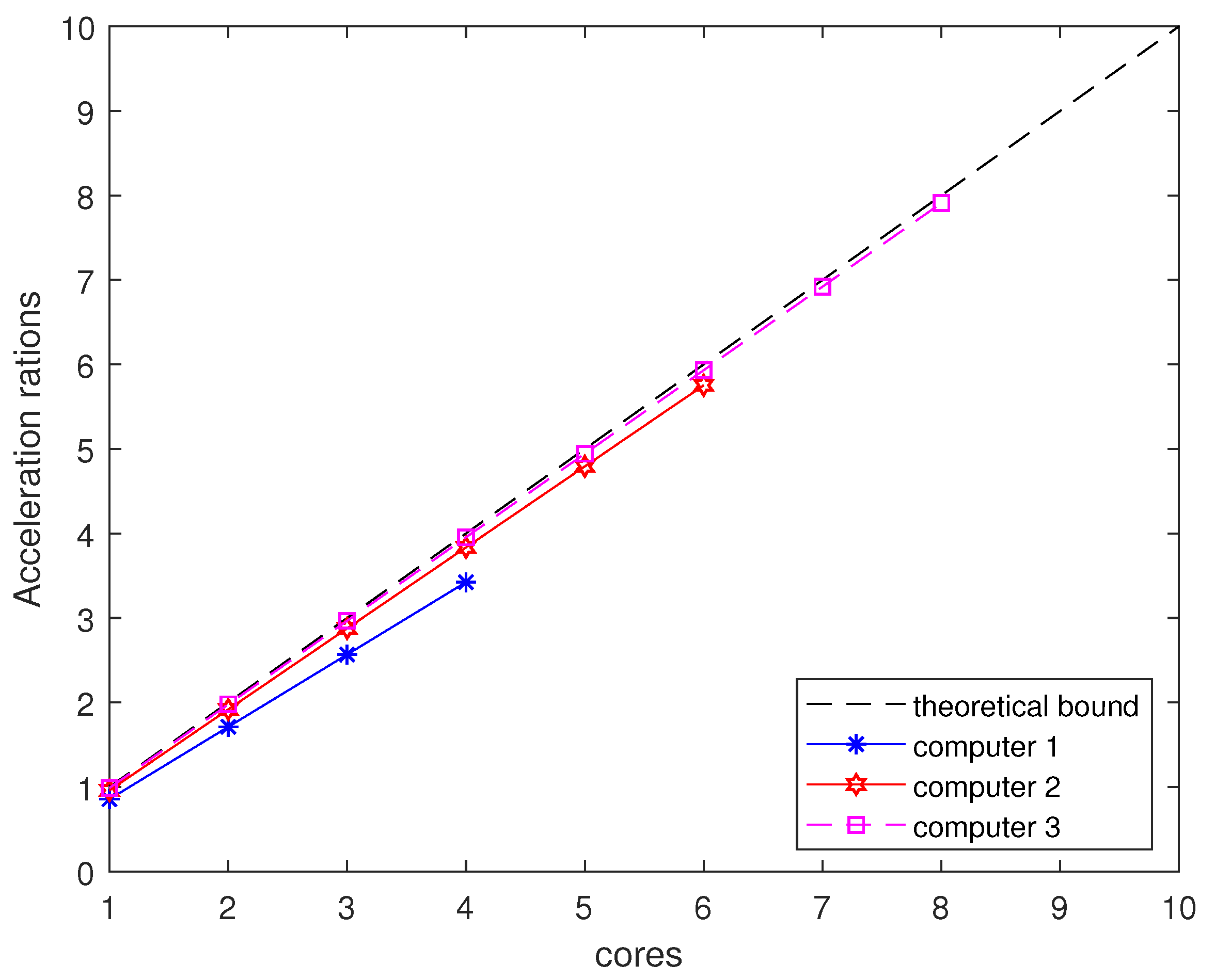
5.3.1. Parallel Implementation on Multicore Computers

Using a maximally splitting technique, the RLS problem can be maximally split into univariate sub-problems that can be executed in parallel, leading to a highly parallel structure.
To verify our theoretical analysis, experiments are conducted on the Gisette dataset on different multicore computers. The relationship between acceleration ratios and the number of cores is characterized by the acceleration ratio R, defined by the single-core runtime divided by the n-core runtime. The experiments are carried out on three multi-core computers. The hardware configurations of the three computers are, respectively, an Intel Core i7-10700 8-core CPU @ 2.9 GHz, an Intel Core i7-4790 4-core CPU @ 3.60 GHz, and an Intel Core i7-8700 6-core CPU @ 3.2 GHz.
The three computers are shown in Figure 4. From Figure 4, the relationship between the acceleration ratios and the number of CPU cores is close to the lower bound, demonstrating the high parallelism of the MS-ARADMM.

5.3.2. Parallel Implementation on GPU

As one of the important indexes to evaluate the convergence performance of the algorithm, the high parallel performance effectively alleviates the computational pressure and further improves the operation efficiency of the algorithm. Through internal multi-process parallel computing, the GPU can have a speed that is one order of magnitude higher than the CPU; it also has a strong ability of floating point arithmetics, which can greatly improve the computing speed of the ADMM and shorten the calculation time.
In case of high dimensional data, MI-based RELM requires a large amount of storage and computation. To verify the high parallelism of the algorithm, parallel accelerated experiments of MS-ARADMM-based and MI-based RELMs are realized on an NVIDIA GeForce GT 730 display card. The parallel implementations on the GPU are implemented by using the gpuArray function in the MATLAB toolbox.
The MS-ARADMM-based RELM splits the model-fitting problem into a set of univariate sub-problems that can be executed in parallel. Its convergence speed is improved by the parameter selection scheme. Theoretically, the MS-ARADMM has good convergence speed and parallelism.
The simulation results from all of the datasets are given in Table 5. From Table 5, on all the datasets except USPS, Pendigits, and Optical-Digits, the computational complexity of the MS-ARADMM-based RELM is much smaller than that of the MI-based RELM. On all of the datasets, the computational complexy of the MS-ARADMM-based RELM is much smaller than that of the MI-based RELM when implemented on the GPU. The acceleration ratio of the MI-based method is about 5.3443 , whereas that of the MS-ARADMM is about 23.5065 —an acceleration of four times that of the MI-based method.

5.4. Accuracy Analysis

The classification accuracy is an important indicator of classifier performance. Accuracy was compared on the MS-ARADMM-based, MS-AADMM-based, and MI-based RELMs.
Table 6 compares the training accuracy and the testing accuracy of the MS-ARADMM, the MS-AADMM, and the MI-based RELMs. From Table 6, we can see that the classification accuracy by the MS-ARADMM is not affected. From Table 3 and Table 6, under approximately identical training and the testing accuracy, the computational time for the MS-ARADMM is less than those of both the MI-based and the MS-AADMM-based methods. Thus, the convergence speed of MS-ARADMM is greatly improved in solving large-scale optimization problems.

6. Conclusions

In this paper, an MS-ARADMM algorithm is proposed to solve the RLS problem in the RELM. Its novelty is reflected in two aspects: (1) The non-monotonic Wolfe-type strategy is introduced into the memory gradient method to improve the global convergence; (2) The step selection constraint is added to simplify the computational complexity of MS-RADMM subproblems. Since the MS-ARADMM is a convex optimization method with superlinear global convergence, it can ensure a fast response and global optimal solution of the RELM, so it is more suitable to realize the distributed computation of large-scale convex optimization problems of the RELM compared with other ADMM methods.
We focused on the influences of parameters ρ and α on the convergence performance of the RELM model. To verify the performance of the proposed algorithms, we applied them to various large-scale classification datasets, and compared the simulation results with the methods implemented in Table 2 and Table 3. The results confirm that the computation efficiency of the RELM model is obviously improved, especially when applied to large-scale convex optimization problems. Therefore, the MS-ARADMM algorithm could enhance the convergence speed since it has a simpler solution process.

Author Contributions

Conceptualization, S.H. and Z.W.; methodology, Z.W.; writing—original draft preparation, S.H. and Z.W.; writing—review and editing, X.X., B.L. and K.W.; supervision, Z.W. and B.L.; project administration, Z.W. and K.W. All authors have read and agreed to the published version of the manuscript.

Funding

This work was supported in part by the Zhejiang Provincial “Ling Yan” Research and Development Program under Grant No. 2022C03122, in part by Public Welfare Technology Application and Research Program in Zhejiang Province under Grants No. LGF22F020006 and LQ23F030002, and in part by the Open Research Project of the State Key Laboratory of Industrial Control Technology, Zhejiang University under No. ICT2022B34.

Institutional Review Board Statement

Not applicable.

Informed Consent Statement

Not applicable.

Data Availability Statement

Not applicable.

Conflicts of Interest

The authors declare no conflict of interest.

References

  1. Zheng, Y.F.; Chen, B.D.; Wang, S.Y. Mixture Correntropy-Based Kernel Extreme Learning Machines. IEEE Trans. Neural Netw. Learn. Syst. 2022, 33, 811–825. [Google Scholar] [CrossRef] [PubMed]
  2. Deng, W.; Zheng, Q.; Chen, L. Regularized extreme learning machine. In Proceedings of the 2009 IEEE Symposium on Computational Intelligence and Data Mining, Nashville, TN, USA, 30 March–2 April 2009; pp. 389–395. [Google Scholar]
  3. Huang, G.B.; Zhu, Q.Y.; Siew, C.K. Extreme learning machine: Theory and applications. Neurocomputing 2006, 70, 489–501. [Google Scholar] [CrossRef]
  4. Shi, X.; Kang, Q.; An, J. Novel L1 Regularized Extreme Learning Machine for Soft-Sensing of an Industrial Process. IEEE Trans. Ind. Inform. 2022, 18, 1009–1017. [Google Scholar] [CrossRef]
  5. Wang, Y.; Dou, Y.; Liu, X. PR-ELM: Parallel regularized extreme learning machine based on cluster. Neurocomputing 2016, 173, 1073–1081. [Google Scholar] [CrossRef]
  6. Liu, P.; Wang, X.; Huang, Y. Research on Parallelization of Extreme Learning Machine Algorithm Based on Spark. Comput. Sci. 2017, 44, 33–37. [Google Scholar]
  7. Chen, C.; Li, K.; Ouyang, A. GPU-accelerated parallel hierarchical extreme learning machine on Flink for big data. IEEE Trans. Syst. Man Cybern. Syst. 2017, 47, 2740–2753. [Google Scholar] [CrossRef]
  8. Duan, M.; Li, K.; Liao, X. A parallel multi classification algorithm for big data using an extreme learning machine. IEEE Trans. Neural Netw. Learn. Syst. 2018, 29, 2337–2351. [Google Scholar] [CrossRef]
  9. Nagata, T.; Nonomura, T.; Nakai, K.; Yamada, K.; Saito, Y.; Ono, S. Data-Driven Sparse Sensor Selection Based on A-Optimal Design of Experiment with ADMM. IEEE Sens. J. 2021, 21, 15248–15257. [Google Scholar] [CrossRef]
  10. Li, Q.; Chen, B.; Yang, M. Improved Two-Step Constrained Total Least-Squares TDOA Localization Algorithm Based on the Alternating Direction Method of Multipliers. IEEE Sens. J. 2020, 20, 13666–13673. [Google Scholar] [CrossRef]
  11. Wang, H.; Feng, R.; Han, Z.F. ADMM-based algorithm for training fault tolerant RBF networks and selecting centers. IEEE Trans. Neural Netw. Learn. Syst. 2018, 29, 3870–3878. [Google Scholar]
  12. Wei, Y.; Li, Y.; Ding, Z. SAR Parametric Super-Resolution Image Reconstruction Methods Based on ADMM and Deep Neural Network. IEEE Trans. Geosci. Remote Sens. 2021, 59, 10197–10212. [Google Scholar] [CrossRef]
  13. Wang, H.; Gao, Y.; Shi, Y. Group-based alternating direction method of multipliers for distributed linear classification. IEEE Trans. Cybern. 2017, 47, 3568–3582. [Google Scholar] [CrossRef]
  14. Luo, M.; Zhang, L.; Liu, J. Distributed extreme learning machine with alternating direction method of multiplier. Neurocomputing 2017, 261, 164–170. [Google Scholar] [CrossRef]
  15. Bai, T.; Li, S.; Zou, Y. Distributed MPC for Reconfigurable Architecture Systems via Alternating Direction Method of Multipliers. IEEE/CAA J. Autom. Sin. 2021, 8, 1336–1344. [Google Scholar] [CrossRef]
  16. Xu, J.; Chen, X.; Hu, S. Low-bit Quantization of Recurrent Neural Network Language Models Using Alternating Direction Methods of Multipliers. In Proceedings of the ICASSP 2020—2020 IEEE International Conference on Acoustics, Speech and Signal Processing (ICASSP), Barcelona, Spain, 4–8 May 2020; pp. 7939–7943. [Google Scholar]
  17. Chen, C.; He, B.; Ye, Y.; Yuan, X. The direct extension of ADMM for multi-block convex minimization problems is not necessarily convergent. Math. Program. 2016, 155, 57–79. [Google Scholar] [CrossRef]
  18. Guo, K.; Han, D.; Wang, D.Z.; Wu, T. Convergence of ADMM for multi-block nonconvex separable optimization models. Front. Math. China 2017, 12, 1139–1162. [Google Scholar] [CrossRef]
  19. Han, D.; Yuan, X.; Zhang, W.; Cai, X. An ADM-based splitting method for separable convex programming. Comput. Optim. Appl. 2013, 54, 343–369. [Google Scholar] [CrossRef]
  20. Li, M.; Sun, D.; Toh, K.C. A convergent 3-block semi-proximal ADMM for convex minimization problems with one strongly convex block. Asia-Pac. J. Oper. Res. 2015, 32, 1550024. [Google Scholar] [CrossRef] [Green Version]
  21. Lai, X.; Cao, J.; Zhao, R. A Relaxed ADMM Algorithm for WLS Design of Linear-Phase 2D FIR Filters. In Proceedings of the 2018 IEEE 23rd International Conference on Digital Signal Processing (DSP), Shanghai, China, 19–21 November 2018; pp. 1–5. [Google Scholar]
  22. Lai, X.; Cao, J.; Huang, X. A Maximally Split and Relaxed ADMM for Regularized Extreme Learning Machines. IEEE Trans. Neural Netw. Learn. Syst. 2020, 31, 1899–1913. [Google Scholar] [CrossRef]
  23. Su, Y.; Xu, J.; Qin, H. Kernel Extreme Learning Machine Based on Alternating Direction Multiplier Method of Binary Splitting Operator. J. Electron. Inf. Technol. 2021, 43, 2586–2593. [Google Scholar]
  24. Ma, M.; Lai, X.; Meng, H. The Maximum Partition Relaxation ADMM Algorithm of Two-dimensional FIR Filter Constrained Least Square Design. Electron. J. 2020, 48, 510–517. [Google Scholar]
  25. Hou, X.; Lai, X.; Cao, J. A Maximally Split Generalized ADMM for Regularized Extreme Learning Machines. Electron. J. 2021, 49, 625–630. [Google Scholar]
  26. Qing, Y.; Zeng, Y.; Li, Y. Deep and wide feature based extreme learning machine for image classification. Neurocomputing 2020, 412, 426–436. [Google Scholar] [CrossRef]
  27. Li, R.; Wang, C.; Zhang, H. Using Wavelet Packet Denoising and a Regularized ELM Algorithm Based on the LOO Approach for Transient Electromagnetic Inversion. IEEE Trans. Geosci. Remote Sens. 2022, 60, 1–17. [Google Scholar] [CrossRef]
  28. Er, M.J.; Shao, Z.; Wang, N. A fast and effective Extreme learning machine algorithm without tuning. In Proceedings of the 2014 International Joint Conference on Neural Networks (IJCNN), Beijing, China, 6–11 July 2014; pp. 770–777. [Google Scholar]
  29. Zhao, Y.; Wang, K. Fast cross validation for regularized extreme learning machine. J. Syst. Eng. Electron. 2014, 25, 895–900. [Google Scholar] [CrossRef]
  30. Yan, S.; Yang, M. Alternating Direction Method of Multipliers with variable stepsize for Partially Parallel MR Image reconstruction. In Proceedings of the 36th Chinese Control Conference, Dalian, China, 26–28 July 2017. [Google Scholar]
  31. Song, H.; Zhang, B.; Wang, M. A Fast Phase Optimization Approach of Distributed Scatterer for Multitemporal SAR Data Based on Gauss-Seidel Method. IEEE Geosci. Remote Sens. Lett. 2022, 19, 1–5. [Google Scholar] [CrossRef]
  32. Sun, K.; Sun, X.A. A Two-Level ADMM Algorithm for AC OPF with Global Convergence Guarantees. IEEE Trans. Power Syst. 2021, 36, 5271–5281. [Google Scholar] [CrossRef]
  33. Yang, L.; Luo, J.; Xu, Y. A Distributed Dual Consensus ADMM Based on Partition for DC-DOPF with Carbon Emission Trading. IEEE Trans. Ind. Inform. 2019, 16, 1858–1872. [Google Scholar] [CrossRef]
  34. Huang, S.; Wu, Q.; Bao, W.; Hatziargyriou, N.D.; Ding, L.; Rong, F. Hierarchical Optimal Control for Synthetic Inertial Response of Wind Farm Based on Alternating Direction Method of Multipliers. IEEE Trans. Sustain. Energy 2021, 12, 25–35. [Google Scholar] [CrossRef]
  35. Luo, X.; Zhong, Y.; Wang, Z. An Alternating-Direction-Method of Multipliers-Incorporated Approach to Symmetric Non-Negative Latent Factor Analysis. IEEE Trans. Neural Netw. Learn. Syst. 2021, 16, 1–15. [Google Scholar] [CrossRef]
  36. Bastianello, N.; Carli, R.; Schenato, L. Asynchronous Distributed Optimization Over Lossy Networks via Relaxed ADMM: Stability and Linear Convergence. IEEE Trans. Autom. Control 2021, 66, 2620–2635. [Google Scholar] [CrossRef]
  37. Liang, X.; Li, Z.; Huang, W. Relaxed Alternating Direction Method of Multipliers for Hedging Communication Packet Loss in Integrated Electrical and Heating System. J. Mod. Power Syst. Clean Energy 2020, 8, 874–883. [Google Scholar] [CrossRef]
  38. Erseghe, T. New Results on the Local Linear Convergence of ADMM: A Joint Approach. IEEE Trans. Autom. Control 2021, 8, 5096–5111. [Google Scholar] [CrossRef]
  39. Xu, Z.; Figueiredo, M.; Goldstein, T. Adaptive ADMM with Spectral Penalty Parameter Selection. AISTATS 2017, 1, 1–7. [Google Scholar]
  40. Zhang, Z.H.; Shi, Z.H.J.; Wang, C.H.Y. A new memory gradient method and its convergence. Math. Econ. 2006, 23, 421–425. [Google Scholar]
  41. Xu, Z.; Figueiredo, M.A.T.; Yuan, X. Adaptive Relaxed ADMM: Convergence Theory and Practical Implementation. In Proceedings of the 2017 IEEE Conference on Computer Vision and Pattern Recognition (CVPR), Honolulu, HI, USA, 21–26 July 2017. [Google Scholar]
  42. Yu, T.; Liu, X.W.; Dai, Y.H. A Minibatch Proximal Stochastic Recursive Gradient Algorithm Using a Trust-Region-Like Scheme and Barzilai-Borwein Stepsizes. IEEE Trans. Neural Netw. Learn. Syst. 2021, 32, 4627–4638. [Google Scholar] [CrossRef] [PubMed]
  43. Du, K.-L.; Swamy, M.N.S.; Wang, Z.-Q.; Mow, W.H. Matrix Factorization Techniques in Machine Learning, Signal Processing, and Statistics. Mathematics 2023, 11, 2674. [Google Scholar] [CrossRef]
Figure 1. Illustration of the MS-ARADMM-based RELM.
Mathematics 11 03198 g001
Figure 2. Convergence comparison of different methods.
Mathematics 11 03198 g002
Figure 3. Convergence performance of RB-ADMM, MS-ADMM, and MS-ARADMM on different datasets. (a) BASEHOCK, (b) Gisette, (c) Magic, (d) Optical-Digits, (e) PCMAC, (f) Pendigits, (g) Satlag, (h) USPS.
Mathematics 11 03198 g003
Figure 4. Convergence of MS-ARADMM on three computers on Gisette dataset.
Mathematics 11 03198 g004
Table 1. Dataset specifications.
DatasetNumber of AttributesNumber of Training SamplesNumber of Testing SamplesNumber of Classes
Gisette5000560014002
USPS2567439185910
Magic1015,21638042
BASEHOCK486215954382
Pendigits168794219810
Optical-Digits644496112410
Statlog36514812876
PCMAC328915553882
Table 2. Comparison of iterations for different methods.
Termination Condition (Error)Iterations
MBBHNABBHMTBBHProposed
1 × 10 4 13411411778
1 × 10 6 18215412695
1 × 10 8 201178135115
1 × 10 10 274230176146
1 × 10 12 306270243194
Table 3. Comparison of the convergence speed of RELM for different algorithms.
DatasetRB-ADMMMS-AADMMMS-ARADMM
Time(s)Number of IterationsTime(s)Number of IterationsTime(s)Number of Iterations
Gisette737.524491233.4513395.95187
USPS2621.8914546152.57413133.94955
BASEHOCK332.813916749.0221411.53897
Magic1156.617867446.05992512.91157
Pendigits3912.3798742176.37533337.329817
Optical-Digits1825.9015538139.22354124.501735
Statlog1626.432270492.01773916.433011
PCMAC353.241417533.3102151.96769
Table 4. Comparison of convergence speed improvement of MS-ARADMM and different methods.
DatasetNumber of CategoriesMS-ARADMM Compared to RB-ADMMMS-ARADMM Compared to MS-AADMM
Gisette299.232482.0512
Magic299.581882.9268
BASEHOCK299.486572
PCMAC298.961440
statlog698.437571.7948
USPS1099.084283.8709
Pendigits1097.708848.4848
Optical-Digits1093.494414.6341
Table 5. GPU acceleration ratios.
DatasetMI-Based RELMMS-ARADMM-Based RELM
CPUGPUAcceleration RatioCPUGPUAcceleration Ratio
Gisette51.53139.8855.21316.35200.7158.8839
USPS50.140610.4874.781261.12832.58923.6108
BASEHOCK29.98445.5445.40841.27500.10711.9159
Magic78.750013.0936.017029.01341.53718.8766
Pendigits54.71889.2265.9309115.00153.04337.7921
Optical-Digits36.23446.5595.524444.79471.88123.8143
Statlog38.51568.7564.398834.58820.67551.2418
PCMAC27.96885.1035.48092.78720.23012.1183
Table 6. Training accuracy and testing accuracy.
DatasetMI-BasedMS-AADMMMS-ARADMM
TrainingTestingTrainingTestingTrainingTesting
Gisette99.160795.571499.607196.214399.160796.0714
USPS97.916197.043098.077496.559198.037196.9054
BASEHOCK90.586790.213389.585990.130391.091590.4111
Magic81.920381.861281.788981.756081.775781.7297
Pendigits96.702396.678896.565896.696896.520396.8148
Optical-Digits98.865798.398698.798997.864898.843497.9537
Statlog85.819782.517485.625582.750685.703182.5951
PCMAC99.485291.516799.356591.516799.742691.4602
Disclaimer/Publisher’s Note: The statements, opinions and data contained in all publications are solely those of the individual author(s) and contributor(s) and not of MDPI and/or the editor(s). MDPI and/or the editor(s) disclaim responsibility for any injury to people or property resulting from any ideas, methods, instructions or products referred to in the content.

