
Semi-Analytical Analysis of Drug Diffusion through a Thin Membrane Using the Differential Quadrature Method


Abstract
:1. Introduction
2. Formulation of the Problem
3. Method of Solution
3.1. Case 1
3.2. Case 2
- Shape Function 1: Lagrange Interpolation Polynomial (PDQM);
- Shape Function 2: Discrete Singular Convolution (DSCDQM)
- Kernel (1): Delta Lagrange Kernel (DLK):
- Kernel (2): Regularized Shannon kernel (RSK) [41]:
- Firstly, solving Equations (11) and (13) as a linear system;
- Case 1:
- Case 2:
- Case 1:
- Case 2:
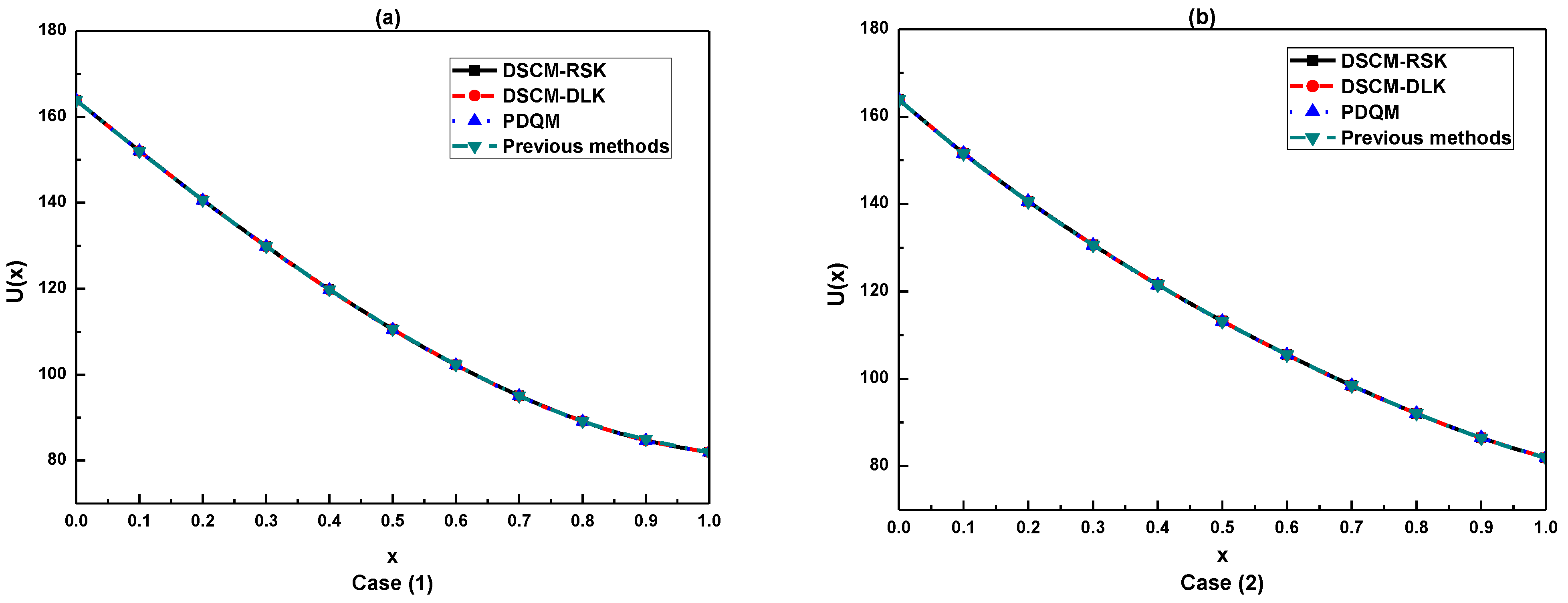
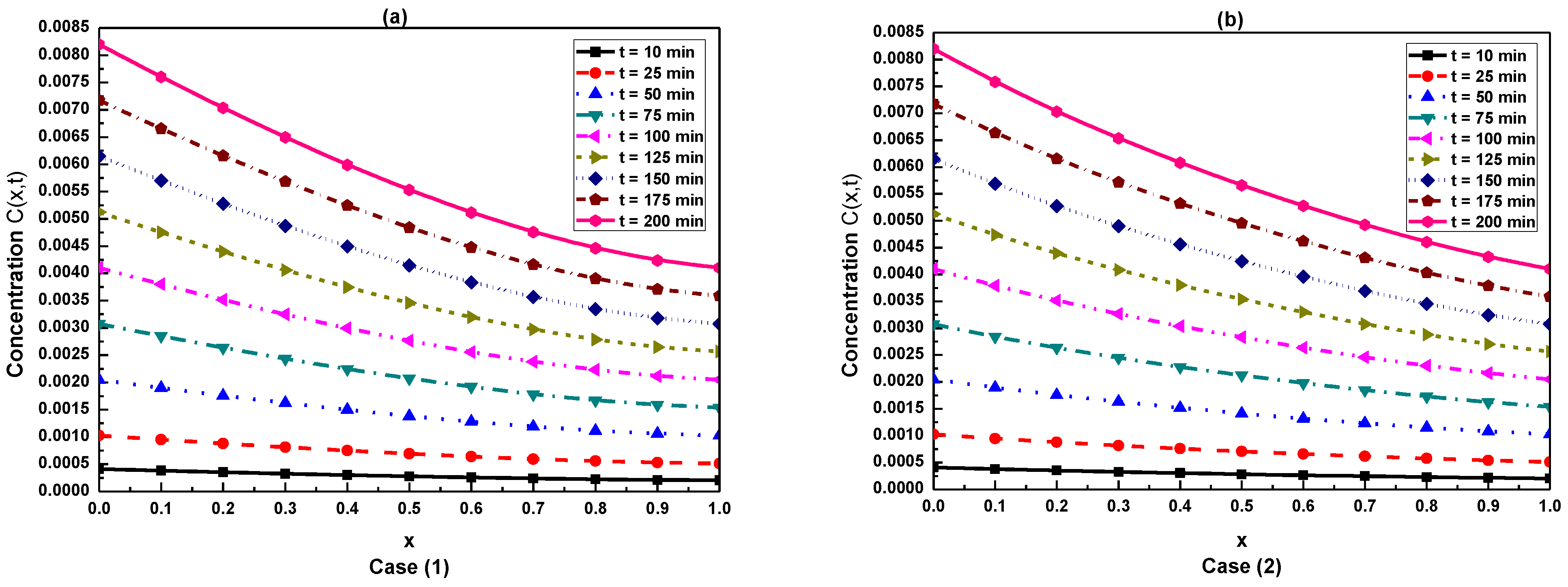
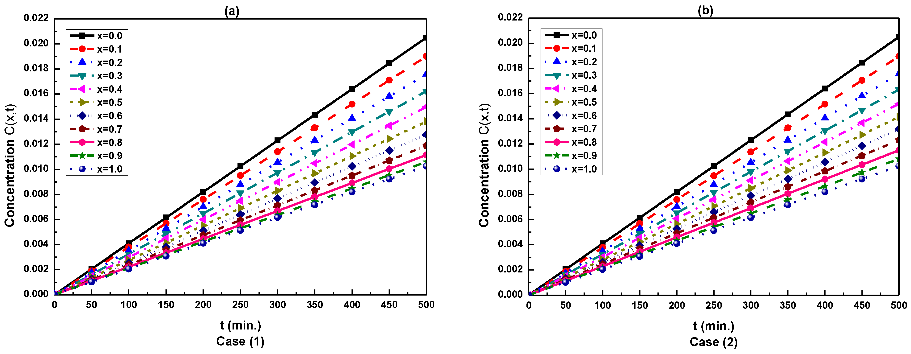
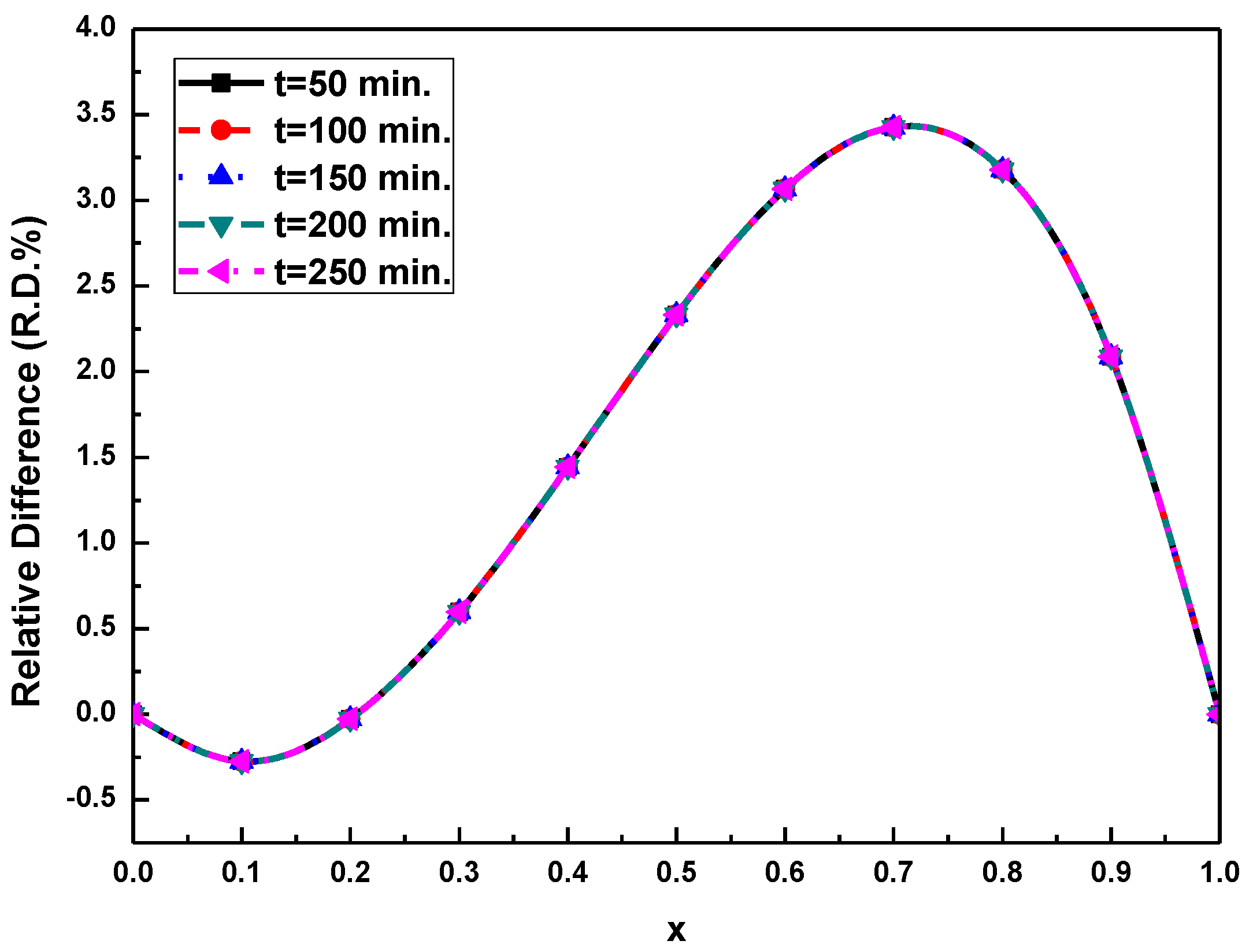
4. Numerical Results
5. Conclusions
- The computed results demonstrated that the concentration reduces slightly with distance and increases with time.
- The tiny relative differences in concentration for the two cases prove that the influence of the coefficient of diffusion is negligible.
- The value of R.D.% grows gradually toward x, reaching its highest value at x = 0.7, before decreasing to zero at x = 1.
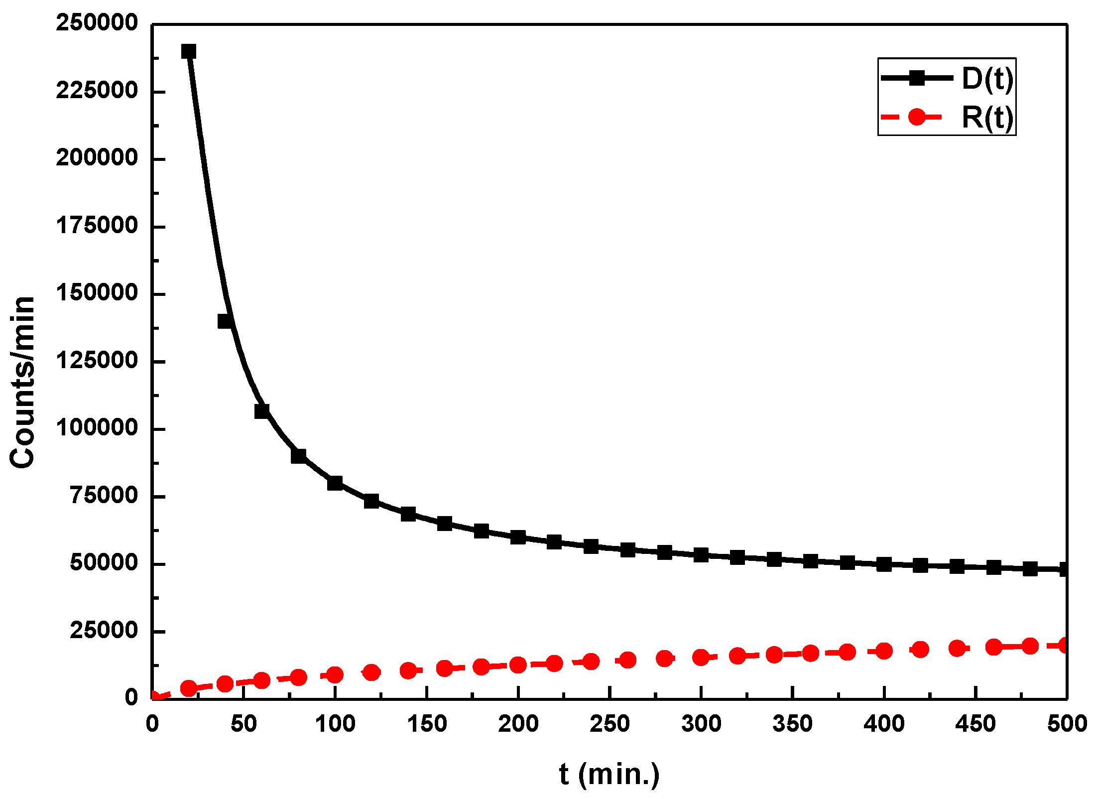
- The concentration in the donor cell D(t) decreases with time, while that in the recipient cell R(t) rises, which is consistent with the theoretical model.
Author Contributions
Funding
Data Availability Statement
Acknowledgments
Conflicts of Interest
References
- Hansen, S.; Lehr, C.-M.; Schaefer, U.F. Improved Input Parameters for Diffusion Models of Skin Absorption. Adv. Drug Deliv. Rev. 2013, 65, 251–264. [Google Scholar] [CrossRef] [PubMed]
- Špaček, P.; Kubin, M. Diffusion in Gels. J. Polym. Sci. Part C Polym. Symp. 1967, 16, 705–714. [Google Scholar]
- Hoogervorst, C.J.P.; Van Dijk, J.; Smit, J.A.M. Transient Diffusion through a Membrane Separating Two Unequal Volumes of Well Stirred Solution. CJP Hoogervorst, Non-Stationary Diffusion through Membranes. Ph.D. Thesis, Rijksuniversiteit te Leiden, Leiden, The Netherlands, 1977. [Google Scholar]
- Kasem, M.M.M. Group Theoretic Approach for Solving the Problem of Di# Usion of a Drug through a Thin Membrane; Elsevier: Amsterdam, The Netherlands, 2002; pp. 1–11. [Google Scholar]
- Spoelstra, J.; Van Wyk, D.J. A Method of Solution for a Non-Linear Diffusion Model and for Computing the Parameters in the Model. J. Comput. Appl. Math. 1987, 20, 379–385. [Google Scholar] [CrossRef] [Green Version]
- Hoelz, A.; Debler, E.W.; Blobel, G. The Structure of the Nuclear Pore Complex. Annu. Rev. Biochem. 2011, 80, 613–643. [Google Scholar] [CrossRef] [PubMed] [Green Version]
- Petrotos, K.B.; Lazarides, H.N. Osmotic Concentration of Liquid Foods. J. Food Eng. 2001, 49, 201–206. [Google Scholar] [CrossRef]
- Parisio, G.; Stocchero, M.; Ferrarini, A. Passive Membrane Permeability: Beyond the Standard Solubility-Diffusion Model. J. Chem. Theory Comput. 2013, 9, 5236–5246. [Google Scholar] [CrossRef]
- Nagle, J.F.; Mathai, J.C.; Zeidel, M.L.; Tristram-Nagle, S. Theory of Passive Permeability through Lipid Bilayers. J. Gen. Physiol. 2008, 131, 77–85. [Google Scholar] [CrossRef] [Green Version]
- Li, D.; Wang, H. Recent Developments in Reverse Osmosis Desalination Membranes. J. Mater. Chem. 2010, 20, 4551–4566. [Google Scholar] [CrossRef]
- Aho, V.; Mattila, K.; Kühn, T.; Kekäläinen, P.; Pulkkinen, O.; Minussi, R.B.; Vihinen-Ranta, M.; Timonen, J. Diffusion through Thin Membranes: Modeling across Scales. Phys. Rev. E 2016, 93, 43309. [Google Scholar] [CrossRef] [Green Version]
- Aidun, C.K.; Clausen, J.R. Lattice-Boltzmann Method for Complex Flows. Annu. Rev. Fluid Mech. 2010, 42, 439–472. [Google Scholar] [CrossRef]
- Benzi, R.; Succi, S.; Vergassola, M. The Lattice Boltzmann Equation: Theory and Applications. Phys. Rep. 1992, 222, 145–197. [Google Scholar] [CrossRef]
- Hansen, A.G. Similarity Analyses of Boundary Value Problems in Engineering; Prentice-Hall: Hoboken, NJ, USA, 1964. [Google Scholar]
- Gaggioli, R.A.; Moran, M.J. Group Theoretic Techniques for the Similarity Solution of Systems of Partial Differential Equations with Auxiliary Conditions; Wisconsin Univ Madison Mathematics Research Center: Madison, WI, USA, 1966. [Google Scholar]
- Boutros, Y.Z.; Abd-el-Malek, M.B.; Badran, N.A. Group Theoretic Approach for Solving Time-Independent Free-Convective Boundary Layer Flow on a Nonisothermal Vertical Flat Plate. Arch. Mech. Stosow. 1990, 42, 377–395. [Google Scholar]
- Abd-el-Malek, M.B.; El-Mansi, S.M.A. Group Theoretic Methods Applied to Burgers’ Equation. J. Comput. Appl. Math. 2000, 115, 1–12. [Google Scholar] [CrossRef] [Green Version]
- Abd-el-Malek, M.B.; Amin, A.M. Lie Group Analysis for Solving the Problem of Diffusion of Drugs across a Biological Membrane. J. Gen. Lie Theory Appl. 2015, 9, 1–4. [Google Scholar]
- Bellman, R.; Kashef, B.G.; Casti, J. Differential Quadrature: A Technique for the Rapid Solution of Nonlinear Partial Differential Equations. J. Comput. Phys. 1972, 10, 40–52. [Google Scholar] [CrossRef]
- Bellman, R.; Casti, J. Differential Quadrature and Long-Term Integration. J. Math. Anal. Appl. 1971, 34, 235–238. [Google Scholar] [CrossRef] [Green Version]
- Shu, C. Differential Quadrature and Its Application in Engineering; Springer Science & Business Media: Berlin/Heidelberg, Germany, 2012; ISBN 1447104072. [Google Scholar]
- Korkmaz, A.; Dağ, İ. Shock Wave Simulations Using Sinc Differential Quadrature Method. Eng. Comput. 2011, 28, 654–674. [Google Scholar] [CrossRef]
- Wei, G. Vibration Analysis by Discrete Singular Convolution. J. Sound Vib. 2001, 244, 535–553. [Google Scholar] [CrossRef]
- Nassar, M.; Matbuly, M.S.; Ragb, O. Vibration Analysis of Structural Elements Using Differential Quadrature Method. J. Adv. Res. 2013, 4, 93–102. [Google Scholar] [CrossRef]
- Ragb, O.; Matbuly, M.S.; Nassar, M. Analysis of Composite Plates Using Moving Least Squares Differential Quadrature Method. Appl. Math. Comput. 2014, 238, 225–236. [Google Scholar] [CrossRef]
- Salah, M.; Amer, R.M.; Matbuly, M.S. The Differential Quadrature Solution of Reaction-Diffusion Equation Using Explicit and Implicit Numerical Schemes. Appl. Math. 2014, 5, 42639. [Google Scholar] [CrossRef] [Green Version]
- Ragba, O.; Matbulya, M.S.; Nassarb, M. Quadrature Analysis of Functionally Graded Materials. Int. J. Eng. Technol. 2014, 14, 69–80. [Google Scholar]
- Matbuly, M.S.; Ragb, O.; Nassar, M. Natural Frequencies of a Functionally Graded Cracked Beam Using the Differential Quadrature Method. Appl. Math. Comput. 2009, 215, 2307–2316. [Google Scholar] [CrossRef]
- Osman, T.; Matbuly, M.S.; Mohamed, S.A.; Nassar, M. Analysis of Cracked Plates Using Localized Multi-Domain Differential Quadrature Method. Appl. Comput. Math. 2013, 2, 109–114. [Google Scholar] [CrossRef] [Green Version]
- Salah, M.; Amer, R.M.; Matbuly, M.S. Analysis of Reaction Diffusion Problems Using Differential Quadrature Method. Int. J. Eng. Technol. 2013, 13, 1–6. [Google Scholar]
- Ragb, O.; Mohamed, M.; Matbuly, M.S. Vibration Analysis of Magneto-Electro-Thermo NanoBeam Resting on Nonlinear Elastic Foundation Using Sinc and Discrete Singular Convolution Differential Quadrature Method. Mod. Appl. Sci. 2019, 13, 49. [Google Scholar] [CrossRef]
- Civalek, Ö. Free Vibration of Carbon Nanotubes Reinforced (CNTR) and Functionally Graded Shells and Plates Based on FSDT via Discrete Singular Convolution Method. Compos. Part B Eng. 2017, 111, 45–59. [Google Scholar] [CrossRef]
- Civalek, Ö.; Kiracioglu, O. Free Vibration Analysis of Timoshenko Beams by DSC Method. Int. J. Numer. Methods Biomed. Eng. 2010, 26, 1890–1898. [Google Scholar] [CrossRef]
- Wan, D.C.; Zhou, Y.C.; Wei, G.W. Numerical Solution of Incompressible Flows by Discrete Singular Convolution. Int. J. Numer. Methods Fluids 2002, 38, 789–810. [Google Scholar] [CrossRef]
- Zhang, L.; Xiang, Y.; Wei, G.W. Local Adaptive Differential Quadrature for Free Vibration Analysis of Cylindrical Shells with Various Boundary Conditions. Int. J. Mech. Sci. 2006, 48, 1126–1138. [Google Scholar] [CrossRef]
- Tornabene, F.; Fantuzzi, N.; Ubertini, F.; Viola, E. Strong Formulation Finite Element Method Based on Differential Quadrature: A Survey. Appl. Mech. Rev. 2015, 67, 020801. [Google Scholar] [CrossRef]
- Wei, G.W. Discrete Singular Convolution for the Solution of the Fokker–Planck Equation. J. Chem. Phys. 1999, 110, 8930–8942. [Google Scholar] [CrossRef]
- Shao, Z.; Wei, G.W.; Zhao, S. DSC Time-Domain Solution of Maxwell’s Equations. J. Comput. Phys. 2003, 189, 427–453. [Google Scholar] [CrossRef]
- Wang, X.; Yuan, Z.; Deng, J. A Review on the Discrete Singular Convolution Algorithm and Its Applications in Structural Mechanics and Engineering. Arch. Comput. Methods Eng. 2020, 27, 1633–1660. [Google Scholar] [CrossRef]
- Ragb, O.; Mohamed, M.; Matbuly, M.S. Free Vibration of a Piezoelectric Nanobeam Resting on Nonlinear Winkler-Pasternak Foundation by Quadrature Methods. Heliyon 2019, 5, e01856. [Google Scholar] [CrossRef] [Green Version]
- Ragb, O.; Mohamed, M.; Matbuly, M.S.; Civalek, O. An Accurate Numerical Approach for Studying Perovskite Solar Cells. Int. J. Energy Res. 2021, 45, 16456–16477. [Google Scholar] [CrossRef]


| Uniform | Non-Uniform | ||||||||
|---|---|---|---|---|---|---|---|---|---|
| Case 1 | Case 2 | Case 1 | Case 2 | Case 1 | Case 2 | Case 1 | Case 2 | ||
| 4 | 0.00235 | 0.00241 | 0.00325 | 0.00344 | 4 | 0.00167 | 0.00175 | 0.00259 | 0.00262 |
| 5 | 0.00201 | 0.00206 | 0.00211 | 0.00235 | 5 | 0.00087 | 0.00088 | 0.00237 | 0.00239 |
| 6 | 0.00138 | 0.00139 | 0.00198 | 0.00200 | 6 | 0.00071 | 0.00072 | 0.00140 | 0.00145 |
| 7 | 0.00099 | 0.00105 | 0.00145 | 0.00148 | 7 | 0.00069 | 0.00071 | 0.00138 | 0.00142 |
| 8 | 0.00072 | 0.00075 | 0.00140 | 0.00141 | 8 | 0.00069 | 0.00071 | 0.00138 | 0.00142 |
| 9 | 0.00069 | 0.00071 | 0.00138 | 0.00142 | 9 | 0.00069 | 0.00071 | 0.00138 | 0.00142 |
| 10 | 0.00069 | 0.00071 | 0.00138 | 0.00142 | 10 | 0.00069 | 0.00071 | 0.00138 | 0.00142 |
| 11 | 0.00069 | 0.00071 | 0.00138 | 0.00142 | 11 | 0.00069 | 0.00071 | 0.00138 | 0.00142 |
| Previous Studies [4,18] | 0.00069 | 0.00071 | 0.00138 | 0.00142 | 0.00069 | 0.00071 | 0.00138 | 0.00142 | |
| Execution time | 0.25 (second)—uniform | 0.013 (second)—non-uniform | |||||||
| PDQM | Previous Studies [4,18] | ||||||
|---|---|---|---|---|---|---|---|
| Case 1 | Case 2 | Case 1 | Case 2 | Case 1 | Case 2 | ||
| 0 | 163.9000 | 163.9000 | 0.0008195 | 0.0008195 | 0.000820 | 0.000820 | 5.0 × 10−07 |
| 0.1 | 151.9837 | 151.5689 | 0.0007599 | 0.0007584 | 0.000760 | 0.000758 | 1.0 × 10−07 |
| 0.2 | 140.5881 | 140.5502 | 0.00070294 | 0.0007028 | 0.000703 | 0.000703 | 1.0 × 10−07 |
| 0.3 | 129.8072 | 130.5885 | 0.000649 | 0.0006529 | 0.000650 | 0.000653 | 1.0 × 10−06 |
| 0.4 | 119.7429 | 121.4970 | 0.0005987 | 0.0006075 | 0.000600 | 0.000608 | 1.3 × 10−06 |
| 0.5 | 110.5066 | 113.1459 | 0.0005525 | 0.0005657 | 0.000553 | 0.000566 | 5.0 × 10−07 |
| 0.6 | 102.2230 | 105.4577 | 0.00051112 | 0.000528 | 0.000512 | 0.000528 | 8.8 × 10−07 |
| 0.7 | 95.0357 | 98.4086 | 0.00047518 | 0.000492 | 0.000476 | 0.000492 | 8.2 × 10−07 |
| 0.8 | 89.11420 | 92.0381 | 0.00044447 | 0.0004602 | 0.000446 | 0.000461 | 1.5 × 10−06 |
| 0.9 | 84.66554 | 86.47 | 0.00042333 | 0.0004325 | 0.000424 | 0.000433 | 6.7 × 10−07 |
| 1 | 81.9500 | 81.9500 | 0.00040975 | 0.00040975 | 0.000410 | 0.000410 | 2.5 × 10−07 |
| CPU (second) | 0.013 (second) | ||||||
| DSCDQM–DLK | DSCDQM–RSK | Previous Studies [4,18] | |||||||
|---|---|---|---|---|---|---|---|---|---|
| DLK | RSK | ||||||||
| 0.2 | 3 | 0.000813 | 0.000787 | 0.000763 | 0.000752 | 0.000726 | 0.000703 | 1 × 10⁻⁷ | 1 × 10⁻⁸ |
| 4 | 0.0007072 | 0.000729 | 0.000718 | 0.000711 | 0.000701 | ||||
| 5 | 0.0007031 | 0.000718 | 0.000709 | 0.000703 | 0.000698 | ||||
| 6 | 0.0007031 | 0.000718 | 0.000709 | 0.000703 | 0.000698 | ||||
| 0.4 | 3 | 0.0006274 | 0.000641 | 0.000635 | 0.000622 | 0.000629 | 0.000600 | 1 × 10⁻⁷ | 1 × 10⁻⁸ |
| 4 | 0.0006050 | 0.000631 | 0.000618 | 0.000608 | 0.000613 | ||||
| 5 | 0.0005999 | 0.000617 | 0.000608 | 0.000600 | 0.000595 | ||||
| 6 | 0.0005999 | 0.000617 | 0.000608 | 0.000600 | 0.000595 | ||||
| 0.6 | 3 | 0.0005333 | 0.000541 | 0.000532 | 0.000528 | 0.000525 | 0.000512 | 6 × 10⁻⁷ | 1 × 10⁻⁸ |
| 4 | 0.0005222 | 0.000537 | 0.000522 | 0.000517 | 0.000516 | ||||
| 5 | 0.0005114 | 0.000530 | 0.000518 | 0.000512 | 0.000507 | ||||
| 6 | 0.0005114 | 0.000530 | 0.000518 | 0.000512 | 0.000507 | ||||
| 0.8 | 3 | 0.0004529 | 0.000499 | 0.000472 | 0.000458 | 0.000449 | 0.000446 | 3 × 10⁻⁷ | 1 × 10⁻⁸ |
| 4 | 0.0004480 | 0.000480 | 0.000459 | 0.000450 | 0.000445 | ||||
| 5 | 0.0004457 | 0.000471 | 0.000452 | 0.000446 | 0.000441 | ||||
| 6 | 0.0004457 | 0.000471 | 0.000452 | 0.000446 | 0.000441 | ||||
| CPU (second) | 0.0115 (seconds) | 0.0108 (seconds) | |||||||
| DSCDQM–DLK | DSCDQM–RSK | Previous Studies [4,18] | |||||||
|---|---|---|---|---|---|---|---|---|---|
| R.D.% | R.D.% | R.D.% | |||||||
| Case 1 | Case 2 | Case 1 | Case 2 | Case 1 | Case 2 | ||||
| 0 | 0.004099 | 0.004099 | 0 | 0.00410 | 0.00410 | 0 | 0.00410 | 0.00410 | 0 |
| 0.1 | 0.003801 | 0.00379 | −0.29 | 0.00380 | 0.00379 | −0.26 | 0.00380 | 0.00379 | −0.26 |
| 0.2 | 0.003516 | 0.003515 | 0 | 0.00352 | 0.00352 | 0 | 0.00352 | 0.00352 | 0 |
| 0.3 | 0.003246 | 0.003266 | 0.61 | 0.00325 | 0.00327 | 0.61 | 0.00325 | 0.00327 | 0.61 |
| 0.4 | 0.002994 | 0.003038 | 1.44 | 0.00300 | 0.00304 | 1.315 | 0.00300 | 0.00304 | 1.315 |
| 0.5 | 0.002763 | 0.002829 | 2.33 | 0.00276 | 0.00283 | 2.33 | 0.00276 | 0.00283 | 2.33 |
| 0.6 | 0.002556 | 0.002637 | 3.07 | 0.00256 | 0.00264 | 3.03 | 0.00256 | 0.00264 | 3.03 |
| 0.7 | 0.002376 | 0.002461 | 3.45 | 0.00238 | 0.00246 | 3.25 | 0.00238 | 0.00246 | 3.25 |
| 0.8 | 0.002228 | 0.002302 | 3.21 | 0.00223 | 0.00230 | 3.18 | 0.00223 | 0.00230 | 3.18 |
| 0.9 | 0.002117 | 0.002162 | 2.08 | 0.00212 | 0.00216 | 2.08 | 0.00212 | 0.00216 | 2.08 |
| 1 | 0.002049 | 0.002049 | 0 | 0.00205 | 0.00205 | 0 | 0.00205 | 0.00205 | 0 |
| Case 1 | Case 2 | R.D.% | Case 1 | Case 2 | R.D.% | Case 1 | Case 2 | R.D.% | |
|---|---|---|---|---|---|---|---|---|---|
| 0 | 0.00102 | 0.00102 | 0 | 0.00205 | 0.00205 | 0 | 0.00307 | 0.00307 | 0 |
| 0.1 | 0.00095 | 0.00095 | 0 | 0.0019 | 0.0019 | 0 | 0.00285 | 0.00284 | −0.35 |
| 0.2 | 0.00088 | 0.00088 | 0 | 0.00176 | 0.00176 | 0 | 0.002637 | 0.00264 | 0.11 |
| 0.3 | 0.00081 | 0.00082 | 1.22 | 0.001623 | 0.00163 | 0.43 | 0.002435 | 0.00245 | 0.61 |
| 0.4 | 0.00075 | 0.00076 | 1.32 | 0.00150 | 0.00152 | 1.32 | 0.002246 | 0.00228 | 1.49 |
| 0.5 | 0.00069 | 0.00071 | 2.82 | 0.00138 | 0.00142 | 2.82 | 0.002073 | 0.00212 | 2.22 |
| 0.6 | 0.00064 | 0.00066 | 3.03 | 0.00128 | 0.00132 | 3.03 | 0.001918 | 0.00198 | 3.13 |
| 0.7 | 0.00059 | 0.00062 | 4.84 | 0.00119 | 0.00123 | 3.25 | 0.001783 | 0.00185 | 3.62 |
| 0.8 | 0.00056 | 0.00058 | 3.45 | 0.00111 | 0.00115 | 3.48 | 0.001672 | 0.00173 | 3.35 |
| 0.9 | 0.00053 | 0.00054 | 1.85 | 0.00106 | 0.00108 | 1.85 | 0.001588 | 0.00162 | 1.98 |
| 1 | 0.00051 | 0.00051 | 0 | 0.00102 | 0.00102 | 0 | 0.001537 | 0.001537 | 0 |
Disclaimer/Publisher’s Note: The statements, opinions and data contained in all publications are solely those of the individual author(s) and contributor(s) and not of MDPI and/or the editor(s). MDPI and/or the editor(s) disclaim responsibility for any injury to people or property resulting from any ideas, methods, instructions or products referred to in the content. |
© 2023 by the authors. Licensee MDPI, Basel, Switzerland. This article is an open access article distributed under the terms and conditions of the Creative Commons Attribution (CC BY) license (https://creativecommons.org/licenses/by/4.0/).
Share and Cite
Mustafa, A.; Salama, R.S.; Mohamed, M. Semi-Analytical Analysis of Drug Diffusion through a Thin Membrane Using the Differential Quadrature Method. Mathematics 2023, 11, 2998. https://doi.org/10.3390/math11132998
Mustafa A, Salama RS, Mohamed M. Semi-Analytical Analysis of Drug Diffusion through a Thin Membrane Using the Differential Quadrature Method. Mathematics. 2023; 11(13):2998. https://doi.org/10.3390/math11132998
Chicago/Turabian StyleMustafa, Abdelfattah, Reda S. Salama, and Mokhtar Mohamed. 2023. "Semi-Analytical Analysis of Drug Diffusion through a Thin Membrane Using the Differential Quadrature Method" Mathematics 11, no. 13: 2998. https://doi.org/10.3390/math11132998