1. Introduction
Plankton are floating organisms that provide a food source for other organisms ranging from shellfish to whales. As such, they play a crucial role in aquatic foodwebs [
1]. Phytoplankton are organisms, such as algae, which carry out photosynthesis and are an important means of carbon storage in the ocean [
2]. Zooplankton feed on phytoplankton or other zooplankton and include insect larvae and jellyfish. Due to their fundamental role in aquatic ecosystems and their influence on the global carbon cycle, it is important to understand the temporal dynamics of plankton ecosystems.
A variety of different models have been proposed for plankton ecosystems, emphasizing different aspects of these complex systems [
3,
4,
5,
6,
7,
8,
9,
10,
11]. Here, we study a model due to Kloosterman et al. [
12], which focussed on two aspects. The chemical nutrients in the system are recycled, thus the system is closed—the total amount of nutrient remains constant. This recycling takes time (e.g., due to decomposition of dead organisms) and thus the model should include a time delay. Both are important features of plankton ecosystems that lead to interesting mathematics.
The model of Kloosterman et al. [
12] is called an NPZ model as it is a system with three compartments, representing the dissolved nutrient (
N ), the amount of phytoplankton (
P), and the amount of zooplankton (
Z). It is described by the following equations:
Here, and g are positive parameters representing biological properties while is an appropriate distribution representing the time delay in nutrient recycling.
The function
f stands for the phytoplankton nutrient uptake as a function of the available nutrient and it has the following properties [
4]:
Similarly, the function
h stands for the available phytoplankton and it must satisfy conditions [
13,
14]:
Kloosterman et al. [
12] investigated how this model for a planktonic ecosystem is affected by the quantity of biomass it contains and by the delay distribution. They described the existence of the equilibrium points and gave some stability results for a general distribution function, using methods as in [
15]. Other stability results considered particular cases of the distribution function and relied primarily on numerical work.
In this study, we assume that the delay follows a gamma distribution function, with either one or two degrees of freedom, as these numbers of freedom degrees correspond to the biological data. We derive two models, described by systems of ordinary differential equations (ODEs), and analyse how the local stability and local bifurcation of the equilibrium points depend on the amount of total nutrients and on the mean delay of the distribution.
For the numerical simulations we have used a Holling type II functional response for
f,
with
For function
h, we used either a Holling Type II functional response
or a Holling Type III response
with
Using this delay, we have extended the results obtained in [
12].
2. The Models
Consider
the gamma distribution of mean
, with
k degrees of freedom:
Starting from system (
1) and using the gamma distribution function for the cases
and
, and some appropriate new variables, we derive two models, described by systems of ordinary differential equations (ODEs), without explicit delay. This reduction is often called the linear chain trick [
16,
17,
18].
For the case , we obtain a 4-dimensional system of ODEs, which is then reduced to a three-dimensional one. This will be called the weak model.
For , we obtain a five-dimensional system of ODEs that can be reduced to a four-dimensional system, which will be called the strong model.
2.1. The Weak Model
If
we have
for
Denoting
the equation describing the evolution of the dissolved nutrient
N can be written as:
In addition, using the change of variable
we have:
With the change of variable
we have
Thus, we obtain a 4D model (
), called “the weak model” in the following, described by
Since the conservation law
is fulfilled, we obtain
The substitution
leads to the following reduced 3D system:
with the phase space
2.2. The Strong Model
If the number of freedom degrees is
we have
for
Denoting
the equation describing the evolution of the dissolved phytoplankton nutrient from (
1) reads:
In addition, using the change of variable
we have
Thus, we obtain the following 5D model
, also called “the strong model”:
Obviously, the conservation law
is fulfilled, so we can substitute
leading to the following reduced 4D system of ordinary differential equations (ODE):
with the phase space
Also, for consistency, the initial conditions of the ODE model must satisfy
2.3. The Model without Delay
In the absence of delay, the model (
1) is described by the following equations:
Using conservation law
this system can be reduced to the following 2D system:
with the phase space
In the following, shall denote the biomass of the model. Thus, when referring to the model without delay , for the weak model , while for the strong model .
3. Equilibrium Solutions
In this section, we determine the stationary solutions of the two reduced systems (
7) and (
15), for the NPZ model with delayed gamma distribution, with one or two degrees of freedom. These solutions correspond to the equilibrium points of the corresponding dynamical systems.
Each of the three systems has at most three equilibrium points în the region of interest, namely:
- -
A trivial equilibrium , with no phytoplankton and no zooplankton;
- -
An equilibrium with phytoplankton and no zooplankton, denoted ;
- -
An equilibrium with both phytoplankton and zooplankton, denoted .
These equilibria may coexist for certain values of the total nutrients. The same property is valid for the reduced 2D system (
18) for the NPZ model without delay.
3.1. Equilibrium Points for the System without Delay
In [
12], it is shown that under the assumptions
system (
18) has at most three equilibrium points in
depending on the value of the total nutrient
Denoting as
the equilibrium points of system (
18) are
for all
with
for all
and
with
and
unique solution of the equation
for all
with
3.2. Equilibrium Points for the Reduced Weak System (7)
The system (
7) possesses at most three equilibria with the first three coordinates non-negative, solutions of the system
It follows that the trivial equilibrium is
The equilibrium with only phytoplankton is
with
Taking into account the properties of
if the condition
is satisfied (that is the growth rate of the plankton must be greater than the death rate), then there exists an unique
namely
satisfying this condition. From the first equation we obtain
while from the conservation law we obtain
This equilibrium is in the domain of interest if and only if Note that if then
The equilibrium with both phyto- and zooplankton is
with
from the third equation in (
23). If condition
is satisfied, then there exists an unique
such that
namely
and
The condition
must be satisfied in order to have
As
f is an increasing function, it follows that
and using the first equation of system (
23) we have
To show that there exists an
such that
is satisfied, consider the function
It follows that and As F is an increasing function, there exists an unique value such that
Denote, as in [
12],
Remark that
. As a consequence, the third equilibrium point
exists in
and is uniquely determined by (
30) if the conditions
and (
20) are satisfied. Note that if
then
The transitions between the equilibrium points will be discussed further in
Section 5.
Finally, we note that if
is an equilibrium of system (
7), then
with
is an equilibrium point for system solution of system (
6) and conversely.
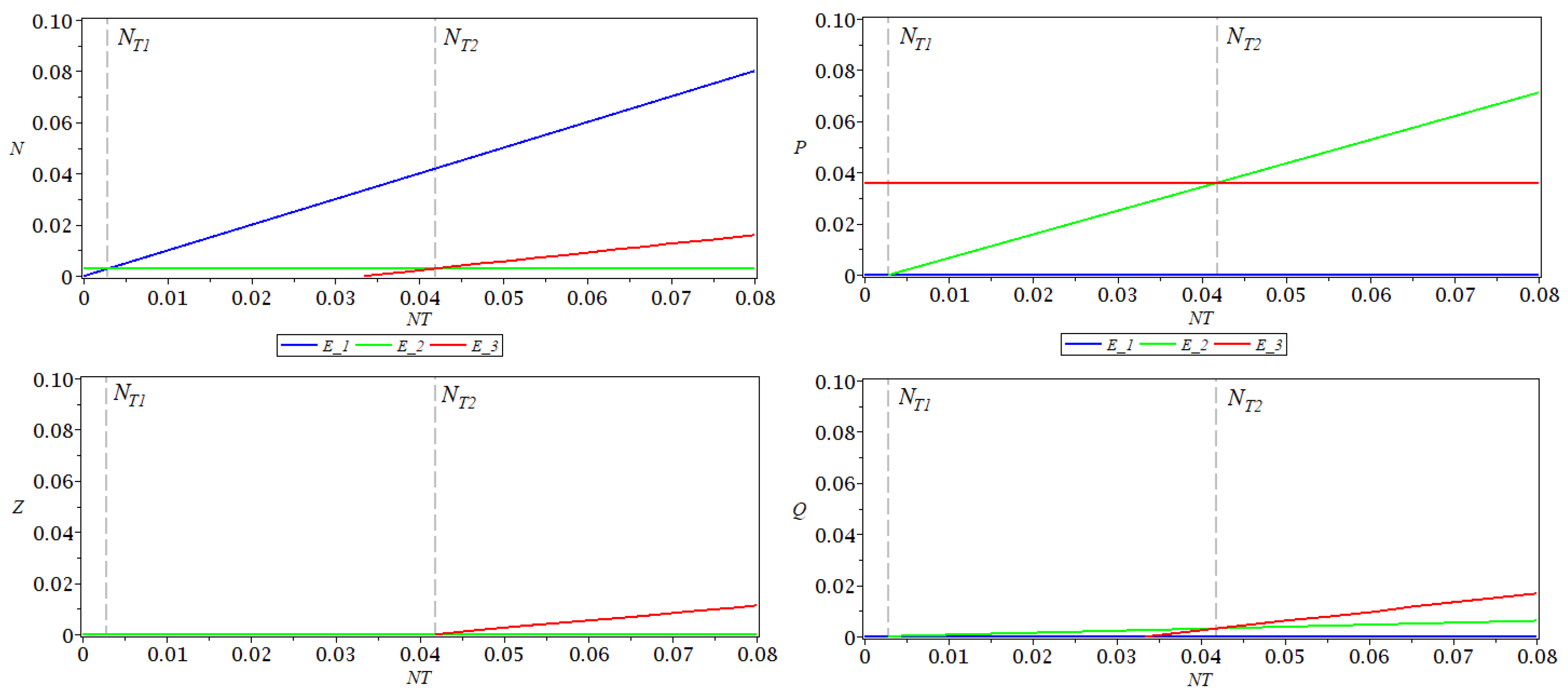
In
Figure 1, the coordinates
of the three equilibrium points are represented as functions of the total nutrient
, for a fixed
. As function
h, a type II functional response was considered. The values of the parameters used for simulations are
,
,
,
,
,
,
, as in [
12]. For these values of the parameters, the following values where obtained for thresholds:
,
.
3.3. Equilibria for the Reduced Strong Model (15)
The equilibria of system (
15) correspond to the solutions of the system
Substituting
from the first equation into the last equation in (
31), the remaining three equations coincide with system (
23). Consequently, we obtain the same expressions for
and
Z as for system (
23). Taking into account (
32), we obtain the following equilibrium points for system (
15):
- (1)
The trivial equilibrium for all
- (2)
The equilibrium with no zooplankton with
for all , with if ;
- (3)
The equilibrium , with
for all with if and .
Note that if
is an equilibrium of system (
15), then
is an equilibrium point for system solution of system (
13) and conversely.
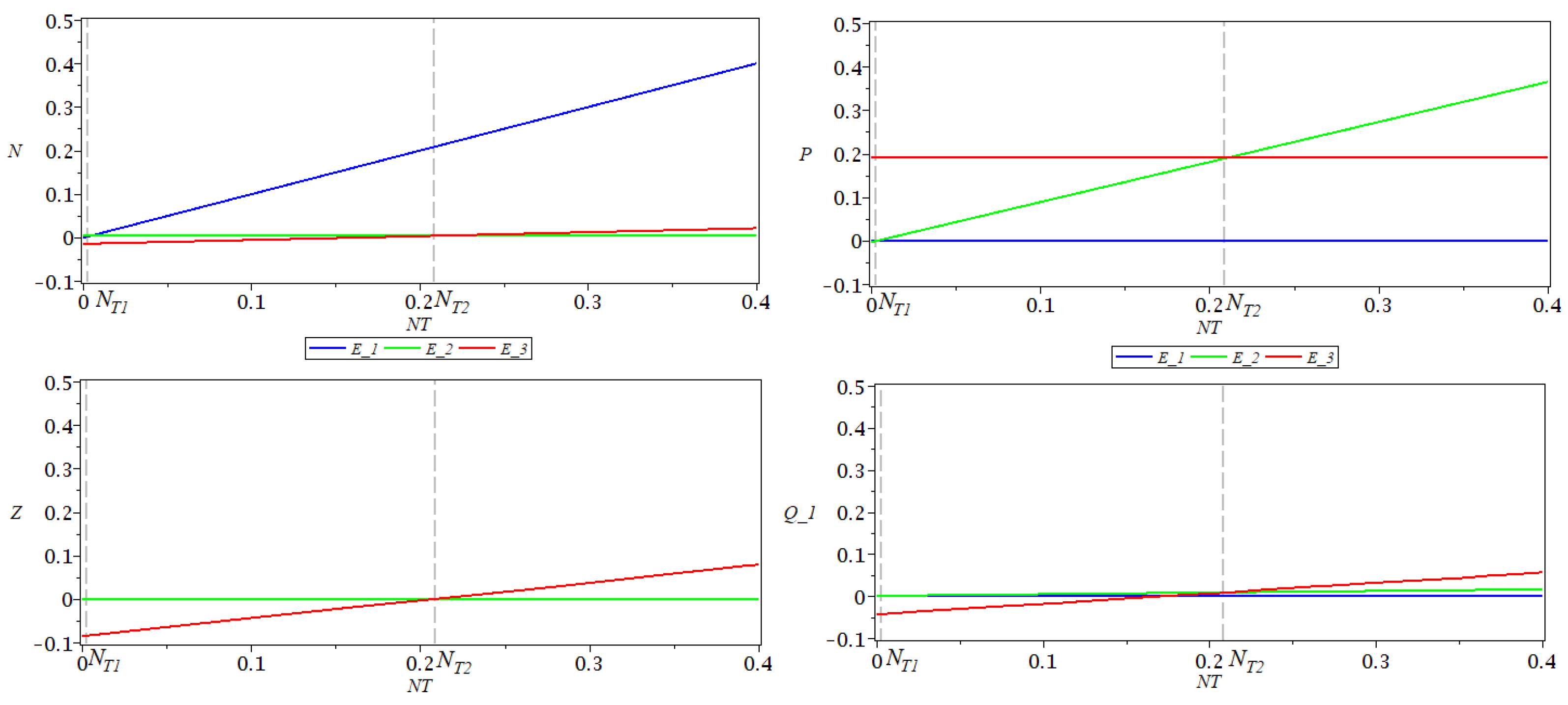
In
Figure 2, there are represented the coordinates
of the three equilibrium points as functions of the total nutrient
, for a fixed
. As function
h, a type III functional response was considered. The values of the parameters used for simulations are
,
,
,
,
,
,
, as in [
12]. For these values of the parameters, the following values were obtained for stability thresholds:
,
,
. Remark that
at
and
at
.
Comparing the systems with and without delay, we see the following.
The equilibrium point is unaffected by the delay.
For the equilibrium point , the value of P is reduced by the delay.
For the equilibrium point , the values of N and Z are reduced by the delay.
The first transition point is unaffected by the delay, while the second transition point is increased by the delay, if
4. Local Stability
For all three systems (
7), (
15) and (
18), we find that at each value of the total nutrient at most one of the equilibrium points is locally asymptotically stable. More precisely,
for the only equilibrium point is and it is asymptotically stable,
for the equilibrium is asymptotically stable, while is unstable,
and, finally, as the equilibrium is asymptotically stable either for all or there exists an such that is asymptotically stable for , and unstable for depending on the response function while the other two equilibria are unstable.
Note that for the system without delay (
18),
is equal to
. Our results for
and
reproduce the results of [
12] for the system with general delay (
1), while our results for
improve those of [
12].
Note that, for the two-dimensional reduced system without delay (
18), the local stability of the equilibria on the boundary of the domain can be extended to global stability [
12]. Those arguments cannot apply for systems (
7) and (
15). Results on the global stability could be obtained using Lyapunov functions, if they can be constructed.
4.1. The System without Delay
In [
12], it is shown that the equilibrium
is globally asymptotically stable on
if
the equilibrium
is globally asymptotically stable on
except for the
z axis, if
while the stability of the equilibrium point
depends on the sign of the quantity
denoting the trace of the Jacobi matrix
at
Here, to simplify the expression, we denoted ,
They proved that if
then the equilibrium point
is stable for all
This is valid for a type III zooplankton grazing response function
While if
then there exists a unique value
of the total nutrient, such that the equilibrium point
is asymptotically stable for all
and unstable if
The value
is found as the unique solution of the equation
with
For
the Jacobi matrix
has the purely imaginary eigenvalues
with
Close to
we have
Consequently,
and thus the transversality condition in the Hopf bifurcation theorem is satisfied. A Hopf bifurcation takes place for
if the Lyapunov coefficient
is non-zero.
4.2. The Weak Model Case
We analyse here the stability of the equilibrium points for the system (
7) corresponding to the gamma distribution delay, with one degree of freedom.
Proposition 1. For the equilibrium point of system (7), the following statements hold: - (i)
If , then is locally asymptotically stable in ;
- (ii)
If , then is a (2,1) type saddle point;
- (iii)
If , then is a fold singularity.
Proof. The Jacobian matrix
associated to system (
7) at
has the eigenvalues
As two eigenvalues are negative, the topological type of is determined by the sign of Thus, the equilibrium point is an attractor if , i.e., As f is an increasing function, we have if □
Proposition 2. The equilibrium point of system (7) is locally asymptotically stable in if and only if In addition,
- (i)
if or then is a fold singularity;
- (ii)
if then is a saddle point of type (2,1);
- (iii)
if then is not in
Proof. For the equilibrium
we obtain the Jacobi matrix
and the characteristic equation
with
Thus, one eigenvalue is
and we have
if
(that is
as
h is an increasing function). Consequently,
iff
and
if
.
The other two eigenvalues are solutions of the equation Further, if it follows that both solutions of this equation have negative real parts. As a consequence, if , all eigenvalues have negative real parts, hence the equilibrium point is an attractor.
Note that if then thus and The equilibrium point is a fold singularity both at and . □
For the equilibrium point
of system (
7), the Jacobi matrix reads
where, to simplify computation, we denoted:
Thus, the characteristic polynomial of
reads
with
Using the Routh–Hurwitz criterion [
19], all the roots of the characteristic polynomial have negative real parts if and only if the following conditions are satisfied:
Thus, the equilibrium point
is asymptotically stable if all these conditions are fulfilled. In [
12], one result on the stability of
with the weak gamma distributed delay was obtained. For completeness and for comparison with the strong gamma distribution case, we repeat that result here with proof.
Proposition 3. Ifthen the equilibrium of system (7) is locally asymptotically stable for all Proof. The equilibrium point
is stable if all conditions in (
38) are fulfilled. To simplify computation, denote
Note that,
. With these notations, we can write
As all parameters are positive, it follow that
As
conditions
and
are satisfied. As
condition (iii) in (
38) is satisfied. Consequently, all eigenvalues have negative real parts, and
is an attractor for all
□
Proposition 4. Ifthe following assertions hold for the equilibrium point of system (7). - (i)
For close to the equilibrium point is an attractor.
- (ii)
If , then is locally asymptotically stable.
- (iii)
If then is a Hopf singularity.
- (iv)
If then is a (1,2) saddle point. In addition, for each τ there exists a value given by
such that is locally asymptotically stable for all and unstable for close to
Proof. (i) The coefficient
is equal to 0 if and only
, which occurs when
The discussion following (
29) then shows that
at
and
for
For
the other two coefficients of the characteristic equation associated to
,
have positive values, and also
As the expressions
are continuous functions of
they remain positive for
in a neighbourhood of
Hence (i).
(ii) Considering
as a function of
we obtain
Differentiating with respect to
in (
30), we obtain
hence
As
and
, it follows that
thus
is a decreasing function of
Consequently,
The result follows by applying the Routh–Hurwitz criterion [
19].
(iii) The characteristic polynomial (
36) has a pair of purely imaginary roots
if conditions
As for all if then . Thus, is a Hopf singularity.
(iv) As for all and it follows that is the minimum value of for which condition is not satisfied. □
For the type II response function
h, we have
In this case, Proposition 4 applies for the stability of the equilibrium point
See
Figure 3.
For the type III response function
h, we obtain
In this case, if (i.e., then and the equilibrium point is stable for all If then Proposition 4 applies for the stability of the equilibrium point
4.3. The Strong Model Case
Proposition 5. The following assertions hold for the equilibrium point of system (15). - (i)
If , then is locally asymptotically stable in
- (ii)
If , then is a (3,1) type saddle point.
- (iii)
If , then is a fold singularity.
Proof. For the equilibrium
, we obtain the Jacobi matrix
and the characteristic polynomial
Thus,
has the eigenvalues
As three eigenvalues are negative, the topological type of is determined by the sign of Thus, the equilibrium point is an attractor if , i.e., As f is an increasing function, we obtain if □
Proposition 6. The equilibrium of system (15) is locally asymptotically stable in if and only if In addition,
- (i)
If or , then the equilibrium is a fold singularity;
- (ii)
If , then the equilibrium is a saddle point of type (3,1);
- (iii)
If , then the equilibrium is not in
Proof. For the equilibrium
we obtain the Jacobi matrix
and the characteristic equation
with
Thus, one eigenvalue is
and we have
if
(that is
as
h is an increasing function). Consequently,
if
and
as
The other three eigenvalues
are solutions of the equation
According to the Routh–Hurwitz criterion, all solutions of this equation have negative real parts if conditions
are fulfilled. As all parameters
are positive, if
the first two conditions
are satisfied. A simple computation shows that the third condition is also satisfied if
As a consequence, if
all eigenvalues have negative real part, hence the equilibrium point
is an attractor.
Note that if then thus and The equilibrium point is a fold singularity both at and . □
For the equilibrium
of system (
15), the Jacobi matrix reads
and the characteristic polynomial is
with
Using the Routh–Hurwitz criterion [
19], all the roots of the characteristic polynomial have negative real parts if and only if the following conditions are satisfied:
Thus, the equilibrium point is stable if all these conditions are fulfilled.
Proposition 7. For the equilibrium point of system (15), the following assertions hold. - (i)
For close to the equilibrium point is an attractor.
- (ii)
If one of the conditions , in (44) is not satisfied, then is unstable. In addition, for each τ there exists a value given by
such that is locally asymptotically stable for all
Proof. The coefficient is equal to 0 if and only Thus, we have at and for
At
the other three coefficients of the characteristic equation associated with
have the following values:
As the expressions
are continuous functions of
they remain positive for
in a neighbourhood of
Hence (i). Obviously,
is the minimum value of
for which one of the conditions (
44) is not satisfied. □
Remark 1. As for we have none of the eigenvalues can be 0. Thus, the topological type of could change only with the appearance of a pair of purely imaginary eigenvalues. Using the Viète relations, if conditionsare satisfied, then the equilibrium point is a Hopf singularity. Ifthen the equilibrium point has two pairs of purely imaginary eigenvalues and it is a double-Hopf singularity. Proposition 8. - (i)
If then the equilibrium of system (15) is locally asymptotically stable for all - (ii)
If then is a Hopf singularity.
- (iii)
If then is unstable. In addition, for each τ, there exists a value given by
such that is locally asymptotically stable for all
Proof. The equilibrium point
is stable if all conditions in (
38) are fulfilled. To simplify computation, denote:
Note that,
. With these notations, we can write:
As all parameters are positive, it follow that
As
conditions
are satisfied if the hypothesis (
47) is true. As
condition
is satisfied if (
47).
Consequently, if then all eigenvalues have negative real parts, thus is an attractor.
If
at least two eigenvalues have negative real parts, thus
is unstable. As for
we have
the expression continue to be positive for
close to
Obviously,
is the minimum value of
for which
□
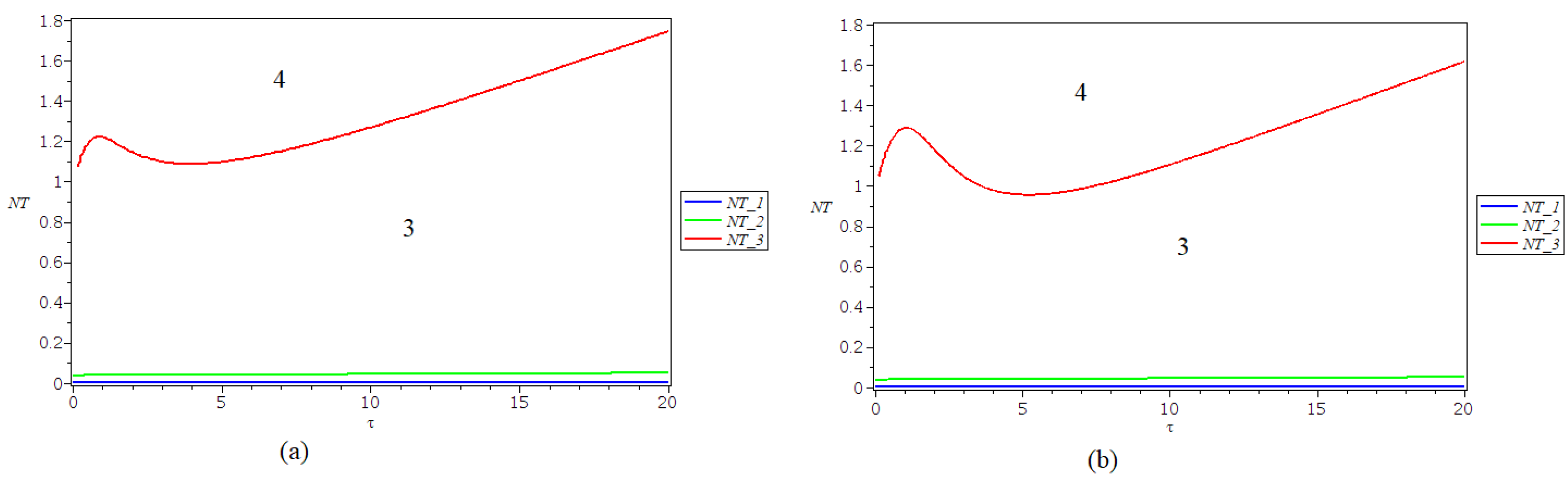
In
Figure 3, there are represented the strata in the
plane that exhibit different behaviours for the three equilibrium points, obtained in the case of a type II response
. The curve denoted NT_1 (blue line) separates the strata where
changes stability with
. The equilibrium
is stable for parameters in the stratum limited by the curves NT_1 (blue line) and NT_2 (green line). The equilibrium
is stable for parameters in region 3, in the stratum limited by the curves NT_2 (green line) and NT_3 (red line), and loses stability in region 4. The other two equilibria are unstable in regions 3 and 4.
The values of the parameters used for simulations are
,
,
,
,
,
,
. The results are consistent with the ones obtained in [
12].
5. Local Bifurcations
In the previous section, we proved that at each value of the total nutrients at most one of the equilibrium points is locally asymptotically stable. In this section, we show that the change of stability is realized either through a transcritical bifurcation or a Hopf bifurcation that may occur at a fold singular point or at a Hopf singularity, respectively.
5.1. Transcritical Bifurcations
Two transcritical bifurcations undergo for both the weak and the strong models, namely:
- (i)
at the equilibrium points and collide and interchange stability;
- (ii)
at the equilibrium points and collide and interchange stability.
We prove these results by using the Sotomayor theorem [
20], ([
21], p. 338).
5.1.1. Transcritical Bifurcations for the Weak Model
Proposition 9. A transcritical bifurcation takes place at the equilibrium of system (7) as . Proof. As
we have
and the equilibrium
is a fold singularity. We consider
as the bifurcation parameter, and the bifurcation value is
It follows
and at
we have
The normal form on the centre manifold is determined using Sotomayor theorem [
20,
21]. In order to carry this out, consider first two eigenvectors
such that
and
As for
we obtain that
and
Then, we compute the quantities
C in Sotomayor theorem, where
with
and
and
is the vector field associated with system (
7). As
and vector
w has only one non-zero component, we need only the second component of the vector field
which can be written as
Consequently, a transcritical bifurcation takes place as i.e., . □
In a similar way we prove that a transcritical bifurcation takes place when the equilibria and coincides, as
Proposition 10. A transcritical bifurcation takes place at the equilibrium of system (7) as . Proof. As we have , with
,
and the equilibrium is a fold singularity. We consider
as the bifurcation parameter, and the bifurcation value is
Apply the Sotomayor theorem [
21] as above. Consider two eigenvectors
such that
and
As
we obtain that
and
with
As
and vector
w has only one non-zero component, we need only the third component of the vector field
which can be written as
Consequently, a transcritical bifurcation takes place as i.e., . □
Remark 2. At the bifurcation, point the two equilibria and have the same eigenvalues, with for and As a consequence of the transcritical bifurcation, the eigenvalues these two eigenvalues change signs when passing through the bifurcation values, while the real parts of the other three pairs of eigenvalues remain negative close to the bifurcation value, due to continuity. Thus, the two equilibria exchange stability. Consequently, close to , if the equilibrium point is an attractor and is a saddle of type (2,1), while if the equilibrium point is a saddle of type (2,1) and is an attractor.
5.1.2. Transcritical Bifurcations for the Strong Model
Proposition 11. A transcritical bifurcation takes place at the equilibrium of system (15) as . Proof. As
, we have
and the equilibrium is a fold singularity. We consider
as the bifurcation parameter, and the bifurcation value is
It follows
and at
we have
Consider two eigenvectors
such that
and
As
we obtain that
and
Then compute the quantities
C in Sotomayor theorem. As
and vector
w has only one non-zero component, we need only the second component of the vector field
associated with system (
15), which can be written as
Consequently, a transcritical bifurcation takes place as i.e., . □
In a similar way, we prove that a transcritical bifurcation takes place when the equilibria
and
of system (
15) coincides, as
Proposition 12. A transcritical bifurcation takes place at the equilibrium of system (15) as . Proof. As
, we have
, with
and the equilibrium is a fold singularity. We consider
as the bifurcation parameter, and the bifurcation value is
Apply the Sotomayor theorem [
21] as above. Consider two eigenvectors
such that
and
As
we obtain that
and
with
As
and vector
w has only one non-zero component, we need only the third component of the vector field
which can be written as
Consequently, a transcritical bifurcation takes place as i.e., . □
Remark 3. At the bifurcation point the two equilibria and have the same eigenvalues, with for and As a consequence of the transcritical bifurcation, the eigenvalues these two eigenvalues change signs when passing through the bifurcation values, while the real parts of the other three pairs of eigenvalues remain negative close to the bifurcation value, due to continuity. Thus, the two equilibria exchange stability. Consequently, close to , if the equilibrium point is an attractor and is a saddle of type (3,1), while if the equilibrium point is a saddle of type (3,1) and is an attractor.
5.2. Hopf Bifurcations
A Hopf bifurcation may occur at a Hopf singularity. As we proved in
Section 4, only the equilibrium point
is a Hopf non-hyperbolic point, in certain conditions (see Propositions 4, 7 and 8). At such a singular point, a Hopf bifurcation takes place if the conditions of the Hopf bifurcation theorem [
22] are fulfilled.
5.2.1. Hopf Bifurcations for the Weak Model
As a consequence of Proposition 3, if
then the equilibrium point
of system (
7) is locally asymptotically stable for all
, so there can be no Hopf bifurcation in this case.
If
then equilibrium point
is a Hopf sigularity for parameters in the bifurcation stratum defined by the equation
with
given by (
37). Consequently, for each
such that (
48), a Hopf bifurcation may occur, and a branch of periodic solutions may emerge around
Note that the eigenvalues of the Jacobi matrix associated with
are
with
Thus, as
, the centre manifold of
is attractive. As a consequence, if the conditions of the Andronov–Hopf bifurcation theorem [
22] are satisfied and a supercritical Hopf bifurcation takes place (i.e., the first Lyapunov coefficient is negative), then the stable limit cycle born through this bifurcation on the extended centre manifold is locally asymptotically stable.
For the type II response function h, in the hypotheses of Proposition 4, a Hopf bifurcation may take place for each at the bifurcation value
The numerical simulations in
Figure 4 show the existence of a stable limit cycle for values of
The values of the parameters used for simulations are
,
,
,
,
,
,
. The results are consistent with the ones obtained in [
12]. For
, the approximate value of
for the Hopf bifurcation is
The simulations show time series for an initial point closed to the equilibrium
, proving an evolution towards the steady state
for
and to a limit cycle for
.
For the type III response function h, for the values of the parameters considered for simulations we have so there are no Hopf bifurcations at as
5.2.2. Hopf Bifurcation for the Strong Model
According to Proposition 8, if
the equilibrium point
of system (
15) is a Hopf singularity if condition
with
given by (
43), is satisfied.
If
the equilibrium point
is a Hopf singularity for parameters in the bifurcation stratum defined by the conditions (
45). Consequently, for each
such that (
45), a Hopf bifurcation may occur.
For the type II response function
h, Proposition 8 does not apply. For the considered values of the parameters,
,
,
,
,
,
,
, we have found that, for
on the curve defined by (
49) in the
parameter plane, the equilibrium
is a Hopf singularity. This curve separates regions 3 and 4 in
Figure 3b, and a Hopf bifurcation may take place when the parameters cross this curve.
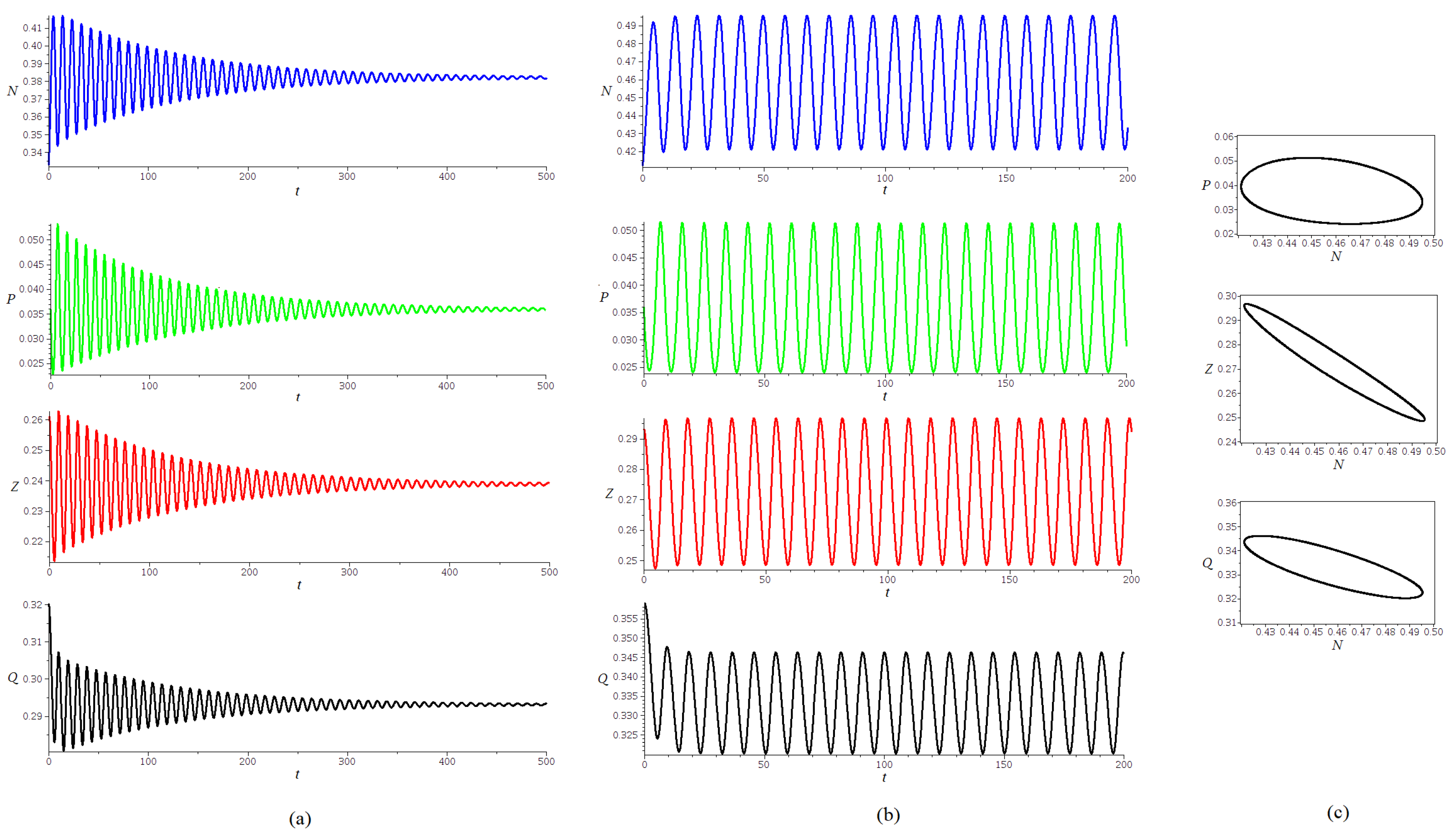
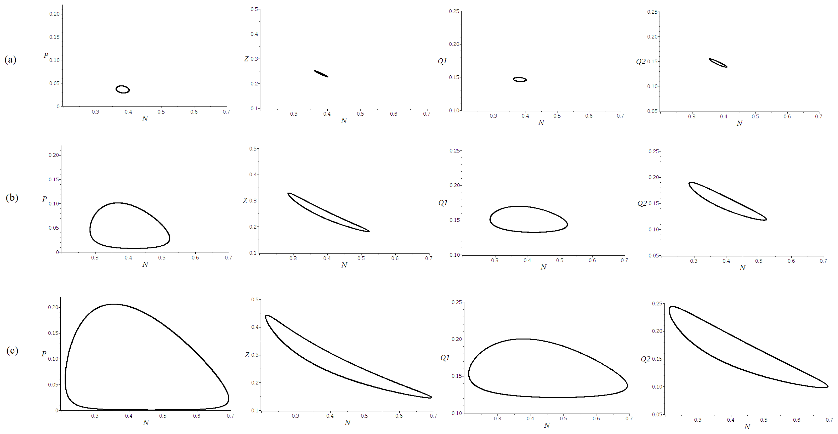
For
, the approximate value of
for the Hopf bifurcation is
. The simulations in
Figure 5, show the projections of parts of the trajectories for an initial point near the equilibrium
, proving an evolution towards a stable limit cycle, for (a)
, (b)
and (c)
.
The trajectories in
Figure 4 and
Figure 5 were obtained using the DEtools package in MAPLE 18, applying the fourth-order Runge–Kutta method, with a stepsize 0.01.
Remark 4. As the parameters vary away from the Hopf bifurcation curve, the limit cycle born through the Hopf bifurcation may disappear, may double the period, etc. Since the dimensions of both the weak and the strong models are greater than three, strange attractors may also exist. Nevertheless, as the domains for each of the two models are bounded, the ω-limit set for each model is also bounded, and so are their attractors.
6. Discussion
In this study, we have analysed two NPZ models for a closed ecosystem with three compartments, dissolved nutrient, phytoplankton and zooplankton, incorporating a delay in nutrient recycling. The models were obtained starting from a NPZ model introduced in [
12], by using the gamma distribution function with one or two degrees of freedom. The aim of the paper was to study how the stability and bifurcation of the equilibrium solutions depend on the total amount of nutrient and the delay.
We have shown that each of the two models have at most three equilibrium points in the region of interest, and that at most one of the equilibrium points is locally asymptotically stable at each value of the total nutrients. More precisely,
- (1)
For there is only one equilibrium point with no phytoplankton and no zooplankton (, which is asymptotically stable;
- (2)
For the equilibrium with phytoplankton and no zooplankton is asymptotically stable, while is unstable;
- (3)
As the first two equilibria are unstable, while the equilibrium with both phytoplankton and zooplankton is asymptotically stable either for all or there exists an such that is stable for , and unstable for close to depending on the response function
Further, we have proven that the changes of stability at and occur through transcritical bifurcations. Finally, we have shown that the change of stability at is a Hopf singularity and the associated bifurcation will lead to stable limit cycles if it is supercritical. Numerical simulations show the existence of stable limit cycles for each delay close to the bifurcation value
Thus, for each of the two considered models, the -limit sets contains at most one equilibrium point. In specific hypotheses on the response function h, the -limit sets may contain a limit cycle for certain values of the parameters and . However, as the dimension of both models is greater than 2, the -limit sets may also contain strange attractors.
Our results on the existence of equilibria are consistent with those of [
12] for the system with a general distribution (
1), who showed the equilibrium values of
are only affected by the mean delay and not the form of the distribution. The stability result (1) above reproduces that of [
12] for the general distribution case. The stability result (2) is stronger than that of [
12] for a general distribution, and thus is likely a consequence of our choice of distributions. In fact, [
12] showed that if the system has a discrete delay (Dirac distribution), then the equilibrium
may undergo a Hopf bifurcation; however, we show that it is not possible for the distributions we consider. Our results extend those of [
12] by proving the stability result (3) for the two systems studied and by proving the types of bifurcations that occur as the stability of the equilibrium points changes. Further, we showed the possibility of a codimension-two double Hopf bifurcation in the system with the two-degrees of freedom gamma distribution.
To conclude, we discuss the implications of our work for application. The general trend of bifurcations of the equilibrium points as the total amount of nutrients is increased is as follows: first, the phytoplankton only equilibrium point, , appears and then the coexistence equilibrium point, . This is is biologically plausible: as more nutrients are available, the system can support more organisms. Our work highlights the fact that a delay in the recycling can be stabilizing: the amount of nutrients needed for the transcritical bifurcation leading to the emergence of to occur increases with the size of the mean delay. We also showed, for a given amount of total nutrients, the delay decreases the equilibrium size of at least one of . This is because some of the nutrients are stored in the other compartments of the system, which represent the nutrients that are being recycled. Both these results were identical for the weak and strong models. Where these models differ was in the effect of the delay on the Hopf bifurcation of the equilibrium point. For both models, as the delay is increased we observe the same qualitative effect: the Hopf bifurcation value increases, then decreases, then increases. However, the variation is larger for the strong model than for the weak model. Thus, the for the weak model is less than that for the strong model for small enough delay, with the reverse for large enough delay.


